Optimal management strategies for a cascade reservoir system

(1)

UNIVERSITY OF SOUTHERN QUEENSLAND

OPTIMAL MANAGEMENT STRATEGIES FOR A

CASCADE RESERVOIR SYSTEM

Clayton Forknall B. Sc. with Distinction

Faculty of Health, Engineering and Sciences, The University of Southern Queensland

September 2014

(2)

(3)

c

by

(4)

CERTIFICATION OF DISSERTATION

I certify that the ideas, experimental work, results, analyses, software and conclusions reported in this dissertation are en-tirely my own effort, except where otherwise acknowledged. I also certify that the work is original and has not been previ-ously submitted for any other award, except where otherwise acknowledged.

Clayton Forknall Date

Endorsement

(5)

Abstract

Water reservoirs have long been used throughout Australia and the globe as a means of both providing communities with water security during periods of limited rainfall, as well as a form of defence against severe flooding. In recent times, the effective management of these water reservoirs has been questioned and is now, more than ever, under scrutiny.

In order to address the issue of reservoir mismanagement, this thesis demonstrates the methods and procedures undertaken in the development, formulation and ap-plication of two Mixed Integer Linear Programming (MILP) models that have the ability to determine strategies for the optimal management of a cascade reservoir system, under the two extreme environmental conditions of drought and flood. For the purposes of this thesis, the unique cascade configuration of a reservoir system was primarily considered; where cascade refers to a multiple reservoir system in which the spill from earlier reservoirs becomes a source of inflows to subsequent reservoirs. Many physical reservoir systems exhibit this type of layout including the Perseverance and Cressbrook system located near Toowoomba, which has been considered as a case study throughout this thesis.

By applying the drought and flood models to the case study of the Perseverance and Cressbrook cascade reservoir system, it was found that both models provided com-prehensive approximations of the system behaviours under the differing extreme conditions considered by each model. However, in order to conduct a successful comparison of the management strategies employed by the drought and flood mod-els, a common set of inflow records upon which both models could be considered was required. Rather than using a portion of the historic inflow records sourced for the case study considered, time series analysis was employed instead to select a time series model that suitably represented the historic records, and then from this model, an alternate set of inflows was simulated.

(6)

(7)

Acknowledgements

Throughout the creation and development of this thesis there have been many peo-ple (too many to mention here), who without their advice and support, this thesis would not be what it is today; I thank you!

First and foremost, I would like to thank Dr Trevor Langlands, who has provided sound, thoughtful guidance and excellent supervision from the genesis of this thesis through to its completion. His door was always open and I could not have hoped for a more knowledgeable, patient and supportive supervisor.

Many thanks also go to Dr Rachel King, for the effort and many hours of her time that she dedicated to proof reading this thesis. Her generous, helpful feedback and constructive comments proved invaluable. Along with her time, she also lent me her ear on many occasions; ensuring that I remained motivated, enthusiastic and sane (though that is debatable) over the course of this thesis.

Also, I would like to recognise the support and plentiful encouragement provided at just the right moments by Dr Christine McDonald, the knowledge, wisdom and experience shared by Associate Professor Ron Addie and the patience and under-standing offered by Associate Professor Richard Watson when life inevitably got in the way of study.

On top of this, I would like to thank Dr Alison Kelly and the team of biometricians (Susan, Kerry, Gaby and Dave) with whom I work, for their patience and the time needed to finish this thesis; they have been most accommodating and supportive throughout.

Last but definitely not least, I must thank my family and friends for the opportu-nity, time and exorbitant amount of encouragement and motivation (at times mixed with threats and ultimatums) that they provided in order to enable me to create this thesis.

(8)

(9)

3.3.2 Scenario 2: Initial Reservoir Capacities of 10 ML (S0 = 10), with 12 Months of Phase Two Rationing Permitted (n= 12) 47 3.3.3 Scenario 3: Initial Reservoir Capacities ofα2DML (S0 = α2D), with 6 Months of Phase Two Rationing Permitted (n = 6) . 51 3.3.4 Comparison of Releases to Community under Scenarios 1, 2 and 3. . . 55

4 Flood Model 61 4.1 Chapter Overview . . . 61

4.2 Models . . . 61

4.2.1 Model 5 - Flood Model adapted from that developed by Shih and ReVelle (1995) . . . 61

4.2.3 Model 6 - Extension of Flood Model . . . 70

4.3.1 Trial 1: Unconstrained Initial Capacities (S0 ≤C) . . . 81

4.3.2 Trial 2: Initial Capacities of 0 ML (S0 = 0) . . . 85

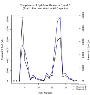
4.3.3 Trial 3: Initial Capacities of Half Reservoir Capacity (S0 = 1₂C) 89 4.3.4 Comparison of Spill from Reservoirs 1 and 2 under Trials 1, 2 and 3 . . . 92

5 Using Time Series to Simulate Inflows 99 5.1 Chapter Overview . . . 99

5.2 Selection of Time Series Model. . . 99

5.3 Diagnostic Tests . . . 106

5.4 Model Validation and Inflow Simulation . . . 112

6 Drought Model and Flood Model Comparison 119 6.1 Chapter Overview . . . 119

(11)

6.2.1 Exploration of the Behaviour of the Drought Model

Parameters . . . 123

6.2.2 Exploration of the Behaviour of the Flood Model Parameters 126 6.2.3 Comparison of Drought Model and Flood Model Management Strategies . . . 130

7 Conclusion 135 A Example of LINGO Input and Output - Model 2: The Simple Model 143 A.1 Example of LINGO Input for the Simple Model . . . 144

A.2 Example of LINGO Output for the Simple Model . . . 148

B Example of LINGO Input and Output - Model 4: The Drought Model 149 B.1 Example of LINGO Input for the Drought Model under Scenario 1 . 150 B.2 Example of LINGO Output for the Drought Model under Scenario 1 159 C Example of LINGO Input and Output - Model 6: The Flood Model 161 C.1 Example of LINGO Input for the Flood Model under Trial 1 . . . . 163

C.2 Example of LINGO Output for the Flood Model under Trial 1 . . . 172

D Tables of Inflow Records 173 D.1 Inflows under Worst Case Drought Scenario . . . 174

D.2 Inflows under Worst Case Flood Scenario . . . 175

D.3 Simulated Inflows from AR(1) Time Series Model . . . 176

D.4 Simulated Inflows to Reservoir 1 and Reservoir 2. . . 177

E Time Series Analysis Source Code 179 E.1 Formatting the Historic Data . . . 179

E.2 Fitting the Time Series Model . . . 180

E.3 Diagnostic Tests of Time Series Model . . . 182

E.4 Validation of Time Series Model . . . 184

E.5 Simulation of Inflows . . . 184

(12)

(13)

List of Tables

3.1 Comparison of the Releases to the Community from Reservoir 1 and

Reservoir 2, across the 3 Scenarios considered. . . 56

4.1 Summary Statistics of Volume Spilled under each Trial from

Reser-voir 1 and ReserReser-voir 2. . . 93

5.1 Comparison of the AIC for each Model Type fitted to the Historic

Inflow Traing Series. . . 105

D.1 Monthly Inflow to Cressbrook and Perseverance Dams under Worst

Case Drought Scenario from Historic Records . . . 174

D.2 Monthly Inflow to Perseverance and Cressbrook Dams under Worst

Case Flood Scenario from Historic Records . . . 175

D.3 Simulated Monthly Inflow from AR(1) Time Series Model. . . 176

D.4 Simulated Inflows to Reservoir 1 and Reservoir 2 from Time Series

(14)

(15)

List of Figures

1.1 Configuration of Cascade Reservoir System investigated as a Case

Study. . . 9

2.1 Policy 1: Resevoir Capacities (ML) against Community Water

Sup-ply Demand.. . . 18

2.2 Policy 1: Comparison of Resevoir Capacities. . . 19

2.3 Policy 2: Resevoir Capacities against Community Water Supply

De-mand. . . 21

2.5 Policy 3: Resevoir Capacities against Community Water Supply

De-mand. . . 23

3.1 Graphical Representation of the Relationship between Reservoir

Trig-ger Volumes and Rationing Levels. . . 29

3.2 Revised Graphical Representation of the Relationship between

Reser-voir Trigger Volumes and Rationing Levels.. . . 32

3.3 Monthly Inflow to Perseverance and Cressbrook Dams under Worst

Case Drought Scenario from Historic Records. . . 40

3.4 Scenario 1: Comparison of Reservoir Levels. . . 42

3.5 Scenario 1: Comparison of Releases to Community Water Supply. . 43

3.6 Scenario 1: Comparison of Reservoir Trigger Volumes.. . . 44

3.7 Scenario 1: Relationship between Available Water + Trigger Volumes

and Community Releases for Reservoir 1. . . 45

3.10 Scenario 2: Comparison of Releases to Community Water Supply. . 49

(16)

4.1 Simple Schematic of the Reservoir System considered in Model 5. . 64

4.2 Graphical Representation of the Relationship between Reservoir

Trig-ger Volumes and Pumping Restrictions. . . 65

4.3 Adapted Graphical Representation of the Relationship between

Reser-voir Trigger Volumes and Pumping Restrictions. . . 68

4.4 Simple Schematic of the Reservoir System considered in Model 6. . 73

4.5 Hourly Inflow to Perserverance and Cressbrook Dams under the

Worst Case Flood Scenario from Historic Records. . . 80

4.6 Trial 1: Comparison of Reservoir Levels. . . 82

4.7 Trial 1: Comparison of Spill from Reservoir 1 and Reservoir 2. . . . 83

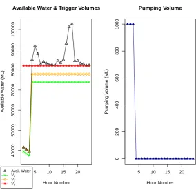
4.8 Trial 1: Relationship between Available Water + Trigger Volumes

and Pumping Volume for Reservoir 2. . . 84

4.10 Trial 2: Comparison of Spill from Reservoir 1 and Reservoir 2 . . . 87

4.13 Trial 3: Comparison of Spill from Reservoir 1 and Reservoir 2. . . . 90

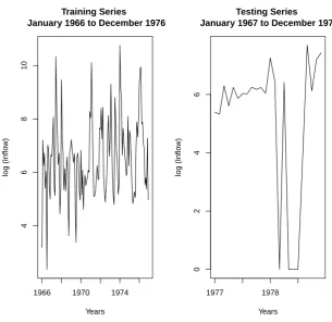
5.1 Logarithm Transformed Historic Inflows from Jan 1966 to Dec 1978. 100

5.2 Historic Inflows Separated into Training Series and Testing Series. . 101

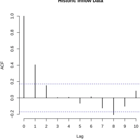
5.3 The Sample Autocorrelation Function (Sample ACF) for the Historic

Inflow Training Series. . . 102

5.4 The Sample Partial Autocorrelation Function (Sample PACF) for

the Historic Inflow Traning Series. . . 104

5.5 Example Output from the Time Series Model fitting process in R. . 105

5.6 Residual ACF and PACF for the AR(1) Model fitted to the Historic

5.7 Example of the Output from performing a Box-Pierce Test on the

residuals of the AR(1) Model in R. . . 108

5.8 Cumulative Periodogram of the Residuals for the AR(1) Model fitted

to the Historic Inflow Training Series. . . 109

5.9 Q-Q Plot of the Residuals for the AR(1) Model fitted to the Historic

(17)

5.10 Histogram of the Residuals for the AR(1) Model fitted to the Historic

5.11 Comparison of the Forecast Inflows from the AR(1) Model to the

Historic Inflows that compose the Testing Series.. . . 113

5.12 Resulting Output from the Simulation of Inflows performed using the

AR(1) Model in R. . . 114

5.13 Simulated Series of Inflows from the AR(1) Model found to provide

an approximate representation of the Historic Inflows. . . 115

6.1 Repeated Copy of Figure 1.1 showing the Configuration of the

Cas-cade Reservoir System investigated as a Case Study.. . . 120

6.2 Alternate Set of Inflows to Reservoir 1 and Reservoir 2 Simulated

using Time Series Analysis. . . 121

6.3 Drought Model: Behaviour of Reservoir 1 and Reservoir 2 Storage

Levels. . . 124

6.4 Drought Model: Behaviour of Available Water + Trigger Volumes

and the Relationship with the Community Releases for Reservoir 1. 125

6.5 Drought Model: Behaviour of Available Water + Trigger Volumes

and the Relationship with the Community Releases for Reservoir 2. 125

6.6 Flood Model: Behaviour of Reservoir 1 and Reservoir 2 Storage Levels.127

6.7 Flood Model: Behaviour of Spill from Reservoir 1 and Reservoir 2. . 128

6.8 Flood Model: Behaviour of Available Water + Trigger Volumes and

(18)

(19)

Chapter 1

Introduction and Literature Review

1.1

Introduction

The management and operation of a system responsible for the storage of a valuable commodity will always be a topic open for investigation and potential improvement, especially when the commodity is valuable enough to be referred to as“liquid gold”; water. Water reservoirs have long been employed around Australia and the globe to serve two main purposes; ensure communities have access to a reliable water supply during periods of limited rainfall or drought and to help protect communities from the impact of flood. This means that it is not only the operators of the reservoir sys-tems that are interested in their optimal management during these extreme events, but also the communities that rely upon the systems for one purpose or another. Therefore, this thesis aims to formulate and develop two mathematical models that can be employed to determine strategies for the optimal management of a cascade reservoir system under the two opposing extreme environmental conditions of a drought and flood. In this case, cascade refers to the unique layout of the reservoirs in the system, where releases from the spillway (termed spill) of a previous reservoir in the system become a source of inflows to subsequent reservoirs; thus influencing the volume of water, or storage level, of those subsequent reservoirs. Figure 1.1, provided at the end of this chapter, gives an example of the layout exhibited by a physical cascade reservoir system and how spill from one reservoir influences the storage level of the next.

(20)

Programming models. Although comprehensive, one shortcoming of this review by

Yeh(1985) was that it only considered models for the day to day management of a reservoir system and did not investigate models capable of describing the operation of a reservoir system during extreme environmental conditions, such as a drought or flood. Sometime later, a second state-of-the-art review was released by Labadie

(2004) investigating the optimal operation of multi-reservoir systems. In the work,

Labadie(2004) praises Linear Programming (LP) models as being one of the most

favoured optimisation techniques due to their efficiency and ability to converge to a global optimal solution. However, he goes on to discount Mixed Integer Linear Programming (MILP) models, an extension of Linear Programming and the pre-dominant modelling technique employed in this thesis, as being less computationally efficient than pure LP models (Labadie,2004). Although perhaps less computation-ally efficient, Mixed Integer Linear Programming provides an alternate method for representing constraints that would otherwise be nonlinear and, if included, severely increase the complexity of the model; a concession also made by Labadie (2004). Upon comparison to the review performed byYeh (1985), the more recent work by

Labadie(2004) investigated the use of computer based techniques such as heuristic

methods alongside simulation and neural network models; an indication of the ad-vances made in computer technology since the initial review performed in 1985. In a research area as broad as that of environmental management, under which the operation of a reservoir system falls, there are always situations and circumstances that are yet to be explored. Some of these situations were outlined by ReVelle

(2000), who provided an insight into the research challenges in environmental man-agement and defined some problems that, at the time, remained unsolved. An example of some of the topics explored by ReVelle (2000) included techniques for the management of parallel reservoirs, water quality, and solid wastes. In the in-vestigation of management techniques for parallel reservoirs, a basic LP model was provided as an example. This model is slightly more complex than the simple model formulated by ReVelle and McGarity (1997) that formed a foundation for research and experimentation in this thesis (explored thoroughly in Chapter 2). ReVelle

(21)

byChenet al.(2013) to manage the reservoir system were significantly different to those methods explored in this thesis, as they introduced the idea of a Flood Limit-ing Water Level as a parameter for assessLimit-ing the tradeoffs between flood control and conservation (Chenet al.,2013). Although the management strategies employed by

Chen et al. (2013) are fundamentally different to those proposed in this thesis for

the operation of a reservoir system in the event of a flood, the aim of both works are the same; to optimally manage a cascade reservoir system during a flood event.

1.2

Simple Model

Every thesis has a point of origin. In this case, that starting point was a simple LP model formulated by ReVelle and McGarity (1997) to describe the operation of a reservoir. The objective of the proposed model was to determine, given a known set of inflows, the minimum capacity of a reservoir required in order to ensure that a constant water demand could be confidently supplied to a community each month. This model was quite limited in its physical application; however it did provide a foundation for further research and experimentation, along with an appreciation of how such models behave and function. One suggestion thatReVelle and McGarity

(1997) offered when discussing multi-reservoir systems was that, if the reservoirs are arranged in a cascade configuration, then to avoid over complicating the problem the system should be treated as a single large reservoir. The work conducted as part of this thesis suggests otherwise, and that such an assumption would be a vast over simplification, resulting in many crucial and subtle details being omitted or overlooked. For example, if the system is assumed to be one large reservoir, the model would lack the ability to monitor the amount of spill from one reservoir to the next; an important detail that influences the selection of an optimal of management strategy for the system.

1.3

Drought Model

Droughts are an environmental phenomenon that occurs worldwide, where regions experience below average rainfall for an extended period of time. These events place increased stress on the water resources of the regions affected, especially when a country like Australia is considered. Renowned as one of the driest continents and continuously battling water shortage issues, Australia faces devastating conse-quences from drought. To make matters worse, under predicted climate change the duration and severity of these drought events are expected to increase (Easterling

et al., 2000), making it of the utmost importance that reliable and accurate

strate-gies exist to better manage water resources going into the future.

(22)

in order to find strategies that can be employed to better manage a reservoir system during a drought event. From the plethora of mathematical techniques presented by the research, one method suggested by the authors Shih and ReVelle (1995) formed the foundation of the work performed in this thesis. In their work,Shih and

ReVelle(1995) used a discrete hedging rule to formulate a MILP model to describe

the operation of a single reservoir during a drought event. This method followed on from previous work conducted by the same authors, in which they investigated the use of a continuous linear hedging rule for a single water reservoir (Shih and

ReVelle, 1994). After obtaining the optimal rule, the authors converted the

con-tinuous hedging rule into multiple discrete hedging rules, a form more suitable for practical applications, which then featured in their 1995 work. The work by Shih

and ReVelle (1995) is the only work found of this kind that formulates a MILP

model to explore the impact of a drought event on a reservoir used solely for water supply. Many other works focused on alternate aspects of the reservoir system, such as maintaining hydroelectric output during drought (ReVelle,2000), which are not applicable for the scenario investigated as part of this thesis.

An example of such a work is provided by the authorsTuet al.(2003) who developed a MILP model that considers both rule curves and hedging rules to optimize the operation of a multipurpose, multi-reservoir system. This reservoir system was not considered in isolation byTuet al.(2003), but instead was assumed to be connected to a large scale water distribution network, making the system far more complex than that explored in this thesis. Although there are significant differences in the size and complexity of the system considered, along with some of the methods used

by Tu et al. (2003), there are also similarities to the methods used in this thesis.

For example,Tuet al.(2003) differ from this thesis by employing network diagrams and initially formulating the problem using the minimum cost method; howeverTu

et al. (2003) did develop a MILP model to optimise the operation of the reservoir

system, a similar method to that employed in this thesis. The work by Tu et al.

(2003) could also become applicable if further research was to be conducted into the reservoir system considered in this thesis, this time incorporating the entire water distribution network of the region into the model.

(23)

were not as complex as that investigated by Tu et al. (2008). However, if more complex operating procedures were adopted by the managers of the reservoir sys-tem investigated as part of this thesis, the method implemented byTuet al. (2008) may provide a better approximation for the behaviours exhibited by components of the system.

As mentioned previously, many different methods exist to model the operation of a water reservoir system during a drought event. One such method is described by

Shiau(2003) who suggests the use of hedging rules in combination with a measure,

known as the reservoir supply index, to minimise the effects of drought on water reservoir systems. This reservoir supply index was developed to determine the onset and termination of water rationing and is defined as the probability of an available reservoir water supply being sufficient to meet an established demand (Shiau,2003). Effectively, the reservoir supply index is a probabilistic measure that evaluates the probability of a reservoir having sufficient water supplies to meet some predefined demand. In comparison to the work performed in this thesis, where the extent of water rationing is determined by the level of the reservoir itself, Shiau (2003) sug-gests the use of probabilities to predict the level of the reservoir into the future and thus the amount of rationing required. Although the method proposed by Shiau

(2003) may provide some lead time as to when it is best to enforce rationing, the probabilities could be misleading and either see rationing imposed when it is not needed or in contrast, see no rationing imposed when it is needed. By using the level of the reservoir itself to determine when rationing is enforced, and under the assumption that the demand from the reservoir, along with the inflows to the reser-voir are known, the occurrence of these types of errors have been minimised in this thesis.

Another method for modelling a water reservoir system during periods of water stress was suggested by the authors Srivastava and Awchi (2009). In their work, the authors used system analysis to develop a strategy that improved the perfor-mance of a reservoir system when the scenario of overstressed water utilisation conditions and demands was considered (Srivastava and Awchi, 2009). The tech-nique of system analysis incorporates a series of optimisation tools including Linear Programming, Dynamic Programming, Simulation, Artificial Neural Networks and hedging rules to determine an optimal management strategy for a reservoir system. In this case, the hedging rules that appeared in the system analysis conducted by

Srivastava and Awchi (2009) were based upon the series of discrete hedging rules

(24)

and ReVelle (1995) and adapting their work to function under a different set of circumstances was replicated in this thesis when developing both the drought and flood MILP models.

1.4

Flood Model

Floods are also an environmental phenomenon that occurs worldwide, where peri-ods of above average or extreme rainfall results in rivers and streams rising to a point where the flows can no longer be contained and the excess water inundates the surrounding regions. These events can prove deadly and often cause massive amounts of damage to the regions affected; impacting natural ecosystems and com-munities alike. Water reservoirs can be used as a form of defence against the worst impacts of a flood, as they provide a means of stalling the progression of floodwa-ters. Some reservoirs are designed with flood mitigation features, such as a gated spillway, which enables the progress of a flood to be halted and the floodwaters stored until the worst of the flooding event has passed, at which time releases from the reservoir can begin. As with droughts, the severity of floods is expected to increase under projected climate change (Easterling et al.,2000). Therefore, it is of vital importance that dependable strategies exist for the management of reservoir systems during a flood moving into the future.

(25)

of all the reservoirs in the system, where continuous spills from each reservoir oc-curred causing long periods of gradual changes in the storage levels. Both methods proposed had limited applicability to the system investigated in this thesis; however may prove useful if a larger cascade system was to be considered in future work. In more recent times, reservoirs have been constructed or upgraded to include flood mitigation measures such as gated spillways. These measures enable spill to be with-held until the river levels downstream of the reservoir have returned to a suitable level. Along with increasing the capabilities of reservoirs from water storage devices to flood defence mechanisms, these flood mitigation measures have also increased the scope of research that could be conducted in the area. An example of such research that has been performed into the operation of a reservoir featuring flood mitigation measures during a flood event is provided byKearneyet al.(2011). This work compared the existing mitigation strategy of Wivenhoe Dam in the Brisbane Valley, which features a gated spillway, to a model designed byKearneyet al.(2011) using the 2011 flood event in Queensland, Australia as a case study. Kearneyet al.

(2011) employed the method of model predictive control to develop a flood mitiga-tion strategy for the reservoir and then performed a simulamitiga-tion study to compare the outcome of their model to the already existing mitigation strategy for Wiven-hoe Dam. The method of model predictive control is significantly different to that utilised in this thesis, where the discrete hedging rules and MILP model proposed

byShih and ReVelle (1995) were adapted and altered to ensure their applicability

to a flood event.

(26)

when the operation strategies outlined in the Manual were employed, along with the measured inflows into the two reservoirs over the course of the event. These inflows were originally going to be used as a form of proxy data for the reservoir system considered in this thesis; however more suitable historic inflows were able to be sourced from the Queensland Department of Natural Resources and Mines

(2012).

1.5

Time Series Analysis

Although historic inflows were able to be sourced for the cascade reservoir system considered as part of this thesis, time series analysis was utilised to generate another dataset based on the historic records. In order to formulate a time series model for the data, the methods introduced by Dunn and Addie (2008) were employed. In their work, they presented two selection tools that could be used to determine a suit-able time series model to describe a given dataset. Once a model was selected,Dunn

and Addie (2008) outlined a battery of diagnostic tests that could be performed in

order to ensure that the model selected provided an approximate representation of the historic inflow records by capturing the important information, or signal, of the data. Dunn and Addie(2008) also outlined a method for generating a series of one-step ahead forecasts from the time series model to test its accuracy when com-pared to a portion of the original dataset. Each of these methods was performed in this thesis and resulted in the development of a time series model that adequately described the historic inflow records. This model was then employed to generate another series of data which could be used as a common set of inflows when per-forming a comparison of the management strategies employed by the drought and flood models.

1.6

Case Study: Perseverance and Cressbrook Dams

The extent of this thesis is not limited to the development of MILP models, but also includes the application of these models to an existing cascade reservoir sys-tem in order to determine optimal strategies for the management of such a syssys-tem during a drought and flood event. In this case, two of the reservoirs that contribute to the water supply of the Toowoomba region exhibit a cascade configuration; be-ing the Perseverance and Cressbrook dams. Both of these reservoirs are located approximately 35 kilometres northeast of Toowoomba and make up two thirds of the regions reservoir system, with another solitary dam located to the north of Toowoomba also contributing to the water supply network (Toowoomba Regional

Council, 2013). Figure 1.1 displays the geographical layout of the Perseverance

(27)

[image:27.595.135.516.82.373.2]

Figure 1.1: Configuration of Perseverance and Cressbrook cascade reservoir system investigated as a Case Study.

Black Rectangles = Dam Spillway, Thinner Blue Arrows = Sources of Inflows,

Thicker Red Arrows = Direction of Spill from Perseverance to Cressbrook dam.

seen that Cressbrook dam is the larger of the two reservoirs, with an approximate maximum available storage of 82 000 megalitres (ML), whilst Perseverance dam is smaller with approximately 30 000 ML of maximum available storage (Toowoomba

Regional Council, 2013). As stated previously, when in a cascade configuration,

(28)

(29)

Chapter 2

Simple Model

2.1

Chapter Overview

The focus of this chapter is to demonstrate where this thesis began; with the explo-ration and extension of a simple model used to describe the opeexplo-ration of a reservoir system. To begin, the simple Linear Programming (LP) model presented by

ReV-elle and McGarity (1997) is stated and investigated. Labelled Model 1, this model

was rather limited in its applicability to a physical system and therefore required extension in order for it to adequately describe the operation of a cascade reservoir system. The extended form of the simple model, named Model 2, can also be found in this chapter along with a review of the results from an experiment conducted using the model. Although both Model 1 and Model 2 are simplistic and not as comprehensive as other models explored later in this thesis, the work conducted in this chapter formed a basis of understanding regarding how LP models can be applied to describe the operation of a reservoir system.

2.2

Models

2.2.1 Model 1 - Simple Model developed by ReVelle and McGarity (1997)

In this section, the first of two models explored in this chapter is introduced. For-mulated by ReVelle and McGarity (1997) to describe the fundamental behaviours exhibited by a single reservoir system, Model 1 is given below in Equations (2.1) to (2.5). Note that a description of the constraints and variables used to compose the simple LP model are provided in Section 2.2.2:

minimise z =c (2.1)

such that

St=St−1+It−q−Wt ∀t, (2.2)

St≤c ∀t, (2.3)

ST ≥S0, (2.4)

(30)

2.2.2 Model 1 Description

Model 1 is a straightforward LP model that measures the storage level of a single reservoir system over a time period of known length. The authors of Model 1 state that the objective of this model is to determine the smallest reservoir capacity required to sustain a steady release from the reservoir for use as a water supply over the duration of the time period specified; while, at the same time ensuring that the ending reservoir condition is no worse than the condition of the system at the beginning of the time period (ReVelle and McGarity,1997).

Variable Definitions

There are eight variables that are used in the formulation of Model 1. These vari-ables can be defined below:

t, T = the index and the total length of the time period considered, in this case assumed to be months,

St = the storage level of the reservoir at the end of montht, which is unknown

(megalitres, ML),

S0 = the unknown initial storage level of the reservoir (ML),

q = the specified steady month-to-month release from the reservoir for use as a water supply (ML),

Wt = the unknown amount of spill from the reservoir in month t (ML), c = the unknown reservoir storage capacity (ML),

It = the historical inflows to the reservoir in month t, which are specified

(ML).

In order to investigate how these variables feature and interact in Model 1, the constraints that compose the model can be investigated.

Contraint Definitions

(31)

Equation (2.5) is included to ensure that particular variables remain nonnegative and thus physically realistic.

2.2.3 Model 2 - Extension of Simple Model

Upon experimentation of Model 1, it was found that the model had limited applica-bility to a physical system and required extension in order to suitably describe the operation of a cascade reservoir system. This extended model, labelled Model 2, is given below in Equations (2.6) to (2.28). Note that variables labelled with a star (*) correspond to Reservoir 1, whilst variables without a star relate to Reservoir 2.

minimise z =C_D∗ +CD (2.6)

such that

Reservoir 1 Constraints

S_t∗ =S_t−1∗ +I_t∗ −q∗−W_t∗ ∀t, (2.7)

S₀∗ ≤C_D∗, (2.8)

S_t∗ ≤C_D∗ ∀t, (2.9)

W_t∗ ≤C_S∗ ∀t, (2.10)

C∗ =C_S∗ +C_D∗, (2.11)

C_S∗ ≤0.1C_D∗, (2.12)

St−1∗ +It∗−q ∗₋

C_D∗ =p+_t ∗−p−_t ∗ ∀t, (2.13)

p−_t∗ ≤M y∗_t ∀t, (2.14)

p+_t∗ ≤M(1−y_t∗) ∀t, (2.15)

W_t∗ ≤p+_t∗ ∀t, (2.16)

(32)

Reservoir 2 Constraints

St=St−1+It−q−Wt+Wt∗ ∀t, (2.18)

S0 ≤CD, (2.19)

St≤CD ∀t, (2.20)

Wt ≤CS ∀t, (2.21)

C =CS+CD, (2.22)

CS ≤0.1CD, (2.23)

St−1+It−q−CD =p+t −p −

t ∀t, (2.24)

p−_t ≤M yt ∀t, (2.25)

p+_t ≤M(1−yt) ∀t, (2.26)

Wt ≤p+t ∀t, (2.27)

St, St−1, It, Wt, p+t, p −

t ≥0 ∀t. (2.28)

Model 2 builds upon the framework provided by Model 1 to formulate a model that is capable of describing the basic behaviour exhibited by components of a cascade reservoir system. In this sense, the model measures the storage levels of two reservoirs situated in a cascade configuration over a time period of known length. The objective function of Model 2 also builds upon that stated for Model 1; determining the smallest reservoir capacities required to sustain a steady release to a water supply, where the water supply is shared between the two reservoirs, over the duration of the time period considered.

(33)

There are 14 variables used in the formulation of Model 2. Seven of these variables were defined previously when describing Model 1 in Section2.2.2, under the heading Variable Definitions. The seven remaining variables that have not been defined previously are listed below:

C = the total reservoir capacity, which is unknown (ML),

CD = the unknown reservoir storage capacity (ML),

CS = the unknown capacity of the reservoir spillway (ML),

p+_t = an indicator variable whose value is greater than zero if spill is occurring from the reservoir in month t, which is unknown (ML),

p−_t = an indicator variable whose value is greater than zero if no spill is occur-ring from the reservoir in month t, which is unknown (ML),

M = a large constant value, assumed to equal 10 000 in this case,

yt = an unknown binary variable that equals 0 if spill is occurring in month t

or 1 otherwise.

How these variables feature and interact can be explored through the investigation of the constraints that compose Model 2.

Constraint Definitions

Model 2 consists of an objective function and 22 constraints, eleven of which are repeated from Reservoir 1 to Reservoir 2. In this case, as Model 2 is applicable to a dual cascade reservoir system, the objective function (Equation (2.6)) contains both variables C_D∗ and CD and aims to minimise the storage capacities of the two

reservoirs subject to the other constraints in the model. Equations (2.7) and (2.9) have been defined previously in Section 2.2.2 for Model 1; the first is the mass balance constraint, whilst the second ensures that the reservoir storage level does not exceed the reservoir storage capacity in any given month. Equation (2.8) ensures that the initial reservoir storage level does not exceed the reservoir storage capacity, while Equation (2.10) makes certain that the amount of spill in a month does not exceed the spillway capacity. Equation (2.11) is an equality constraint stating that the total reservoir capacity is equal to the reservoir storage capacity plus the reservoir spillway capacity. Equation (2.12) is then included to limit the size of the spillway capacity to a proportion of the reservoir storage capacity, in this case arbitrarily selected to be 10%. Equation (2.13) is used to measure the extent of spill (if any) that occurs from a reservoir in a given month.

(34)

exit the reservoir as spill. If spill occurs, the extent of the spill is measured by the variablep+_t. On the other hand, if spill does not occur in the current month, then the extent by which the storage level is below the reservoir storage capacity is measured by the variable p−_t . These variables are used in conjunction with Equations (2.14) and (2.15) to determine the value of the binary variable yt. As stated earlier, the

value of the variable yt equals zero if spill is occurring in the current month or one

otherwise. This can be illustrated by an example; if spill is occurring in the current month, then the variable p+_t will have a value greater than zero, while the variable

p−_t has a value of zero. In order to satisfy both Equation (2.14) and (2.15), the variable yt must also have a value of zero. If the alternate situation is considered,

where no spill occurs in the current month, then the variable p+_t will have a value of zero, while the variablep−_t has a value greater than zero. Once again, in order to satisfy both constraints, the variable yt must have a value of one. Equation (2.16)

then states that the amount of spill that occurs in the current month must be at most equal to the variablep+_t. Equation (2.17) is included to ensure that particular variables remain physically realistic and thus nonnegative. At this point, it should be noted that Equations (2.19) to (2.28) are the same as Equations (2.8) to (2.17); however are applicable to Reservoir 2. The only constraint that varies between the two reservoirs is the mass balance constraint; Equations (2.7) and (2.18). In the case of Reservoir 2, it contains the additional variableW_t∗; the amount of spill from Reservoir 1 in the current month. As the two reservoirs are situated in a cascade configuration, spill from Reservoir 1 becomes a source of inflows to Reservoir 2 and as such needs to be included in the mass balance constraint of the second reservoir.

2.3

Results and Discussion

In this section, an experiment to investigate how the storage capacities of two reservoirs in a cascade configuration behave given varying community water supply requirements is conducted using Model 2. This experiment not only provided a means of applying and thus testing Model 2, but also offered a broader opportu-nity to better understand how simple LP and MILP models can be applied to the operation of reservoir systems.

In order to perform the experiment, the optimisation modelling software LINGO version 14.0 was employed (LINDO Systems Inc, 2013). An example of the syntax required to perform this experiment, along with an excerpt of the resulting output can be found in Appendix A.

(35)

month. Additionally, it was assumed that the releases from the reservoirs to the community water supply varied in 10 ML increments from a possible demand of 0 ML to 200 ML per month.

The final assumption made regarding the parameters of the experiment was to spec-ify that the two reservoirs shared the community water supply demand, according to a known policy. In order to explore how the reservoir capacities behaved under varying circumstances, three policies were invented; the first where the commu-nity water supply was split equally between the two reservoirs at 50% each, the second where Reservoir 1 was responsible for 70% of the community water supply and Reservoir 2 for the remaining 30%, and the final policy where Reservoir 1 was responsible for only 30% of the community water supply, while Reservoir 2 supplied 70%.

2.3.1 Policy 1

The first policy considered shared the community water supply demand equally be-tween the two reservoirs, at 50% each. In order to investigate how the capacities of the two reservoirs behaved under varying demand from the community, a series of plots have been constructed; Figure2.1demonstrates the behaviour of the reservoir capacities against community water supply separately, while Figure2.2displays the capacities of the two reservoirs on the same axis as a means of comparison.

From Figure 2.1 it can be seen that when there was no demand for water from the community, Model 2 predicted that a storage capacity of approximately 300 ML was required for both reservoirs. This result is contrary to first thought, which would suggest that if there is no demand by the community for water, then there is no need for a reservoir. However, the model assumed that the reservoir system was already in place and as such increased the reservoir capacity due to Equations (2.12) and (2.23). These constraints limit the capacity of the reservoir spillway to 10% of the reservoir storage capacity. Therefore, Model 2 elected to increase the storage capacity of the reservoir in order to maximise the capacity of the spillway and thus the amount of water that could be released from the reservoirs as spill each month.

(36)

● ● ● ● ● ● ● ● ● ● ● ● ● ● ● ● ● ● ● ● ●

0 50 100 150 200

0 50 100 150 200 250 300 Reservoir 1

Community Water Supply Demand (ML)

Reser

v

oir Stor

age Capacity (ML)

0 50 100 150 200

0 50 100 150 200 250 300 Reservoir 2

Reser

v

oir Stor

age Capacity (ML)

Reservoir Storage Capacities under varying Community Water Supply Demand (Constant Inflows = 50ML/month)

Figure 2.1: Policy 1 - Reservoir Capacities against Community Water Demand. Community Water Demand shared - Reservoir 1 at 50% and Reservoir 2 at 50%.

Left - Resevoir 1, Right - Reservoir 2.

50 ML per month and thus balancing the system. In context, this means that if it is known that 100 ML per month in total will be readily available from a river system, then the community could pump their requirements directly from the river without the need for a reservoir system. However, in practice, it is known that access to a steady water supply through rivers and streams cannot be assured and that some form of storage is necessary to ensure water security. In that sense, this component of the model is unrealistic; however this limitation is improved upon in subsequent chapters.

(37)

● ● ● ● ● ● ● ● ● ● ● ● ● ● ● ● ● ● ● ● ●

0 50 100 150 200

0 50 100 150 200 250 300

Comparison of Reservoir Storage Capacities (Constant Inflows = 50ML/month)

Reser

v

oir Stor

age Capacity (ML)

● _{Reservoir 1} Reservoir 2

Figure 2.2: Policy 1 - Comparison of Reservoir Capacities.

Community Water Demand shared - Reservoir 1 at 50% and Reservoir 2 at 50%.

needing to be supplied to the community in total. Under Policy 1, the demand from the community was sourced equally from the two reservoirs, resulting in the total increase of 60 ML being shared between the two reservoirs at 50% each; equating to an extra 30 ML needing to be stored in each reservoir to ensure that the community water supply demand could be met.

In addition to Figure 2.1, Figure 2.2 has been provided to compare the behaviour of the two reservoir capacities on a common set of axes. Evident from this figure is that the two reservoir capacities demonstrated much the same behaviour, except that the capacity of Reservoir 1 was slightly smaller than that of Reservoir 2 when the community water demand was less than 100 ML. This difference was attributed to the reservoirs being located in a cascade configuration, and any spill from Reser-voir 1 becoming a source of inflow to ReserReser-voir 2. Therefore, in order to combat the combined inflows to the second reservoir, the model elected to increase the storage capacity of Reservoir 2 and in doing so, the capacity of the reservoir spillway, in order to maximise the amount of spill from the reservoir when the inflows exceeded demand.

(38)

the minimum storage capacity of the reservoirs that at the same time maximised the size of the reservoir spillways, in order to release the unrequired, additional inflows. On the other hand, the second behaviour occurred when the inflows to the reservoir system were insufficient to meet the demand from the community each month. If this transpired, the reservoirs were required to store an additional volume of water in order to ensure that the community water demand could be maintained over the time period considered and, as such the capacities of the reservoirs increased proportional to this additional volume required. These two key behaviours of the reservoir storage capacities were also apparent in the other policies considered; how-ever were influenced by the unequal sharing of the community water demand and were more difficult to identify.

2.3.2 Policy 2

The next policy to be investigated shared the community water supply demand between Reservoir 1 and Reservoir 2 at 30% and 70% respectively. This sharing of community water demand could occur as a result of convenience or for cost reasons if one of the reservoirs was to be located closer to the community, or if one of the reservoirs was supplied by more substantial tributaries. Similar to Policy 1, two plots have been constructed to explore the capacities of the reservoirs against vary-ing community water supply demand and are given in Figure2.3 and Figure 2.4. From Figure 2.3, it can be seen that when there was no demand for water from the community, the model selected the same capacities for both reservoirs as those observed under Policy 1; approximately 300 ML. This behaviour is to be expected and witnessed again for the final policy, as the unequal sharing of community de-mand has no impact if there is no dede-mand to share (0 ML). As the dede-mand from the community increased, the capacity of both reservoirs decreased at constant rates until the community water demand reached approximately 80 ML per month. At this value, the community demand from Reservoir 2 began to exceed the inflows to the reservoir and as such, the behaviour of the reservoir capacity changed to reflect the need for water to be stored. On the other hand, the capacity of Reservoir 1 continued to decrease constantly until the critical demand volume of 100 ML per month was reached.

Upon the community water supply demand reaching 100 ML per month, Figure2.3

(39)

● ● ● ● ● ● ● ● ● ● ● ● ● ● ● ● ● ● ● ● ●

0 50 100 150 200

0 50 100 150 200 250 Reservoir 1

Reser

v

oir Stor

age Capacity (ML)

0 50 100 150 200

0 100 200 300 400 500 Reservoir 2

Reser

v

oir Stor

age Capacity (ML)

the community water demand, while the remaining 70% was sourced from Reservoir 2; translating to 30 ML and 70 ML per month being sourced from Reservoir 1 and Reservoir 2 respectively when the total community water supply demand per month equalled 100 ML. Therefore, by increasing the capacity of Reservoir 1 to 200 ML, Model 2 also increased the capacity of the Reservoir 1 spillway to 20 ML (the spill-way capacity is limited to 10% of the reservoir storage capacity by Equations (2.12) and (2.23)). This meant that the community demand of 30 ML per month from Reservoir 1 could be completely supplied out of the 50 ML of constant inflows to the reservoir each month, while the remaining 20 ML of inflows became spill from the reservoir. As the reservoirs were situated in a cascade configuration, the 20 ML of spill from Reservoir 1 combined with the constant inflow of 50 ML per month to Reservoir 2, thus providing a total inflow of 70 ML per month to the second reservoir. This combined inflow of 70 ML per month equated to the community demand of 70 ML per month from Reservoir 2; thus balancing the input and output of the reservoir and causing Model 2 to deem it unnecessary.

(40)

● ● ● ● ● ● ● ● ● ● ● ● ● ● ● ● ● ● ● ● ●

0 50 100 150 200

0 100 200 300 400 500

Comparison of Reservoir Storage Capacities (Constant Inflows = 50ML/month)

Reser

v

oir Stor

age Capacity (ML)

increase of 10 ML per month in community water demand. On the other hand, the capacity of Reservoir 2 increased at a constant rate of 60 ML for each 10 ML per month increase in the demand from the community.

(41)

● ● ● ● ● ● ● ● ● ● ● ● ● ● ● ● ● ● ● ● ●

0 50 100 150 200

0 100 200 300 400 500 Reservoir 1

Reser

v

oir Stor

age Capacity (ML)

0 50 100 150 200

0 50 100 150 200 250 300 Reservoir 2

Reser

v

oir Stor

age Capacity (ML)

2.3.3 Policy 3

The final policy to be investigated was when the community water supply demand was shared unequally between Reservoir 1 and Reservoir 2 at 70% and 30% respec-tively, or a reversal of that considered under Policy 2. As mentioned previously, this situation could occur when a more substantial river or stream system supplied one of the reservoirs, or if one reservoir was located closer to the community that the reservoir system was responsible for supplying. As before, two plots have been constructed to explore the behaviour of the reservoir capacities against varying com-munity water demands.

(42)

● ● ● ● ● ● ● ● ● ● ● ● ● ● ● ● ● ● ● ● ●

0 50 100 150 200

0 100 200 300 400 500

Comparison of Reservoir Storage Capacities (Constant Inflows = 50ML/month)

Reser

v

oir Stor

age Capacity (ML)

the storage of water in order to ensure the community demand could be maintained across the time period, occurred at a smaller community water supply demand than that seen under the previous policies. In this case, once the community water de-mand reached approximately 70 ML per month, the inflows to Reservoir 1 were no longer sufficient to supply the community alone and the reservoir needed to begin the storage of water. On the other hand, as 30% of the community water supply demand was sourced from Reservoir 2 under Policy 3, the transition in reservoir storage capacity behaviour occurred at a much larger value of community demand than seen previously; approximately 170 ML per month in this case.

(43)

2.4

Chapter Conclusion

This chapter has presented the work, models and material that formed the origin of this thesis. To begin, the simple LP model formulated by ReVelle and McGarity

(1997) was presented and described. This model was found to be limited in its ability to comprehensively describe the behaviours of a physical reservoir system and therefore required extension in order to be applicable to a cascade reservoir system. The extended model, named Model 2, was stated and a full description of the variables and constraints that compose the model provided. Following this, the results of an experiment to investigate how the capacities of two reservoirs in a cascade reservoir system behave under varying community water supply demands were provided. The experiment was replicated for three different policy types that specified how the community water demand was shared between the two reservoirs. From this experiment, it was found that the reservoir capacities behaved in two distinct ways; one when the inflows to the reservoir exceeded the demand from the community and the other when the inflows were insufficient to solely meet the community demand. Also, it was noted that Model 2 had some limitations and did not always provide informative results; in some cases suggesting that either one or both of the reservoirs in the system were not needed. In future chapters, some of these limitations are resolved.

(44)

(45)

Chapter 3

Drought Model

3.1

Chapter Overview

Extended periods of below average rainfall, known as drought, can place extreme stress on the water resources of regions affected. Therefore, optimal management strategies for reservoir systems, like those investigated in this chapter, are vital to ensure that communities have access to a reliable water supply throughout the extent of such an event.

To begin this chapter, a model proposed byShih and ReVelle(1995), labelled Model 3, for the operation of a single reservoir system during drought is explored. This Mixed Integer Linear Programming (MILP) model forms the foundation not only for work performed in this chapter, but for work conducted in Chapter 4 as well. Although very informative, Model 3 is only applicable to a single reservoir system and therefore required extension in order for it to be effective in investigating the cascade reservoir system considered as a case study in this thesis. This extended form of the drought model, denoted as Model 4, is also thoroughly investigated in this chapter, with each of the constraints and variables that compose the model being identified and defined. An experiment is then conducted in order to ascertain how components of the cascade reservoir system measured by Model 4 behave under varying drought conditions. These results form the basis of a discussion and a series of conclusions are made regarding the applicability of the extended model to the case study considered of an existing cascade reservoir system.

3.2

Models

3.2.1 Model 3 - Drought Model developed by Shih and ReVelle (1995)

In this section, the Mixed Integer Linear Programming (MILP) model formulated

byShih and ReVelle (1995) for the operation of a single reservoir during a drought

(46)

the constraints and variables used to formulate the model are provided in Section

3.2.2.

maximisez =

T

X

t=1

y1t−ω 12

X

p=1

(V1p+V2p+V3p) (3.1)

such that

y1t≥

(St−1+ ˆIt)−(V1p−)

M ∀t, p, (3.2)

y1t≤1−

V1p−(St−1+ ˆIt)

M ∀t, p, (3.3)

y2t≥

(St−1+ ˆIt)−(V2p−)

M ∀t, p, (3.4)

y2t≤1−

V2p−(St−1+ ˆIt)

M ∀t, p, (3.5)

Rt= (1−α1).D.y1t+ (α1−α2).D.y2t+α2.D ∀t, (3.6)

St=St−1+It−Rt−Wt ∀t, (3.7)

St≤C ∀t, (3.8)

S0 ≤ST, (3.9)

Ut≤ St

C ∀t, (3.10)

Wt ≤M Ut ∀t, (3.11)

V1p ≥(1 +β1)V2p ∀p, (3.12)

V2p ≥(1 +β2)V3p ∀p, (3.13)

V3p ≥α2.D ∀p, (3.14)

St−1+ ˆIt ≥V3p+ ∀t, p, (3.15)

y1t−1+y1t+1 ≤1 +y1t ∀t, (3.16)

y1t≤y2t+1 ∀t, (3.17)

T

X

t=1

y2t=T −n ∀t, (3.18)

St, St−1,Iˆt, It, V1p, V2p, V3p, Rt, Wt≥0 ∀t, p. (3.19)

As can be seen from the statement of Model 3 above,Shih and ReVelle(1995) have formulated a model substantially more complex than Model 1 and 2 investigated in the previous chapter.

(47)

Storage Plus Projected Inflow Releases to

Community Water Supply

0

Infeasible

Full Demand Released

Phase One Rationing

Phase Two Rationing

(𝑆𝑡−1+ 𝐼 𝑡)

𝑉3𝑝 𝑉2𝑝 𝑉1𝑝

(𝑅_𝑡)

𝐷

𝛼₁𝐷

𝛼₂𝐷

Figure 3.1: Graphical Representation of the Relationship between Reservoir Trigger Volumes and Rationing Levels.

Adapted from that presented by Shih and ReVelle (1995); where,

V1t, V2t, V3t = Trigger Volumes, D = Total Community Demand,

α1, α2 = Restrictions on the Releases to the Community.

the technique of rationing levels. In the case of Model 3 it has been assumed that there are three rationing levels; no rationing, phase one rationing and phase two rationing. For these levels to be put into effect, the model seeks to identify three trigger volumes, V1p, V2p, and V3p, for all months p. The values of these trigger

volumes are optimally derived by the model, except for the lower boundary trigger volume,V3p, which is determined through the specification of other variables by the

operators of the reservoir system. The relationship between the trigger volumes and rationing levels is summarised by Shih and ReVelle (1995) as follows:

“If the storage at the end of the previous period plus projected inflows are together greater thanV1p, then no water restrictions are announced.

If the storage at the close of the previous period plus projected inflows fall between V1p and V2p, then rationing phase one is assumed to be

declared, reducing demand to α1 proportion of its expected value. If

the storage plus projected inflow fall belowV2p, rationing phase two will

be declared and only the proportionα2of usual demand will be expected

to occur.” (Shih and ReVelle, 1995)

Figure 3.1 above provides a graphical representation of the relationship between the trigger volumes and the rationing levels of the reservoir. Also depicted by the figure is the assumption that if the storage plus projected inflow decreases below the lowest trigger volume of V3p, the outcome of the model is infeasible. For this

(48)

unrealistic and has therefore been relaxed in the development of Model 4 later in this chapter.

In order to enforce the technique of rationing, the objective of Model 3 is twofold. The first component of the objective function (Equation (3.1)) aims to maximise the number of months in which no rationing is enforced on the community water supply, meaning that the full demand is able to be released. In conjunction with this, the second component of the objective function attempts to minimise the trigger volumes across all monthsp. By minimising the trigger volumes, the length of time before rationing is imposed can be maximised. By incorporating these two components in the objective function, the number of months in which rationing is enforced is minimised, and as such the releases to the community are maximised.

There are 24 variables that compose Model 3. These variables are defined below:

t, T = the current month and the total number of months in the event horizon which are known,

p = p∈ {1,2, ...,12}, the month number of the year being considered. If the event horizon encompasses more than one year, this variable provides an index of the month number in the current year;

y1t = an unknown binary variable that is 1 if no rationing is applied in month t or 0 otherwise;

y2t = an unknown binary variable that is 1 if the system is at phase one

ra-tioning or better in month t, or 0 otherwise,

ω = a small number, which is assumed to equal 0.01 in this case,

V1p = the unknown value of storage and inflow above which no restrictions on

water use are placed (megalitres, ML),

V2p = the unknown value of storage and inflow below which phase two rationing

is implemented for month p(ML),

V3p = the specified lower bound of storage plus inflow for month p (ML), St = the storage in the reservoir at the end of month t, which is unknown

(ML),

It = the inflow to the reservoir in month t, which is known (ML),

ˆ

It = the projected inflow to the reservoir in month t, which is known (ML), = a small number, which is assumed to equal 0.1 in this case,

M = a big number, which is assumed to equal 100 000 in this case,

Rt = the releases to community water supply in month t, which is unknown

(49)

α1 = the specified percentage of total demand released to the community under

phase one rationing,

α2 = the specified percentage of total demand released to the community under

phase two rationing,

D = the specified total demand required by the community, which is assumed constant over the event horizon (ML),

Wt = the spill from the reservoir in month t, which is unknown (ML), C = the capacity of the reservoir, which is known (ML),

Ut = an unknown binary variable that is 1 if the reservoir is at full capacity

at the end of month t, or 0 otherwise,

β1 = a specified separation value, assumed throughout the chapter to be 0.05, β2 = a specified separation value, assumed throughout the chapter to be 0.05, n = the specified number of months in which it is deemed that phase two

rationing is acceptable.

The way in which these variables interact and behave can be investigated through the exploration of the constraints featured in Model 3.

Contraint Definitions

Model 3 consists of 18 constraints, plus the objective function. As mentioned pre-viously, the objective function (Equation (3.1)) is composed of two terms. The first and primary term of the function is to maximise the number of months in which no rationing is required. The secondary term then aims to minimise the total of the trigger volumes. By minimising the trigger volumes, the frequency at which rationing will be put into effect will be minimised. A weight is also placed on the trigger volumes to reduce the impact of this secondary term on the primary term of the function.

Equation (3.2) and (3.3) work together to calculate the value of the binary variable

y1t. If in the case of Equation (3.2), the reservoir storage level at the end of the

previous month plus the projected inflow this month, herein referred to as available water, is greater than the trigger volumeV1p, theny1twill equal one; indicating that

no rationing is required in the current month. On the other hand, Equation (3.3) requires that y1t equal zero if the available water is less than V1p; meaning some

amount of rationing is required. Shih and ReVelle (1995) explain that if the small value of was not included in these constraints, then when the available water equals the trigger volume (St−1 + ˆIt =V1p) the value of y1t could be either zero or

one. To correct this, is included in the constraint to ensure that y1t must equal

one if this was to occur.

(50)

Available Water (Storage Plus Projected Inflow) Releases to

Community Water Supply

0

Infeasible

Full Demand Released

Phase One Rationing

Phase Two Rationing

𝑉3𝑝 𝑉2𝑝 𝑉1𝑝

(𝑅_𝑡)

𝐷

𝛼₁𝐷

𝛼₂𝐷

𝒚_𝟏𝒕= 𝒚_𝟐𝒕= 𝟏 𝒚_𝟏𝒕= 𝟎

𝒚_𝟐𝒕= 𝟏

𝒚𝟏𝒕= 𝟎

𝒚𝟐𝒕= 𝟎

Figure 3.2: Revised Graphical Representation of the Relationship between Reservoir Trigger Volumes and Rationing Levels, showing the Values of the Binary Variables

y1t and y2t under each Level.

Adapted from that presented by Shih and ReVelle (1995); where,

V1t, V2t, V3t = Trigger Volumes, D = Total Community Demand,

α1, α2 = Restrictions on the Releases to the Community.

equal one if the available water is greater than the trigger volumeV2p. By equating

the value ofy2tto one, this indicates that phase one rationing will be required in the

current month. However, if the available water is less thanV2p, then Equation (3.5)

ensures thaty2t is equal to zero, leading to phase two rationing being implemented

in the current month. Shih and ReVelle (1995) point out that the four constraints, Equations (3.2) to (3.5), also assure thaty1t will not equal one unlessy2t equals one

and that if y2t equals zero, then y1t must equal zero; special characteristics

impor-tant to the formulation of the objective function. In order to better display how the binary variablesy1t andy2t influence the transition between the three rationing

levels, a revised form of Figure3.1, labelled Figure3.2, is presented above.

Equation (3.6) determines the amount of water to be released to the community water supply in a given month. If both the binary variables y1t and y2t are equal

to one, then no rationing is required and the full demand of D can be released. However, ify2t is equal to one while y1tis equal to zero, then phase one rationing is

enforced in the current month and a reduced proportion of the full demand,α1D, is

released. If both variablesy1tandy2tare zero, then the constraints limit the release

of water toα2D, as phase two rationing is in effect.

(51)

of the previous month plus the inflow, minus the releases to the community wa-ter supply and any spill in the current month. Equation (3.8) limits the storage level of the reservoir each month to be less than the capacity of the reservoir, while Equation (3.9) requires that the reservoir storage at the end of the event horizon be greater than the reservoir storage to begin with. The addition of Equation (3.9) prevents the borrowing of water from the initial storage volume and ensures that the storage level of the reservoir is in the same or better condition at the end of the event horizon than where it began.

Equations (3.10) and (3.11) combine to control the spill of water from the reser-voir. In a physical system, if the reservoir storage level is not at full capacity, then spill cannot occur. In this case, Equation (3.10) determines whether the reservoir is at capacity; if so, the binary variable Ut is set to one, otherwise it equals zero.

Equation (3.11) then uses the value of Ut to determine the amount of spill that

occurs. If Ut is zero, then the spill is also forced to be zero, as the reservoir is not

at full capacity. However if Ut is one, then the right hand side of Equation (3.11)

is a large number and the amount of spill is constrained to that level; though the actual extent of spill is calculated using the mass balance constraint.

In order to ensure that there is some degree of separation between the trigger vol-umes, and that they are not all minimised to the same value, Equations (3.12) and (3.13) are included. These constraints make certain th