Rochester Institute of Technology
RIT Scholar Works
Theses
Thesis/Dissertation Collections
5-1-1998
Coarse-grained parallel genetic algorithms: Three
implementations and their analysis
Daniel Pedersen
Follow this and additional works at:
http://scholarworks.rit.edu/theses
This Thesis is brought to you for free and open access by the Thesis/Dissertation Collections at RIT Scholar Works. It has been accepted for inclusion
in Theses by an authorized administrator of RIT Scholar Works. For more information, please contact
Recommended Citation
Coarse-Grained Parallel Genetic Algorithms
Three Implementations and Their Analysis
\
by
Daniel
R.
Pedersen
A Thesis Submitted
In
Partial Fulfillment of the
Requirements for the Degree of
MASTER OF SCIENCE
In
Computer Engineering
Approved by:
Dr. Mohammad E. Shaaban, Assistant Professor
Dr. Peter G. Anderson, Professor of Computer Science
Dr. Roy. S. Czemikowski, Professor and Department Head
Department of Computer Engineering
College of Engineering
Rochester Institute of Technology
Rochester, New York
THESIS RELEASE PERMISSION FORM
ROCHESTER INSTITUTE OF TECHNOLOGY
COLLEGE OF ENGINEERING
Title:
Parallel Genetic Algorithms: Three Implementations and Their Analysis
I, Daniel
R.
Pedersen, hereby grant permission to the Wallace Memorial Library to
reproduce my thesis in whole or in part.
Parallel
Genetic Algorithms
Three Implementations
and
Their
Analysis
by
Daniel R. Pedersen
Copyright
1998
by
Daniel
R. Pedersen
Acknowledgment
I
wouldlike
to thank
my
wonderfulwife,
Jenine,
andmy children,
Erika
andJaime,
for
Abstract
Although
solutionsto
many
problems canbe found
using
direct
analytical methods suchas
those
calculusprovides,
many
problemssimply
aretoo
large
ortoo
difficult
to
solveusing
traditional techniques.
Genetic
algorithms provide anindirect
approachto
solving
those
problems.A
genetic algorithm appliesbiological
genetic procedures and principlesto
arandomly
generated collection of potential solutions.The
resultis
the
evolution of new andbetter
solutions.Coarse-Grained
Parallel
Genetic
Algorithms
extendthe
basic
genetic algorithmby introducing
geneticisolation
anddistribution
ofthe
problemdomain.
This
thesis
comparesthe
capabilities of a serial genetic algorithm andthree
coarse-grained parallel genetic algorithms
(a
standard parallelalgorithm,
a non-uniformparallel algorithm and an adaptive parallel algorithm).
The
evaluationis done
using
aninstance
ofthe
traveling
salesman problem.It
is
shownthat
whilethe
standardcourse-grained parallel algorithm provides more consistent resultsthan
the
serial geneticTable
of
Contents
List
offigures
VIIIList
ofTables
XGlossary
xi1.
Introduction
1
2.
Background
andTheory
3
2.1 Genetic Algorithms
3
2.1.1 Fitness Evaluation
Functions
4
2.1.2 Termination
Criteria
4
2.
1.3 Problem Representation
5
2.1.4 Schema
Theory
6
2.
1.5 Initialization
andPopulation
Sizing
2.
1
.6Selection
Methods
6
7
2.1.6.1
Fitness
Proportional Selection
7
2.1.6.2 Tournament Selection
9
2. 1.7 Crossover Methods
9
2.
1
.7.1 Bit Crossover Methods
10
2.1.7.2 Permutation-Based Crossover Methods
2.1.8 Mutation
12
15
2. 1.8. 1 Bit
Chromosome
Mutation
16
2. 1.8.2 Permutation
Chromosome
Mutation
16
2. 1.9 Replacement Policies
17
2.1.9.1 Generational
17
2.1.9.2 Steady-State
17
2.1.10 Premature Convergence
17
2.2 Parallel Genetic Algorithms
19
2.2.1
Global Parallel
19
2.2.2 Coarse
Grained Parallel
20
2.2.3 Fine Grained
Parallel_
22
2.2.4 Hybrids
23
2.2.5 Non-Uniform Distributed
24
2.2.6
Adaptive Distributed
24
2.2.7
Island-Injection
25
3.
Implementation Overview
27
3.1
Java
27
3.1.1
Simplicity
27
3.1.2 Portable
28
3.2 Remote Method Invocation
30
3.3
DesignPatterns
32
3.3.1 Creational
Patterns
32
3.3. 1
.1
Factory
Method
32
3.3.1.2 Singleton
33
3.3.2 Structural
Patterns
34
3.3.2.1 Adapter
34
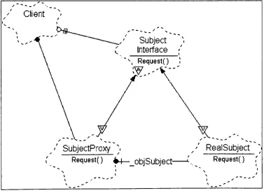
3.3.2.2
Proxy
36
3.3.3 Behavioral
Patterns
37
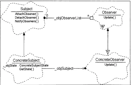
3.3.3.1 Observer
37
3.3.3.2
Strategy
38
3.4 TSPLIB 95
39
3.5
Primary
Packages
39
3.5.1
Basic GA
package40
3.5.1.1 Chromosome
Classes
40
3.5. 1.2
GA
Utility
Classes
41
3.5.1.3
GA
Resource
Classes
43
3.5.1.4
Selection Method
Classes
43
3.5.1.5 Crossover Method
Classes
44
3.5.1.6
GA
Style Classes
44
3.5.1.7
GA
Package
Summary
46
3.5.2 Basic CGGA
package47
3.5.2.1
Support Objects
47
3.5.2.2
Deme Objects
48
3.5.2.3 Master
Objects
49
3.5.2.4 CGGA Package
Summary
51
3.5.3
GA2 Package
51
3.5.3.1
Supervisory
GA
Classes
51
3.5.3.2 GA2 Deme Classes
51
3.5.3.3 GA2 Master Classes
52
3.5.3.4 GA2 Package
Summary
52
3.5.4 Thesis Package
52
3.5.4.1 Thesis Utilities
52
3.5.4.2 Thesis Serial GA
53
3.5.4.3 Thesis Master Classes
53
3.5.4.4 Thesis Deme Classes
54
3.6
Supporting
Packages
.55
3.6.1
awt.
55
3.6.2
lang
55
3.6.3
io
56
3.6.4
math58
3.6.5
net59
4. Data
andAnalysis
61
4.2 Basic Coarse-Grained Genetic Algorithm
65
4.3 Non-Uniform Distributed
Genetic
Algorithm
67
4.4 Adaptive Distributed
Genetic
Algorithm
68
4.5 Side-By-Side
Comparison
75
5.
Conclusions
77
5.1 Future
Code
Development
77
5.2 Future Research Areas
78
List
of
Figures
FIGURE
1
:THE BASIC GA
SEQUENCE
3
FIGURE
2: BASIC ROULETTE
WHEEL
SELECTION ALGORITHM
8
FIGURE
3: RWS
WITH
RANK SCALING
EQUATION
8
FIGURE
4: RWS
WITH
SIGMA SCALING EQUATION
9
FIGURE
5: SINGLE
POINT
CROSSOVER EXAMPLE
10
FIGURE
6:
DOUBLE POINT
CROSSOVER EXAMPLE
1 1
FIGURE 7: UNIFORM
CROSSOVER
EXAMPLE
1 1
FIGURE
8: CYCLE CROSSOVER EXAMPLE
13
FIGURE
9: ORDERED CROSSOVER EXAMPLE
14
FIGURE 10: PARTIAL
MATCHED CROSSOVER
EXAMPLE
15
FIGURE
1 1
:EXAMPLE GLOBAL
PARALLEL
GA
19
FIGURE 12: EXAMPLE
COARSE-GRAINED
PARALLEL
GA
20
FIGURE 13: EXAMPLE
FINE-GRAINED
PARALLEL
GA
23
FIGURE
14:
A
GOOD GA2 FITNESS
FUNCTION
25
FIGURE 15: EXAMPLE FACTORY METHOD PATTERN BOOCH DIAGRAM
33
FIGURE
16: EXAMPLE SINGLETON PATTERN BOOCH DIAGRAM
34
FIGURE 17:
EXAMPLE
CLASS
ADAPTER PATTERN BOOCH DIAGRAM
35
FIGURE 18: EXAMPLE OBJECT ADAPTER PATTERN BOOCH DIAGRAM
35
FIGURE
19:
EXAMPLE
PROXY PATTERN BOOCH DIAGRAM
36
FIGURE 20: EXAMPLE OBSERVER PATTERN BOOCH
DIAGRAM
37
FIGURE 21
:EXAMPLE STRATEGY PATTERN
BOOCH
DIAGRAM
38
FIGURE
22:
SAMPLE INI FILE
57
FIGURE
23: SAMPLE TSP DATA FILE
(ATT48.TSP)
58
FIGURE 24: ATT48 WITH TSPLLB OPTIMAL TOUR
61
FIGURE
25:
SERIAL
GA SCORES
63
FIGURE
26:
ATT48 SERIAL
GA
SEED 100109 TOUR
64
FIGURE
27:
SERIAL AND
CGGA
SCORES
66
FIGURE
28:
SERIAL AND NUDGA
SCORES
68
FIGURE
30:
GA2 TOURNAMENT
SIZES
FOR SEED 100049
70
FIGURE 31: GA2 POPULATION
SIZES
FOR SEED 100049
71
FIGURE
32:
GA2 MUTATION
RATES
FOR SEED 100049
72
FIGURE
33:
GA2 MIGRATION RATES FOR SEED 100049
73
FIGURE
34:
GA2
CROSSOVER
METHODS FOR SEED 100049
74
FIGURE
35:
SERIAL AND
GA2 SCORES
75
List
of
Tables
TABLE
1
:KEY
SERIAL
GA
STATISTICS
62
TABLE
2:
KEY
CGGA STATISTICS
65
TABLE
3:
KEY NUDGA
STATISTICS
67
TABLE 4: BEST NUDGA PARAMETERS
67
TABLE
5:
KEY
GA2 STATISTICS
69
Glossary
Note:
All
significantterms
first
appear as underlinedtext
in
the
mainbody
ofthis thesis.
Term
Page
Definition
1
ATSP
1
Asymmetric
Traveling
Salesman Problem
CGGA
20
Coarse-Grained Genetic
Algorithm
deme
20
A
nodein
aCGGA
EA
3
Evolutionary
Algorithm
Elitism
17
A
technique
for
forcibly
retaining
individuals
withina populationFGGA
22
Fine-Grained
parallelGenetic
Algorithm
Fitness
Sharing
18
A
technique
for reducing
premature convergenceGA
3
Genetic
Algorithm
GA2
24
Adaptive distributed Genetic Algorithm
GARAGe
23
Genetic Algorithm Research
andApplications
Group,
Michigan
State
University
iiGA
25
Island-Injection
Genetic
Algorithm
JVM
29
Java
Virtual Machine
L
5
Chromosome
length
NP-Complete
1
Nondeterministic Polynomial Complete
NUDGA
24
Non-Uniform
Distributed
Genetic
Algorithm.
Population
Crowding
18
A
technique
for
reducing
premature convergenceRMI
30
Remote Method Invocation
RPC
30
Remote
Procedure Call
RWS
7
Roulette Wheel
Selection
Schema
orSchemata
6
Useful
information encoding
blocks for
analyzing
genetic operatorsSTSP
1
Symmetric
Traveling
Salesman Problem
TCP/LP
32
Transfer
Control Protocol/Internet Protocol
TSP
1
Traveling
Salesman
Problem
URL
77
Uniform Resource Locator
1. Introduction
Of
significanceto the
computerengineering
community
arethe
optimalrouting
problemsrelated
to the
design
andlayout
ofVery
Large-Scale
Integrated Circuits
(VLSD.
Designs
with shorttraces
andfew
vias resultin layouts
that
are morereliable,
lower
cost and easierto
maintain or rework.While
not aVLSI
layout
problem,
Traveling
Salesman
Problems
(TSPs)
are a class of similar problemsthat
areNP-Complete.
Algorithms
ableto
solve aTSP
canbe
adaptedfor
VLSI
layout
problems.This
thesis
specifically
workswith
Symmetric
Traveling
Salesman Problems
(STSP).
These
areTSP
problems wherethe
distance
(or cost) between
two
citiesis
the
same whentraveled
from
city 1
to
city
2
as when
traveled
from
city 2
to
city
1.
An Asymmetric TSP
(ATSP)
is
a problem wherethe
distance
(or cost)
between
two
citiesis
notthe
same.A
genetic algorithmis
atechnique
for achieving
a problem's solutionthrough
anindirect
means.
Randomly
generatedinformation
that
encodes potential solutionsis
manipulatedby
softwaremodels of natural genetics and evolution.The
outcomeis
the
generation ofencodedsolutions
that
arecontinually
improved. Genetic
algorithmsare often placedin
the
role of optimizerfor
problemsthat
aretoo
difficult for direct
analyticaldevices.
However, they
have
alsobeen
successfully
appliedin
many
other areasincluding
classifier systems(the
abstraction ofcomplementary
rulecollections)
andthe
development
of antibodiesto
antigens[SFP93,
p.145].
Coarse-grained
parallel genetic algorithms are extensions ofthe
basic
serial algorithm.Multiple instances
ofthe
serial algorithm are executedconcurrently
with periodiccommunication
between
the
instances
to
exchangebest
know
sets of genetic material.The instances
areeffectively
isolated for
a period oftime
allowing
independent
development
of their own genetic material.The information
exchange updates eachinstance
with new andpossibly
different
materialthat
may
allowthe
instance
to
moreallows more of
the
fitness landscape
to
be
examined at onetime
as comparedto
the
serial algorithm.This
paper comparesthe
ability
offour
genetic algorithmimplementations
to
solve aninstance
oftheTraveling
Salesman
Problem,
ATT48
from
the
TSPLLB
archive[TSPLLB].
The four implementations
are: a serial geneticalgorithm,
abasic
coarse-grained parallelgenetic
algorithm,
a non-uniformdistributed
genetic algorithm and an adaptivedistributed
genetic algorithm.The
later
two
implementations
are advancedderivatives
ofthe
basic
coarse-grained algorithm.It is
shownthat
whilethe
standard course-grainedparallel algorithm provides more consistent results
than
the
serial geneticalgorithm, the
adaptivedistributed
algorithmcanfind better
solutions even more consistently.Coarse-grained
parallel genetic algorithms canbe implemented
as adistributed
system.The
Java programming
language is
asimple,
interpreted,
object-orientedlanguage
developed
by
Sun Microsystems
that
is currently
popularfor
the
development
ofdistributed
systems.This
thesis
utilizedthe
Java programming
language,
andits
Remote
Method Invocation
features,
to
develop
anobject-oriented, reusable,
and extensibledistributed
coarse-grained parallel geneticalgorithmslibrary.
Section 2
ofthis thesis
presents a significantdiscussion
ofthe
essentialbackground
points
to
the
development
ofthis
thesis:
genetic algorithms and parallel genetic algorithm.Section
3 introduces
the
readerto
Java,
Remote
Method
Invocation,
and object-oriented softwaredesign
patternsthat
were usefulto the
development
ofthe
thesis' code.Additionally,
adiscussion
and overview ofthe
design
anddecisions
relatedto the
implementation
is
supplied.In
section4,
the
results ofthe
experiments onthe
developed
code are presented
along
with ananalysis ofthose
results.Finally,
section5
gives some2. Background
and
Theory
2. 1
Genetic Algorithms
Initial
researchinto
evolutionary
strategiesinvolved solving only
specific problemswithout consideration as
to
how
these
strategiesactually
worked.After
adecade
ofdevelopment,
John
Holland
officially
introduced
genetic algorithmsin
1975
as"an
abstraction of
biological
evolution."
[MM96,
pp.2,
3].
It
washis intent
to
create aformal
methodby
whichto
study evolutionary
strategies.The
generalEvolutionary
Algorithm
(EA)
uses asexual reproduction[MH90,
p.2].
For
example,
Simulated
Annealing
(SA)
implementations
typically
executeusing
a single solution(a
populationsize of
one)
whichis
mutatedinto
anotherindividual
whois
scoredusing
some measurementfunction. The
newindividual is
acceptedto
replacethe
originalindividual
based
upon some predefinedprobability
function.
The probability
function
typically
varies with
the
length
oftime
ofthe
run.This
variance often allowsthe
rejection of good newindividuals early in
the
run whilelater accepting
only
the
very
best.
In contrast,
the
Genetic
Algorithm
(GA)
usesmodels of sexualreproduction;
a number of parents(two
ormore)
creates a number of children(one
or more).The individuals (a
population size greaterthan
one)
are evaluatedfor
their
fitness
toward
solving
a problem.Some
individuals
(also
calledchromosomes)
are selectedfor
reproductionto
createthe
nextgenerationof
the
population.Most
genetic algorithms usethe
samebasic
step
sequence:1.
Randomly
initialize
the
population.2.
Score
the
population(or
newestindividuals
ofthe
population).3
.Check for
termination
criteria.4.
Select individuals for
crossover.5.
Crossover
those
selected(reproduce).
6.
Mutate
those
created(if desired).
7.
Select individuals for
replacement.8.
Repeat
from
step
2.
There
aremany
variations ofnearly every step
in
the
process.For
a particular run of a geneticalgorithm,
a selectionfrom
these
variants mustbe
made.Collectively,
these
variations are called
the
genetic algorithm's parameters.A
poor choice of parameters can slowthe
GA's
convergence rate anddiminish
the
final
quality
ofits
solution.Before these
steps canbe
taken,
severalimportant
questions mustbe
addressed:1
.How
is
the
fitness
of anindividual
ofthe
population scored?2.
What
arethe termination
criteriafor
the
algorithm?3.
What is
the
solutionrepresentationfor
that
problem?2.1.1
Fitness
Evaluation Functions
The
function
that
evaluates a given chromosomefor its fitness
atsolving
the
problem athand
is
one ofthe
mostdifficult
to
write.There
arevery
few
guidelinesfor
writing
goodfitness functions (and fewer
still onhow
to
avoidwriting
bad
ones).Improperly
writtenfitness
functions
caneasily
maskthe
use of otherwise acceptableGA
parameters.GAs
use
the
score returnedby
the
fitness functions
to
determine
the
relative merits ofthe
chromosomes with respect
to the
rest ofthe
population.Individuals
withbetter
scorestend to
be
rewardedby
remaining in
the
populationlonger
andby
being
giventhe
opportunity
to
produceoffspring."Better"
depends
upon whatthe
problemis.
Analytic
functions
arethe
most straightforwardfitness functions. Once
the
chromosomeis decoded into
valuesfor
each variablethey
canbe
"plugged"into
the
function.
The
fitness is
then
the
final
solutionto
the
equation(s).The
fitness function for
otherproblems
depends
directly
uponthe
chromosomerepresentation.2.1.2
Termination
Criteria
The
teraiination(or exit)
criterionfor
a genetic algorithm varies withthe
intent
ofthe
check
may
be
performed,
andthe
programis
forcefully
terminated
viathe
operating
system whendesired.
In
the
samecontext,
a maximalboundary
may
be
establishedto
limit
the
duration
ofthe
algorithm run.Alternatively,
analysis ofthe
genetic algorithm's runtime statisticsmay
yield usefulinformation
for
determining
whenit is
"done."
At
this
point,
the
algorithm canbe
terminated
gracefully.One
examples ofthis
is
whenthe
average rate of progress(movement
towards the
globaloptima)
falls
below
a giventhreshold
(i.e.
it has found
alocal
optima).In
this case, the
GA is
unlikely
to
do
any
better
than
it
has,
asit is
notmaking any
significantimprovement.
This
could alsobe
measured
by
adecrease in
the
variance ofthe
population members.2.1.3 Problem Representation
When using
a geneticalgorithm,
it is
necessary
to
decide
whatinformation is
to
be
encoded vrithin
the
chromosome.The
encodedinformation is
problemdependent.
If
the
probleminvolves
optimizing
an analyticfunction,
the
chromosomemay
be
one or more coordinates or variable values.For example,
afunction
oftwo
variables might encodethe
X
andY
coordinates each as16
bit fixed
pointdecimal
values.A
bit
chromosome(a
chromosome of anarbitrarily
long
string
ofbits)
oflength
32
might encodethe
first
16
bits
asthe
X
coordinate andthe
last
16
bits
asthe
Y
coordinate.If the
problemis
anordering
problem,
such as abin packing
or atraveling
salesmanproblem,
the
chromosomemay
be
a sequence ofintegers
indicating
whichbin
orcity
is
to
be
used next.The
population might consist of arrays ofintegers,
eachinteger
having
a value[0..L).
'L'denotes
the
size ofthe
chromosome.Some
problemsmight not utilize such uniform chromosome encodings.With
abit-based
2.1.4 Schema
Theory
"The
mostdifficult
partof
a random search methodis
toexplainwhy
and whenit
willwork."
[MH91,p2]
Schema
Theory
is
usedto
describe
and predict some parts ofthe
behavior
of genetic algorithms.Schema
are sequences ofinformation
withina chromosome'sencoding
that
representthe
"building
blocks"of a solutionto the
problembeing
solvedby
the
genetic algorithmThese
sequences aredescribed
using
bit
strings ofones,
zeros and asterisks(for
"don't
cares").For
examplethe
string
1
* * * *0 is
representative of all six-bit stringsbeginning
with a one andending
in
a zero.Schema
are classifiedby
length
and order.The
length
of schemais
the
distance between
the
first
non-asterisk ofthe
pattern andthe
last
non-asterisk ofthe
pattern.The
order of schematais
the
number of non-asterisksin
the total
pattern.For example,
the
schemata***l
i
* *q o
* *has
alength
of six with an order offour.
Schema
theory
is
very
applicableto
predicting
andexplaining
the
effects ofthe
crossover operators.Although
schema patterns aredescribed
using
ones andzeros, the
schema patterns are notstrictly
bit string
patterns.These
patternsapply
to
all chromosometypes
and caneasily
be
applied asindex
masks onto chromosomefield indices.
2.1.5 Initialization
andPopulation
Sizing
The initialization step
involves
iterating
through
each member ofthe
population andrandomly
filling
in
their
genetic material.How
this
is done depends
uponthe
chromosomeitself.
If
the
chromosomeis
abit
representation,
eachbit
mustbe
individually
set(or
cleared).If
instead
the
chromosomeis
a primitivedata
type
(e.g.
aninteger
orfloating
pointdata
type)
each genein
the
chromosome cantypically
be
setdirectly
from
the
local
random number generator.size
is
integrally
linked
to
the
selection andcrossovermethods andis difficult
to
specify
correctly
for
anarbitrary
problem.In
general,
smaller population sizestend
tobecome
homogenous
morequickly
than
larger
populations.This
is believed
to
be
a side-effect ofthe
crossover method nothaving
enough genetic materialto
work withbecause
ofthe
inability
ofthe
populationto
adequately
samplethe
problemdomain.
However,
the
effectiveness ofthe
crossover methodis
reduced withthe
use of"large"
populations
(the
crossovermethod
discussion
is
in
section2.
1.7).
Suffice
to
say
the
population musthave
sufficient(statistically
significant)
coverage ofthe
building
blocks
of a good solution.Without
this,
aGA
has little
probability
ofarriving
at aquality
solution.2.1.6
Selection
Methods
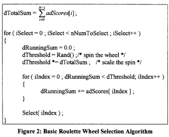
2.1.6.1 Fitness Proportional
Selection
N-l dTotalSum=
i=0
for
(
iSelect
=0 ;
iSelect
<nNumToSelect; iSelect++
)
{
dRunningSum
=0.0 ;
dThreshold
=Rand()
;/*spin
the
wheel*/
dThreshold
*=dTotalSum
;
/* scale the spin*/
for
(
ilndex
=0
;
dRunningSum
<dThreshold;
ilndex-H-)
{
dRunningSum
+=adScores[
ilndex
]
;
}
Select(
ilndex
)
;
Figure
2: Basic
Roulette Wheel
Selection
Algorithm
There
aretwo
common modificationsto the
RWS
algorithmthat
reducesits
selectionpressure: rank
scaling
and sigma scaling.Both
have
the
effect ofreducing
the
merit ofany
singleindividual
with respectto the
population as a wholethus
evening
outthe
probability
of selectionfor
each chromosome(reducing
the
overall selectionpressure)
anddecreasing
the
convergence rate ofthe
GA.
RWS
with rankscaling
modifiesthe
fitness
scores usedby
the
basic RWS
algorithmby
replacing
each chromosome's score with a value(0
to
L-l). Each
chromosome's scoreis
indicative its
relative rank comparedto the
rest ofthe
population.The
following
equation
details
the
scaling:Vi
\adNewScores[i]
=dMinScore
+(dMaxScore
-dMinScore)
Rank(i)-\
JV-1
[image:21.553.110.440.55.323.2]RWS
with sigmascaling
also modifiesthe
scoresthat
are usedby
the
basic
RWS
by
replacing
the
each chromosome's score withthe
output ofthe
following
equationbased
on
the
standarddeviation
ofthe
population(a):
If
ais
not equalto
0
Vi\adNewScores[i]
=1
+adScores[i]
-adScores
Otherwise
V
'i\adNewScores[i]
=1
Figure
4:
RWS
withSigma
Scaling
Equation
2.1.6.2 Tournament
Selection
An
alternativeto
the
classicRWS
methodis
the
Tournament
Selection
method.This
method
is
somewhat simplerthan the
RWS
method.A
tournament
is
"held" amongst arandomly
selected sample ofindividuals
ofthe
population.The
tournament
selectsthe
mostfit
individual
ofthe
samplefor
reproduction.The
tournament
size(x)
has
clearimplications
uponthe
selection pressure ofthe
GA.
The
larger
the
tournament,
the
greater
the
pressure onthe
populationto
converge.A
tournament
size of oneis
atotally
randomselection method.A
tournament
size oftwo
has
properties similarto
RWS
with rank scaling.For
this
size and alltournament
sizesgreater,
anindividual's
scoreis
irrelevant
to
its
selection.Instead,
only
its
rank withinthe
population as a wholeis
considered.
Lesser
rank will always "lose"to
higher
rank.Duplicate
scores are resolved arbitrarily.Larger
tournament
sizes are more elitistin
nature.This
increases
the
probability
ofthe
best individual in
the
populationbeing
selected andthereby
increasing
the
selection pressure ofthe
GA.
2.1.7
Crossover
Methods
Crossover
is
the primary
mechanismby
which genetic algorithms create new(and
more parents
to
create one or more children.There
aremany
different
crossovermethods available.
Some
are generalpurpose,
others problem specific.The
"normal"biological
rulesfor
sexual reproduction need notapply
to
these
methods.One
or moreparents can generate one or more children.
It
is
strictly up
to the
user or programmer.Often,
atleast
two
parent chromosomes are selectedto
create one ortwo
childchromosomes.
This
thesis
only
utilizes anddiscusses
crossover methodsthat
involve
two
parentsyielding
two
children.2.1.7.1
Bit
Crossover
Methods
Perhaps
the
most commonbit
crossover methodis
single point crossover.A
randompoint
(p)
is
selectedalong
the
length
oftwo
parent chromosomes.The
first
oftwo
childrenis
createdfrom
the
parentsby
copying
parentl[l..p]
to
childl[l..p]
andparent2fp+l..NJ
to
childl[p+l..NJ.
Similarly,
the
second childis
createdby
copying
parent2[l..p]
to
child2[l..p]
and parent1
[p+l..NJ
to
child2[p+l..N].Schema
analysis of single point crossoverindicates
that this
crossover methodtends to
preservelonger
schemata(compared
to
double
point and uniform crossover).Single
point crossover atindex
3
Parent
1
is
Parent 2
is
Child
1
becomes
Child 2 becomes
AAA
|
BBBBBB
CCC|DDDDDD
AAA|DDDDDD
CCC I BBBBBB
Figure 5: Single
Point
Crossover Example
A
similar methodis double
point crossover.Instead
of a single crossoverpoint,
two
crossover points are selected.
Two
children are createdby
copying
each parentdirectly
into
a child chromosome andswapping
the
inner
substring
delineated
by
the two
Double
point crossover atindexes 3
and7
Parent 1
is
AAA
|
BBBB
|
CC
Parent 2
is
DDD|EEEE|FF
Child
1
becomes
AAA|EEEE|CC
Child 2 becomes
DDD
|
BBBB
|
FF
Figure 6:
Double Point
Crossover
Example
It is
nothard
to
rationalize aK-point
crossover method(where 0<K<N).
As
K^> N
,the
crossover method will preserveprogressively
smaller schema.The
uniform crossover method preserves smaller schemain
a manner similarto
ahigh-order
K-point
crossover method(where
K
->N).
Two
children are createdby
iterating
through the
length
ofthe
chromosome andcopying
bits into
the
childrenfrom
the
parentFor
eachbit
position,
a random numberis
generated andthresholded.
If
the
value
is
overthe
threshold,
the
bits
are copieddirectly
into
the
childrenfrom
the
associated parent.
If
the
valueis less
than the
threshold,
the
bits from
the
parents areswapped
before
being
writteninto
the
children.Parent 1
is
AAAAAAAAA
Parent
2
is
BBBBBBBBB
Child
1
becomes
BABAAABAA
Child 2 becomes
ABABBBABB
Figure 7:
Uniform
Crossover
Example
Research
into
the
usefulness of uniform crossoverhas
shownthat there
aretwo
specificsituations where
it
willtend to
out-performboth
the
single ordouble
point crossover methods:1.
During
the
end ofthe
GA's
run,
whenthe
populationtends to
be
morehomogeneous,
push
the
populationfurther.
This
canbe likened
to the
effect of mutation(section
2.1.8).
2.
When
a run uses a population sizethat
is
too
smallfor
adequate coverage ofthe
searchable space.
The
disruption
causedby
the
uniformcrossover operator can"help
overcome
the
limited information
capacity
of smaller populations andthe
tendency
for
morehomogeneity."
[DJS90,
p.8]
2.1.
7.2 Permutation-Based
Crossover Methods
For
chromosomesthat
encodepermutations,
it
is
not possibleto
randomly
change valuesin
the
chromosome.To
do
so woulddisrupt
the
uniqueness ofthe
chromosome's genes.The
following
crossover methods each provide adifferent
way
ofrecombining
the
genesof
two
parentchromosomesto
generatetwo
new anddifferent
(usually)
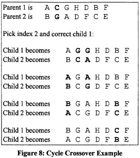
children.Cycle Crossover
creates child chromosomesby
first
copying
each parentinto
one ofthe
childrenand
then
randomly
interchanging
one ofthe
genes.Since
the
chromosomes areunique, this
interchange
creates a redundant genein
each ofthe
child chromosomes.The
cycle crossover method gets
its
namefrom
how
it
resolvesthis
duplication;
it
choosesone of
the
child chromosomes and searchesfor
the
newly
duplicated
gene.When
found,
that
index is
alsointerchanged
withthe
other child chromosome.This
secondinterchange
may
removethe
duplication
orit
may
introduce
adifferent duplicate
gene.Cycle
crossover repeatsthis
process onthe
selected child chromosome until eitherthere
is
no moreduplication
orthe
original parent chromosomes are recreated.Schema
analysis showsthat
cycle crossover can preserve anddestroy
both
short andlong
Parent 1
is
A
C
G
H
D
B
F
Parent 2
is
B
G
A
D
F
C
E
Pick
index
2
and correct child1
:Child
1
becomes
A
G
G
H
D
B
F
Child
2
becomes
B
C
A
D
F
C
E
Child 1
becomes
A
G
A
H
D
B
F
Child 2 becomes
B
C
G
D
F
C
E
Child
1
becomes
B
G
A
H
D
B
F
Child
2
becomes
A
C
G
D
F
C
E
Child
1
becomes
B
G
A
H
D
C
F
Child 2
becomes
A
C
G
D
F
B
E
Figure
8: Cycle
Crossover Example
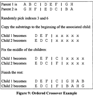
Ordered
Crossover
worksdifferently
from
cycle crossover.The
ordered crossovermethod selects
two
randomindexes
to
create asubstring
from
each parent chromosome.Each
substring is
copiedinto
the
beginning
ofthe
associated child chromosome.The
middle of each child chromosome
is
constructedby
appending any
non-duplicate genefrom
the
other child chromosome.The
remainder of each child chromosomeis
generated
by iterating
through
the
parent chromosomestarting
to
theright
ofthe
substring
(using
modulo arithmeticif
necessary)
andappending any
genesthat
do
not [image:26.553.156.397.48.319.2]Parent 1
is
A
B
C
|
D
E
F
I
G
H
Parent 2
is
G
H
F
|
E
D
C
|
B
A
Randomly
pickindexes 3
and6
Copy
the
substringsto the
beginning
ofthe
associated child:Child
1
becomes
D
E
F
X X X X XChild 2 becomes
E
D
C
X X X X XFix
the
middle ofthe
children:Child
1
becomes
D
E
F
C
|
X X X XChild 2 becomes
E
D
C
F
|
X X X XFinish
the
rest:Child
1
becomes
D
E
F
C
I
G
H
A
B
[image:27.553.126.426.47.366.2]Child 2
becomes
E
D
C
F
|
B
A
H
G
Figure 9: Ordered Crossover Example
Schema
analysis of ordered crossover revealsthat
schemata short enoughto
exist withinthe substring
willbe
preserved while all other schema willtend to
be destroyed.
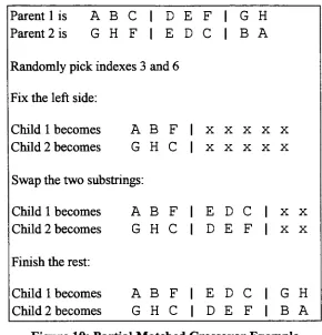
Partial Matched
Crossover
(PMX)
providesfunctionality
that
is
a combination ofthe two
previous methods.
Like
orderedcrossover, two
randomly
located indexes
are usedto
mark substrings oftwo
parent chromosomes.The left
portion of each childis
createdfrom
checking
for
the
existence of each parent'sleft
genesin
the
opposite parent'ssubstring.
If
a geneis
found,
the
genein
the
child's associated parent'ssubstring
atthe
sameindex is
used.Otherwise,
the
geneis
copieddirectly
into
the
child.The right
portion of each childis
formed
similarly.The
middle portion of each childis formed
by
copying
the
opposite parent'ssubstring
into
the
child.PMX
effectively
preservers entire schema as ordered crossoverdoes but
alsodisrupts
preserve useful schema while
pushing
the
populationforward
viathe
recombination ofother more
marginally
preserved schema(those
partially
destroyed
by
the
Cycle-like
activities).
Parent
1
is
A
B
C
|
D
E
F
I
G
H
Parent
2 is
G
H
F
|
E
D
C
|
B
A
Randomly
pickindexes
3
and6
Fix
the
left
side:Child
1
becomes
A
B
F
X XXX XChild 2 becomes
G
H
C
X XXX XSwap
the two
substrings:Child
1
becomes
A
B
F
E
D
C
|
X XChild
2
becomes
G
H
C
D
E
F
|
X XFinish
the
rest:Child
1
becomes
A
B
F
E
D
C
|
G
H
Child 2 becomes
G
H
C
D
E
F
|
B
A
Figure
10:
Partial
Matched
Crossover
Example
Other
crossover algorithms existfor
specific probleminstances.
Maximal
Preservation
Crossover
(MPX)
has
specifically been
developed for (and
successfully
appliedto)
solving
Traveling
Salesman Problems
[MH91,
p.331]. Its intent is
to
maintain subtourscommon
between
two
parentchromosomes.(This
thesis
has
chosen notto
investigate
the
applicationand
development
of problemspecific crossover methods.Rather,
its focus is
on
the
benefits
ofdifferent
parallel genetic algorithmimplementations.)
2.1.8 Mutation
Mutation
is
the
mechanismwhereby
the
genetic algorithm extendsits
current genetic [image:28.553.128.418.134.436.2]towards
whichthe
populationis
currently
climbing.Mutation
is
often considered anoptional
step in
the
generalGA
process.It
is
suggestedthat
given asufficiently large
population,
enough coverage ofthe
problemdomain
canbe
made suchthat
crossoverby
itself
cansufficiently
arrive atthe
best
solution.While
this
may
be
true
for
smallerproblems,
problems ofany
"real-world" size would require populationsthat
areimpractical
to
work with.The
GA
parameterPm
is
usedto
signify
the
percentage ofgenes of a specific chromosome
that
are selectedfor
mutation.2.1.8.1 Bit Chromosome Mutation
For
bit-based
chromosomes, the
concept of mutationis
straightforward.Multiply
Pm
by
L
to
getthe
number of genesto
mutate(M).
For
allM,
randomly
select a genefor
mutationand
randomly
resetthe
bit
value.The
newbit
value canbe
obtainedby
thresholding
avalueextracted
from
a random number generator.The
threshold
is
usedto
determine
the
binary
value ofthe
newbit.
Commonly
setto
50%,
the threshold
canbe
placedanywhere
in
an attemptto
bias
mutationtowards
a certain outcome.2.1.8.2 Permutation Chromosome
Mutation
Simple integer
chromosomes canbe
mutatedin
a manner similarto the
bit
chromosome.Instead
ofchanging
abit,
acompletely
newinteger is
extractedfrom
the
local
randomnumber generator
to
replacethe targeted
gene.This
method canpotentially
resultin
the
duplication
of values.Permutation
representative chromosomes require a slightmodification
to the
mutation concept.Since only
oneinstance
of each geneis
allowedto
exist
in
the
chromosome,
randomly
changing
a gene's value would resultin
the
duplication
ofanexisting
gene.This
is obviously
undesirable.Instead,
the
mutation rate(Pm)
is
divided
by
two
to
createthe
modified mutation rate Pmn,.Pmm
is
multipliedby
L
to
get
the
number of genesto
mutate(M). For
allM,
anindex
randomly
selectedto
mutate.A
newvalueis
generatedfor
this
gene andthe
chromosomeis
searchedfor
the
index
ofthe
genethat
has
this
newly
obtained value.When
located,
the
two
genes are swapped.The
normal mutation rateis halved because
this
mutationalgorithm changestwo
genes2.1.9 Replacement Policies
2.1.9.1
Generational
The
classicGA
creates anentirely
new populationfrom
the
repetitive selection ofmembers
from
the
original population.This is
considered a generational modelbecause
each new populationis
consideredto
be
ageneration.Variations
of thispolicy
exist.A
common variant
is
the
replacement ofonly
some percentage ofthe
population.The
replacement percentage
is indicated
by
pr.Often,
pr
*N
(where
pr
is
small)
is
replacedinstead
ofthe
entirepopulation,
andthose
replaced arecommonly
the
least fit individuals
of
the
population.Another
variant accommodatesthe
lack
of preservationby
the
selection methods.
Elitism
forcibly
requires some percentage ofthe
best individuals in
the
populationto
be
retainedinto
the
next generation.While
elitismnormally
retainsonly
one or afew
individuals,
this
value could alsobe
viewed as alarge
replacement percentage.The
classicGA
replacement model couldsimilarly
be
stated as100%
replacement or0%
elitism.2.1.9.2
Steady-State
Instead
ofreplacing
the
entire population atonce,
the
steady-stateGA
replacesonly
afew
individuals
at atime.
This
helps
maintainstability
withinthe
population and resultsin
abuilt-in
elitism.The best individual
of a population will neverbe
selectedfor
replacement.
Additionally,
this
mechanismdoes
nothave
"generations"
of
individuals.
Subsequently
it is
not possibleto
compare a steady-stateGA
directly
to
a generationalGA.
Instead,
comparisons mustbe based
uponthe
number offitness
evaluations orfitness
comparisons executedby
the
algorithm.In
this way, the
relative merits of eachGA
type
canbe
analyzed.This
policy
allowsfor
abuilt-in
niching
mechanismbecause
the
selection of replacementindividuals
usually
involves
the random,
but
directed,
selectionof
lesser fit individuals.
2.1.10 Premature
Convergence
One
ofthe
most significant problemsfacing
the
GA community
is
the
prematurea significant component of
the
success of genetic algorithms.The
fitness
proportionalGA "assigns exponentially
increasing
numbers oftrials to the
observedbest
parts ofthe
search
space."
[SFP93,
p.128]
This ability
comprises much ofthe
GA's
capacity
tosolve problems.
At
the
sametime,
this
can restrictits ability
to
search a solution spaceby
reducing
the total
amount ofgenetically
diverse
materialin
the
population.Typically,
an effort
to
reducethe
possibility
of premature convergence also slowsthe
convergencerate of
the
GA
in
general.This
is
usually
accomplishedby
reducing
the
selectionpressure of
the
GA.
A
trade-off, then,
existsbetween
the
needto
find
a good solutionquickly,
andthe
slowing
ofthe
convergence rate ofthe
GA
(which improves
the
potentialof
creating
an evenbetter individual
that
might not otherwisebeen
realized).Algorithms
to
reducethe
seriousness ofthis
problem abound.DeJong
introduced
the
concept of
Population
Crowding
in
1975
[SFP93,
p.129].
After
creating
a newindividual
for
the population,
anindividual is
selectedfor
replacementby
first
randomly
drawing
of some percentage ofthe
population andthen
determining
which ofthe
members of
the
drawing
mostclosely
resemblesthe
newindividual.
This
schememaintains genetic
diversity
by
enforcing
the
"uniqueness" of each member ofthe
population.
Crowding
is
typically
implemented in
a steady-stateGA (see
section2.1.9.2). Fitness
Sharing
works similarly.However,
it
penalizes newindividuals for
the
existence of population members similar
to them.
The
usefulness offitness
sharing
canbe limited
by
the
loss
of genetic material withinthe
population as an effect ofthe
selection and crossover methods.
This
canbe
compensatedfor
by
increasing
the
population size.
Unfortunately,
fitness
sharing
is
an orderN
algorithmrequiring rapidly
increasing
amounts oftime.
The
determination
ofthe
penaltiesfor
fitness
sharing
alsorequires
knowledge
ofthe
problemdomain
that
may
notbe
available.Fitness sharing
can still
be
useful,
however,
because it does
force
the
existence of stable niches rather2.2
Parallel
Genetic Algorithms
There
arethree
major categories of parallel genetic algorithms:global, coarse-grained,
and
fine-grained.
This
section presents an overview of eachtype
along
with severalalternative
designs originating
as coarse-grainedGAs.
2.2.1
Global Parallel
Global
Parallel
(or
Panmictic)
Genetic Algorithms
areimplementations
that
strictly
areparallelizations of
the
serialGA.
Assuming
afitness
proportionate selection method(see
section
2.1.6.1),
the
fitness
evaluations and mutation ofindividuals
ofthe
population'snext generation can all
be done
in
parallel.A
bottleneck in
the
parallel algorithm occursonly
whenit is
necessary
to
calculatethe
population's averagefitness
value andto
sumthe
entire population's fitness'With
someplanning,
selection,
crossover andreplacement can also
be done in
parallel.The
benefits
ofthese
implementations,
however,
are notnecessarily
worthwhile.The
genetic operators(e.g.
crossover,
selection,
mutation)
are quitesimple,
andit
shouldbe
expectedthat the
communicationoverhead required
to
parallelizethese
operators couldeasily
negate or penalizethe
speedup
or other performancegainsnormally
obtainedthrough the
parallelization effort.Nevertheless,
if
the
evaluation ofthe
fitness function is
computationally
intense,
globally
parallelGAs
are simpleto
implement
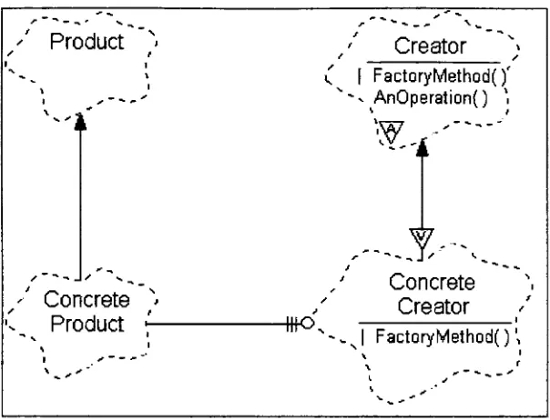
and canbe
more efficientthan
other parallelmethods.
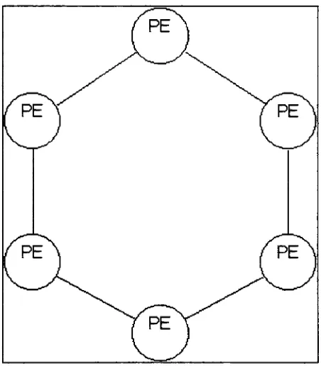
2.2.2
Coarse Grained Parallel
Coarse Grained
Parallel
Genetic Algorithms
(CGGAs)
are often referredto
asDistributed
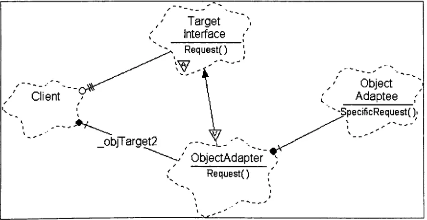
or
Island
Model
GAs. This
comesfrom
the
fact
that
CGGAs
are multiple serial genetic algorithmsrunning
independently.
The
separate serialGAs
are calleddemes.
All
[image:33.553.164.390.226.484.2]mutation, crossover,
and selection operations are performed aspreviously detailed in
section2.1.
Unlike globally
parallelGAs,
however,
the
genetic operators are appliedto
their
local deme
and notto
the
population as a whole.Figure 12:
Example
Coarse-Grained
Parallel
GA
A
connectiontopology
for
communication mustbe
establishedfor
the
variousdemes
ofthe
CGGA.
Often
static(although
not requiredto
be
so), the
connectiontopology
detennines
to
whatdemes
any
singledeme may
migrateindividuals
to
(including
itself).
The
intent is
to
allow eachdeme
to
movethrough
the
problemdomain
somewhatUnfortunately,
any
amount of migration willeventually
causethe
global populationto
converge.
CGGAs
have
three
additional parametersto
specify:the
migration rate,the
migrationinterval
and whether or notthe
demes
are synchronized atthe time
ofthe
migrationinterval (deme
synchronization).The
migration rateis
the
percentage ofthe
deme's
population
that
is
pushedto
each ofits
peerdemes.
A
value of0%
effectively isolates
alldemes
from
each other.That
is,
eachdeme develops
totally
independently
from
eachother.
It
is important
to
notethat the
percentage ofthe
populationpotentially
replaceddue
to
immigration
is
notthe
same asthe
emigration percentage.In
general, the
emigration rate
is
the
sum ofthe
number ofimmigrants from
each connectionto the
deme
(this
expression allowsfor
asymmetrictopologies
with uneven migration rates).The
connectivity
ofthe
demes has
alsobeen
the
subject ofdebate.
Some
studieshave
shown
that
ahigh
degree
ofconnectivity
between demes is best
while othershave
demonstrated
contrary
results.It
is
clearthat
afew
peers each with alarge
migration ratecan
easily
displace
the
entirelocal
populationin
a single step.Therefore,
the
migrationrate and network
topology
mustbe
carefully
considered.The
migrationinterval
determines
when eachdeme broadcasts its
emigrantsto
its
peers.Longer
intervals
alloweach population
to
develop
their
ownlocalized
niche ofthe
problemdomain.
The deme
synchronization parameterdetermines if
the
demes
stop
and waitfor
a "CONTINUE"signal after
broadcasting
their
emigrants.There
are severalimportant
characteristics
to
consider whensynchronizing
demes.
All
demes
develop
their
populations atthe
same rateallowing
for
an accuratetracking
andrecording
ofdeme
statistics.However,
if
aheterogeneous computing
network
is
utilized, the
benefits
ofthe
fastest
machine willbe
eliminated asthat
machine will
be forced
to
waitfor
the
slowest machineto
completeits
task.
Depending
onthe
implementation,
runs of synchronizeddemes
can oftenbe
aIt
is
possiblefor
the
deme implementation
to
know
that
allimmigrants have been
received oncethe
"CONTINUE" signalhas
been
received.Some
useful optimizationsmay
be
introduced
utilizing
this
fact.
When
the
demes
are not synchronized:Heterogeneous
networks are allowedto
workattheir
own pace:fast
machines are notlimited
by
slowermachinesmaximizing
the
effective ofthe
faster
machines.The
demes
arefree
to
evolvefreely.
It
is
notdependent
uponthe
reception of peer andtherefore
can continue asif it
wassimply
a serialGA
withinput from
other peers at an unquantifiableandpotentially varying
rate.If
ademe has
morethan
onepeer, the
recreation ofthe
runmay
be
impossible,
the
communications
delays
may
notbe
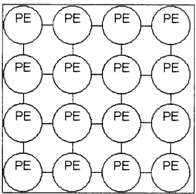
repeatable.2.23 Fine
Grained
Parallel
Fine Grained Genetic
Algorithms
(TGGAs)
are similarto the
CGGA
in
that
demes
are used andthe
genetic operators are appliedonly
atthe
deme level.
The
demes for
this
architecture are
small;
as small as possible.The
ideal
situationfor
aFGGA
implementations is
to
have
a singleprocessing
elementfor
eachindividual in
the
global population.In
this case, the
concept ofademe is
extendedto
become
aset of processors.These
parallelGAs
aretypically
implemented
onmassively
parallel machines.It
has
been
shownthat the
size and shape ofthe
deme
altersthe
overall selection pressure ofthe
GA. The
selection pressure canbe
directly
affectedby
the
ratio ofthe
radius ofthe
deme
/pe\
_/^pe\_/^pe\/pe\_
_/pe\/pe\
/pe\
_/^e\_/peY
[image:36.553.177.376.49.246.2](pe\
ypE\
_/pe\Figure 13:
Example Fine-Grained
Parallel
GA
2.2.4
Hybrids
Some
researchhas been focused
uponthe
combination ofthese three
classifications ofparallel
GAs.
Usually,
a small globalGA
or aFGGA
is
contained withinthe
deme
of alarger
CGGA
(less
commonly,
aCGGA
replacesthe
deme's
serialGA). The deme
gainsthe
benefits
ofthe
GA
modelthat
replacesthe
serialGA
andcorrespondingly,
the
CGGA
as a whole gains.
[CP971]
showsthat there
arelimits
to
the number ofprocessing
elementsthat
canbe effectively
utilizedby
aglobally
parallelGA
orby
aCGGA These
hybrids
are awady
to
utilize moreprocessing
elements withinthe
limitations
ofthe
respective
designs
andpotentially
improve
the
both
the
results obtained and convergencerate of
the
GA
Indeed,
hybrids
may
be
the
best
mechanismfor
solving very
large
problems.
The
CGGA deme does
nothave
to
be
aGA
at all.It
couldbe
aFinite Element
Analysis
(TEA)
algorithmthat
iterates
for
a period oftime
simulating
the
migrationinterval
or acompletely
separate nodethat
only
feeds
the
CGGA
newbest
solutions asit
finds
them.
A
combination ofFEA
and aCGGA has been
successfully
usedby
Michigan
State
University's
(MSU)
Genetic
Algorithms
Research
andApplications
Group
(GARAGe)
to
optimizethe
mass of a composite-basedflywheel
[ED97,
p.1].
The
results of
this
hybrid
approach(along
with otherGA
relatedinventions)
has significantly
2.2.5 Non-Uniform Distributed
The Non-Uniform Distributed
Genetic
Algorithm
(NUDGA)
attemptsto
improve
uponthe
basic
CGGA. For
mostproblems,
it is difficult
to
know
what parametersthe
geneticalgorithm needs
for
maximal efficiency.NUDGA
initializes
eachdeme
to
different
randomly
generatedGA
andCGGA
parameters.The
intent is
that
despite
the
lack
ofknowledge
ofthe
"correct"parameters,
some combination of mixed parameters willyield
better
resultsthan the
CGGA
withevery deme initialized
to the
same parameters.2.2.6 Adaptive Distributed
"An
EA,
whetherserial or parallelcanbe
effectiveonly
whenaproper
balance between
exploration(via
well chosenparameters)
andexploitation
(well
chosen selectionpressure)
is
maintained "[SDJ96,
p.236]
It
is
clearthat the
selection/optimization ofthe
GA
parametersfor
anarbitrary
non-trivialproblem
is difficult
particularly
because
ofthe
mutualinteractions
ofthe
parametersthemselves.
This
problemis
even more apparentif
the
problemdomain is
not wellunderstood.
The CGGA
is
simply
an extension ofthe
basic
GA;
adding
even moreparameters
to the
already
large
andvarying
setthat
arethe
basic
parameters.While
the
NUDGA
has
the
potentialto
achievebetter
resultsthan the
CGGA it
can(and
does)
choose sub-optimal parameter sets.
Having
no means ofidentifying
orcorrecting
those
poor
choices,
the
userbecomes
responsiblefor monitoring
the
progress ofthe
NUDGA
and
making
the
decision
to
prematurely
terminate the
experiment.The
Adaptive
Distributed
Genetic
Algorithm
(GA2)
extendsthe
NUDGA
by
this
one morestep; the
GA2
uses asupervisory
serialGA
to
measurethe
progress of eachdeme
andto
alterthe
parameters of specific
demes
whichit decides
to.
A
population size equalto
the
numberof
demes
is
utilized wherethe
chromosomes ofthe
supervisory
GA
encode eachdeme's
GA
andCGGA
parameters.All
GA
operators are exercised onthe
population.When
replacement
is
performed, the
demes
that
correspondto the
chromosomesbeing
replacedare sent
the
GA
andCGGA
parameters encodedin
the
new replacement chromosomes.Herein
lies
the
adaptive nature ofthe
GA2.
When
onedeme
significantly
outperf