The system science development of local time dependent 40 keV electron flux models for geostationary orbit

keV electron flux models for geostationary orbit.

White Rose Research Online URL for this paper: http://eprints.whiterose.ac.uk/146498/

Version: Accepted Version

Article:

Boynton, R.J. orcid.org/0000-0003-3473-5403, Amariutei, O.A., Shprits, Y.Y. orcid.org/0000-0002-9625-0834 et al. (1 more author) (2019) The system science

development of local time dependent 40 keV electron flux models for geostationary orbit. Space Weather. ISSN 1542-7390

https://doi.org/10.1029/2018sw002128

This is the peer reviewed version of the following article: Boynton, R. J., Amariutei, O. A., Shprits, Y. Y., & Balikhin, M. A. ( 2019). The system science development of local time dependent 40 keV electron flux models for geostationary orbit. Space Weather, which has been published in final form at https://doi.org/10.1029/2018SW002128. This article may be used for non-commercial purposes in accordance with Wiley Terms and Conditions for Use of Self-Archived Versions.

Reuse

Items deposited in White Rose Research Online are protected by copyright, with all rights reserved unless indicated otherwise. They may be downloaded and/or printed for private study, or other acts as permitted by national copyright laws. The publisher or other rights holders may allow further reproduction and re-use of the full text version. This is indicated by the licence information on the White Rose Research Online record for the item.

Takedown

If you consider content in White Rose Research Online to be in breach of UK law, please notify us by

The system science development of local time

dependent 40 keV electron flux models for

geostationary orbit

R. J. Boynton,1 O. A. Amariutei,2 Y. Y. Shprits,3,4 M. A. Balikhin,1

R. J. Boynton, Department of Automatic Control and Systems Engineering, University of

Sheffield, Mappin Street, Sheffield S1 3JD, UK. ([email protected])

Abstract. At Geosynchronous Earth Orbit (GEO), the radiation belt/ring

4

current electron fluxes with energies up to several hundred keV, can vary widely

5

in Magnetic Local Time (MLT). This study aims to develop Nonlinear

Au-6

toRegressive eXogenous (NARX) models using system science techniques,

7

which account for the spatial variation in MLT. This is difficult for system

8

science techniques, since there is sparse data availability of the electron fluxes

9

at different MLT. To solve this problem the data are binned from GOES 13,

10

14, and 15 by MLT, and a separate NARX model is deduced for each bin

11

using solar wind variables as the inputs to the model. These models are then

12

Systems Engineering, University of

Sheffield, Sheffield S1 3JD, United

Kingdom.

2_{Department of Material Science and}

Engineering, University of Sheffield,

Sheffield S1 3JD, United Kingdom.

3_{Helmholtz Centre Potsdam, GFZ}

German Research Centre for Geosciences,

Potsdam, 14473, Germany.

4_{Department of Earth, Planetary, and}

Space Sciences, University of California, Los

conjugated into one spatiotemporal forecast. The model performance

statis-13

tics for each model varies in MLT with a Prediction Efficiency (PE) between

14

47% and 75% and a correlation coefficient (CC) between 51.3% and 78.9%

15

for the period from 1 March 2013 to 31 December 2017.

1. Introduction

The radiation belt/ring current electrons with energies from tens of keV to several MeV

17

can pose a serious threat to the satellites that our society is becoming increasingly reliant

18

[Horne et al., 2013a]. Therefore, models that are able to forecast the periods when the

19

radiation belts or ring current electrons will be hazardous to these spacecraft are highly

20

valuable to the satellite operators. Increases in the number of these electrons can lead

21

to various problems on the satellite. High energy electrons, typically above 1 MeV, can

22

cause deep dielectric charging, which can irrevocably damage the electronic components

23

onboard the satellite [Baker et al., 1987; Wrenn et al., 2002; Gubby and Evans, 2002;

24

Lohmeyer and Cahoy, 2013; Lohmeyer et al., 2015]. 1 keV to 100 keV energy electrons

25

can also be problematic to satellite operators, as they can contribute to surface charging,

26

particularly at _∼ 10 keV, which interferes with the satellite electronic systems [Olsen,

27

1983; Mullen et al., 1986; O’Brien and Lemon, 2007; Thomsen et al., 2013; Ferguson,

28

2018; Sarno-Smith et al., 2016]. This can potentially turn off vital systems onboard the

29

spacecraft, which may be the cause of the anomaly on the Galaxy 15 spacecraft when it

30

stopped responding to any ground commands [Loto’aniu et al., Aug. 2015].

31

The dynamics of the radiation belts are known to be due to a balance between transport,

32

acceleration and loss processes. The solar wind is known to drive the acceleration through

33

wave-particle interactions and radial diffusion [Friedel et al., 2002], while magnetopause

34

shadowing [Kim and Chan, 1997; Bortnik et al., 2006; Turner et al., 2012] and

precipita-35

tion through wave particle interaction [Bailey, 1968; Bortnik et al., 2006] lead to the loss

36

of these energetic electrons. However, the radiation belt models based on first principles

struggle to provide accurate forecasts of the radiation belt electron fluxes [Horne et al.,

38

2013b].

39

An alternative approach to first principles based forecast models is the system

identi-40

fication or machine learning approach, where the models are automatically derived from

41

input-output data by computer algorithms. These algorithms include linear prediction

42

filters [Baker et al., 1990; Rigler et al., 2004], dynamic linear models [Osthus et al.,

43

2014], neural networks [Koons and Gorney, 1991;Freeman et al., 1998;Ling et al., 2010],

44

and Nonlinear AutoRegressive Moving Average with eXogenous inputs (NARMAX) [Wei

45

et al., 2011; Boynton et al., 2013a, 2015]. Neural networks and NARMAX methodologies

46

are more suited to modelling the radiation belts, as the system is nonlinear with respect

47

to the solar wind input. Linear prediction filters and dynamic linear models are only

48

suitable for linear systems or local linearities within a nonlinear system. NARMAX and

49

neural networks have both been shown to provide accurate models for geospace systems

50

[Freeman et al., 1998; Boynton et al., 2011a, 2015], however, the advantages that

NAR-51

MAX methodologies have over neural networks are that it is physically interpretable and

52

less prone to overfitting. This study uses the NARMAX methodology to model the 40

53

keV electron fluxes observed by the Geostationary Operational Environmental Satellites

54

(GOES), situated in Geostationary Earth Orbit (GEO).

55

The > 2 MeV electrons at Geostationary Earth Orbit (GEO) have been modelled

56

using NARMAX, which results in a high forecast accuracy and a forecast horizon of

57

one day [Boynton et al., 2015]. Balikhin et al. [2016] showed that the NARMAX model

58

provides forecasts superior to the one provided by the National Oceanic and Atmospheric

59

Administration (NOAA), which employs the model by Baker et al.[1990]. Higher energy

electrons take time to be accelerated after responding to the solar wind variations [Li

61

et al., 2005; Balikhin et al., 2012; Boynton et al., 2013b]. This means that it is possible

62

to forecast the dynamics of the high energy electrons further into the future than the

63

lower energies. Boynton et al. [2016a] developed NARMAX models for the electron flux

64

energy ranges observed by the third generation GOES (40 keV, 75 keV, 150 keV, 275 keV,

65

475 keV, > 800 keV and > 2 MeV ). The developed models predict the daily averaged

66

electron fluxes and were shown to provide an accurate forecast. Although the models

67

provide a good forecast of the average conditions over a day in time and an orbit in

68

space, they will be unable to forecast any spatial variations over the orbit. For the high

69

energies, the electron fluxes are uniform in Magnetic Local Time (MLT) along the same

70

drift shells. Due to the distorted dipole, the electron fluxes measured by GOES will

71

vary in MLT as GEO does not follow drift shells or stay fixed at constant geomagnetic

72

latitudes. The tens to hundreds of keV electrons that populate the ring current, provide

73

the seed population of the radiation belts, and also drive the whistler mode chorus waves,

74

which lead to both the acceleration of the energetic electrons and loss by precipitation.

75

The injections of the tens to hundreds of keV electrons cause a fast localized electron

76

flux variation on shorter time scales (less than 24 hours), which theBoynton et al.[2016a]

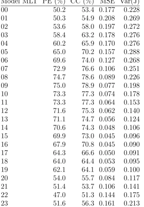
77

models would average out. The Inner Magnetosphere Particle Transport and Acceleration

78

Model (IMPTAM) [Ganushkina et al., 2013, 2014, 2015] can provided a nowcast of the

79

short time scale variations using current values of geomagnetic indices [Ganushkina et al.,

80

2015]. An empirical model of the 1 eV to 40 keV has been developed by [Denton et al.,

81

2016] as a function of local time, energy, and the strength of the solar wind electric field.

The aim of this study is to develop a reliable model that is able to forecast the short

83

spatiotemporal variations of the 40 keV electron fluxes. The NARMAX methodology used

84

to deduce the models is described in detail in Section 2, while the instrumentation and

85

data are discussed in Section 3. In Section 4.1, the data are truncated every 1 hour MLT

86

and 24 models are developed at each MLT. The performance and details of the models

87

are discussed in Section 5 and the conclusions from this study are presented in Section 6.

88

2. NARMAX methodology

NARMAX is a system identification methodology [Leontaritis and Billings, 1985a, b]

89

and was initially developed in the field of system science. In control theory, an

applica-90

tion of system science, a mathematical model of the system is needed in order to build a

91

robust controller. However, with complex engineering systems, the derivation of such a

92

mathematical model from first principles often leads to assumption which are not valid

93

and, hence, a poor controller. System identification aims to automatically derive a

math-94

ematical model that governs the system’s dynamics from input-output data. NARMAX

95

is able to deduce models for a wide range of nonlinear systems and was originally applied

96

to complex engineering systems [Billings, 2013]. The potential of the methodology to

97

develop nonlinear models from data has since been utilised by a diverse range of

scien-98

tific fields. It has been used in analyzing the adaptive changes in the photoreceptors of

99

Drosophila Flies [Friederich et al., 2009], modelling the tide at the Venice Lagoon [Wei

100

and Billings, 2006], the dynamics of Synthetic bioparts [Krishnanathan et al., 2012], and

101

the Belousov-Zhabotinsky chemical reaction [Zhao et al., 2007]. In geospace the method

102

was first used to model the Dst index and analyze the dynamics in the frequency domain

103

also been developed, using single inputs [Zhu et al., 2006], multiple inputs [Zhu et al.,

105

2007], and wavelets [Wei et al., 2004]. Boynton et al. [2011b] utilized the NARMAX

106

model structure detection methodology to identify a solar wind coupling function for

geo-107

magnetic storms, which was derived from first principles byBalikhin et al.[2010] and then

108

employed as an input to model the Dst index [Boynton et al., 2011a]. The method of using

109

the physical interpretability of the NARMAX model structure detection has since been

110

used in many other studies to identify relationships between the solar wind and various

111

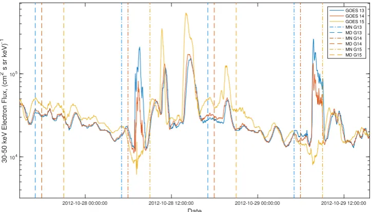
aspects of the magnetosphere. Examples include studies of SYM-H index Beharrell and

112

Honary [2016], proton fluxes at GEO [Boynton et al., 2013c], the electron fluxes [Balikhin

113

et al., 2011; Boynton et al., 2013b], and electron flux dropouts at GEO [Boynton et al.,

114

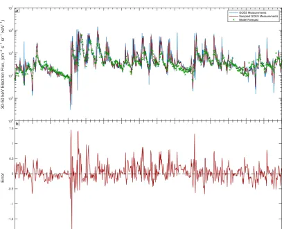
2016b] and at the GPS orbit [Boynton et al., 2017].

115

A Multi-Input Single-Output (MISO) NARMAX model was used in this study to model

116

the electron fluxes. This is represented by

117

ˆ

y(t) = F[y(t₋1), ..., y(t₋ny),

u1(t−1), ..., u1(t−nu₁), ...,

um(t−1), ..., um(t−num), ...,

e(t₋1), ..., e(t₋ne)] (1)

where an estimate of the output ˆy at time t is a nonlinear function F of past outputs

118

y, inputs u, and residual, e = y₋yˆ. m is the number of system inputs and ny, nu1,...,

119

num, ne are the maximum time lags for the output, each of the m inputs, and the error,

120

respectively.

For this study, the nonlinear function F was chosen to be a nonlinear polynomial.

122

When this polynomial is expanded there will be many monomials, most of which have no

123

influence on the system and keeping them would most likely lead to an overfit model. To

124

overcome this problem,Billings et al.[1988] developed the Forward Regression Orthogonal

125

Least Squares (FROLS) algorithm, which detects a small model structure from the larger

126

polynomial and estimates the coefficients for each of the detected monomials. The model

127

structure is detected using the Error Reduction Ratio (ERR), which indicates the influence

128

that a monomial has on the output variance. This study employs the Iterative Orthogonal

129

Forward Regression (IOFR) algorithm, which is a variant of the original FROLS. This is

130

more likely to detect the optimal model when the data is oversampled [Guo et al., 2014].

131

A more detailed description of the NARMAX methodology is described byBillings [2013]

132

orBoynton et al. [2018].

133

3. Instruments and data

The data used in this study are from the third generation GOES MAGnetospheric

Elec-134

tron Detector (MAGED) [Hanser, 2011]. The data for these instruments can be accessed

135

from http://www.ngdc.noaa.gov/stp/satellite/goes/dataaccess.html. The MAGED has 9

136

telescopes covering a range of different directions and measures the differential electron

137

fluxes in 5 energy channels: 40 keV, 75 keV, 150 keV, 275 keV and 475 keV [Hanser,

138

2011]. The time period used to derive and test the models was from 1 January 2011 to

139

13 December 2017. Three GOES spacecraft have carried this instrument, GOES 13, 14

140

and 15. These spacecraft were situated at GEO at various longitudes over North America

141

and were in operation at different times during this period.

The following MAGED data have been removed from this study due to anomalies:

143

GOES 13 on telescope 6 throughout this period; GOES 14 between 30 March 2010 and

144

2 May 2010 on telescopes 2, 5, and 8; and GOES 15 between 25 November 2017 and 31

145

December 2017 on telescope 1.

146

Solar wind data were used as input data for training and testing the models. The

1-147

minute solar wind velocity, density and Geocentric Solar Magnetospheric (GSM) IMF data

148

were obtained from the OMNI website (http://omniweb.gsfc.nasa.gov/ow min.html).

149

4. Individually binned MLT models

The method of choice of applying system identification to spatially varying systems

150

with different physics occurring in different locations is often to bin the data into different

151

spatial bins and then develop an individual model for each of the spatial bins. This

152

raises two questions: What should be the size of the spatial bin? And what should be

153

the temporal resolution of the data? With most system science applications to geospace

154

the temporal resolution is usually the resolution of the output, e.g., the Dst index has a

155

resolution of 1 hour and is modelled with a 1 hour resolution [Klimas et al., 1996]. The

156

temporal sampling frequency should be fast enough to extract the desired information

157

from the signal. Shannon’s theorem states that if the desired information has a frequency

158

fc then to recover the desired information a sampling frequency of at least 2fc is required.

159

Oversampling is not beneficial for system science modelling as the model will require the

160

inclusion of more lags, which will overcomplicate the model and increases the computation

161

time. The same is true for sampling the spatial frequency. Therefore, we need to know the

162

spatial and temporal frequency of the high flux variations of keV electrons. The electron

163

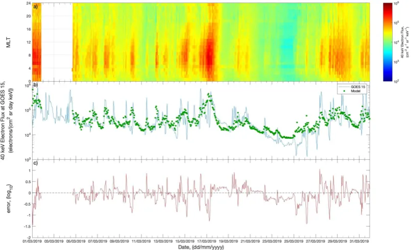
losses are due to either precipitation to the atmosphere from pitch angle scattering or

magnetopause shadowing with radial diffusion. Both these mechanisms should occur at

165

a wide range of MLT but take place over a short time period. Increases in electron flux

166

from radial diffusion will transpire over longer periods of time and increases from enhanced

167

convection will occur over a wide range of MLT at the same time. The mechanism that

168

leads to the high spatiotemporal frequency variations is due to the substorm associated

169

injections from the plasma sheet. The spatial and temporal scales at which injections

170

can occur are known to vary from one substorm to another [Sergeev and Tsyganenko,

171

1982; Ganushkina et al., 2013; Gabrielse et al., 2014], and further studies are required to

172

determine the azimuthal extent of the injection fronts. However, this study still requires

173

a spatiotemporal sampling frequency to deduce the electron flux model.

174

Figure 1 shows the 40 keV electron flux from the MAGED onboard GOES 13 (blue),

175

14 (orange) and 15 (yellow) from 27 October 2012 to 29 October 2012 and when each

176

of the spacecraft is at midday (GOES 13 blue dashed, 14 orange dashed, and 15

-177

yellow dashed) and midnight (GOES 13 - blue dot dashed, 14 - orange dot dashed, and

178

15 - yellow dot dashed). During this period, GOES 13 is 1 hour MLT ahead of GOES 14

179

and 4 hours MLT ahead of GOES 15. Up until 06 UTC on 28 October 2012, all three

180

measurements follow the same trend, with GOES 13 and 14 recording almost exactly

181

the same values and GOES 15 having a small offset. GOES 13 and 14 then observe an

182

increase of electron fluxes of approximately one order of magnitude at a post midnight

183

MLT that lasted 2 hours in time, which is not measured by GOES 15 at the pre midnight

184

MLT. This spatiotemporally localized bump in the electron flux time series is most likely

185

caused by an injection of energetic electrons from the plasma sheet. There are then a

186

series of peaks in the electron fluxes observed by all three spacecraft with GOES 13 and

14 again observing almost exactly the same values and GOES 15 having an offset. Then

188

another bump in the fluxes probably caused by an injection was observed by GOES 13

189

and 14 but not GOES 15. This increase lasted _∼ 2 hours and was observed by GOES

190

13 from 2.2 to 4.3 MLT and by GOES 14 from 1.3 to 3.4 MLT, while at the same time

191

GOES 15 moved from 22.2 to 0.3 MLT. These two potential injection structures both had

192

a temporal length of ∼2 hours and a spatial width larger than 1 hour MLT, but did not

193

extend 4 hours MLT back from GOES 13 to GOES 15. Inspecting longer periods of data

194

in which all three spacecraft are in operation does show structures with narrower temporal

195

widths but a structure observed by the middle spacecraft is almost always observed by

196

one of the other two spacecraft. Therefore, a sampling of 1 hour MLT and 1 hour time

197

was selected as a good compromise between sampling the majority of high spatiotemporal

198

frequency injections and model complexity since a higher resolution will lead to more

199

temporal lags. Electron flux enhancements through convection and radial diffusion will

200

both be oversampled in space, since convection will occur simultaneously over a broad

201

range of MLT and radial diffusion will take place at all MLT simultaneously.

202

4.1. Spatiotemporally sampled 40 keV electron flux model

The GOES 13, 14 and 15 40 keV electron flux data from the MAGED were sampled at

203

1 hour time resolution and at 1 hour MLT, smoothing over 12 minutes MLT around each

204

hour MLT, and averaging over the 9 telescopes from each spacecraft with pitch angles

205

between 20◦ _{and 160}◦ _{(excluding the errors mentioned in Section 3). This resulted in}

206

24 time series datasets for each MLT, which were then individually modelled using the

207

NARMAX methodology described in Section 2. Here, the time series of the electron flux at

208

one of the 24 MLTs is the output data,J(M LT, t). Most of the points in each of the time

series datasets were empty since for the majority of the time there will be no spacecraft

210

in the MLT bin. The input data employed were the solar wind velocity v(t), density

211

n(t), square root of the pressure √p(t), and the IMF factor Bf(t) = BT(t) sin6(θ(t)/2)

212

(whereBT(t) =

p

By(t)2+Bz(t)2andθ = tan−1(By(t)/Bz(t))) deduced byBoynton et al.

213

[2011b] and Balikhin et al. [2010]. The output lags were selected as the value 24 hours

214

previous. This is the most consistent data point that will be available, since any other

215

output lag will most likely be empty in the constructed time series dataset. The input

216

time lags were selected as 1, 3, 5,..., 23 hours as it has been shown that 10 to 100 keV

217

electrons have short response times with solar wind variations compared to MeV electrons

218

[Li et al., 2005; Boynton et al., 2013b]. The noise terms were not included in the model

219

because these data were sparse. This reduces the NARMAX model to the following NARX

220

model:

221

ˆ

J(M LT, t) = F[J(M LT, t−24),

v(t₋1), v(t₋3), ..., v(t₋23),

n(t₋1), n(t₋3), ..., n(t₋23),

√

p(t−1),√p(t−3), ...,√p(t−23),

Bf(t−1), Bf(t−3), ..., Bf(t−23)] (2)

The nonlinear function F was chosen to be a third degree polynomial, thus, the model

222

can include linear monomials of the lagged inputs and outputs as well as cross coupled

223

combinations of the lagged inputs and outputs.

224

The IOFR algorithm was run for each of the 24 datasets using the same NARX model

225

on data from 00:00 UTC 1 January 2011 to 23:00 UTC 28 February 2013. These models

were then assessed statistically on data from 1 March 2013 to 31 December 2017 using the

227

Prediction Efficiency (PE), Eq. (3), Correlation Coefficient (CC), Eq. (4), Mean Square

228

Error (MSE), and the variance of the observed flux, which are commonly used to assess

229

models [Temerin and Li, 2006;Li, 2004;Boynton et al., 2011a;Wei et al., 2004;Boynton

230

et al., 2015; Rastatter et al., 2013]. The equations for PE and CC are:

231

EP E =

      1− N X t=1

(y(t)₋yˆ(t))2

N

X

t=1

(y(t)₋y¯)2       100% (3)

ρyyˆ =

N

X

t=1

(y(t)−y¯) ˆy(t)−y¯ˆ

v u u t N X t=1

(y(t)₋y¯)2

N

X

t=1

h

ˆ

y(t)₋y¯ˆ2i

100% (4)

EM SE =

N

X

t=1

(y(t)−yˆ(t))2 (5)

Here, EP E is the PE, ρ is the CC, EM SE is the MSE, y(t) is the measured output at

232

time t, ˆy is the estimated output from the model, N is the length of the data and the

233

bar signifies the average. The model performance statistics of each of these models are

234

displayed in Table 1. The PE for each model varies by 47% and 75% while the CC varies

235

between 51.3% and 78.9%. The highest PE and CC occur at 09 MLT and decreases to the

236

lowest PE and CC at 22 MLT. The MSE and variance have a similar sinusoidal pattern

237

with both having a minimum at 16 MLT of 0.045 and 0.090 respectively and the MSE

238

having a maximum at 01 MLT of 0.208, while the maximum of the variance is 0.288 at

239

05 MLT.

Figure 2 shows the model estimate of the 40 keV electron fluxes from 1 November 2017

241

to 30 November 2017 for different MLT. During this period, the model forecasts a number

242

of enhancements that are most intense at dawn MLTs and are lowest at evening MLTs.

243

Even though all the estimates at each MLT are from a different model, the structure of the

244

plots is consistent. A surface plot of the forecast is good for showing the evolution of the

245

fluxes but will be not be able to illustrate the performance of the model compared to the

246

observed fluxes, since, at each point in time, there will only be a few MLT measurements.

247

Figure 3 (a) shows a comparison of the model with GOES 13 measurements for the same

248

1 November 2017 to 30 November 2017 period displayed in Figure 2. The 1 minute GOES

249

13 data is presented in blue, the spatiotemporal sampled GOES data in red and the

250

model forecast at the GOES 13 location shown in green. Panel (b) displays the error

251

between the sampled GOES 13 40 keV electron flux and the model forecast at the GOES

252

13 location. The model forecast is shown to follow the enhancements and decreases of

253

the measured electron flux data with a MSE of 0.083 log10 for the displayed period. The

254

model is able to forecast the large variations, for example, the decrease and the increase

255

on 3 November 2017, but struggles to reproduce the higher frequency variations. A video

256

of the variations in electron flux at different MLT for the period in Figures 2 and 3 are in

257

the supplementary material.

258

5. Discussion

One advantage of NARMAX methodologies over neural network machine learning

tech-259

niques, other than its resilience to overfitting, is that the models are physically

inter-260

pretable. The resulting models from the NARMAX algorithm are polynomials consisting

261

were selected for the model, it is possible to gain some understanding into the underlying

263

physical processes of the system [Balikhin et al., 2010; Boynton et al., 2011b; Balikhin

264

et al., 2012; Boynton et al., 2013b; Billings, 2013]. The model for the 01 MLT 40 keV

265

electron fluxes is

266

ˆ

J(01M LT, t) = 3.21_×10−4

Bf(t−1)v(t−1) + 2.57 + 1.78×10−3v(t−5)

+4.02_×10−2_B

f(t−5)−4.51×10−3Bf2(t−1)

+1.07×10−2J2(01M LT, t−24)−1.46×10−1p(t−3)

+5.91×10−2Bf(t−21) + 4.72×10−1√p(t−3) + 1.47×10−3v(t−17)

−4.69×10−3Bf(t−20)Bf(t−21)−3.74×10−2Bf(t−1)√p(t−1)

+7.35_×10−2_B

f(t−13)−3.41×10−2Bf(t−13)√p(t−14)

−5.87×10−3Bf2(t−7) + 5.16×10−

2

Bf(t−7)

−1.34×10−6v(t−8)v(t−9) (6)

One interesting point about the models deduced by the algorithm using the initial NARX

267

model structure in Eq. (2) is that only the 01 MLT, 04 MLT, and 18 MLT models

268

out of the 24 models included the autoregressive J(M LT, t− 24) term out of the 24

269

models. The autoregressive monomials in each of the three NARX models only have a

270

small contribution to the variance of the output, indicated by the small ERR. The other

271

models, with no past output terms and only consisting of exogenous terms, are known as

272

Volterra Series models. The lack of autoregressive terms and the small ERR contribution

273

when they are selected in the model means that the hourly MLT electron flux changes

274

significantly from their value 24 hours ago.

The variable that is selected in all the models, and appears as a factor of the monomial

276

that has the highest ERR in each of the models, is the IMF factor Bf. The monomial

277

with the highest ERR controls most of the output variance. The solar wind velocity is

278

the second most selected variable and it is in all the models in either the first or second

279

highest ERR monomial, often coupled withBf. The square root of the solar wind pressure

280

is chosen by the algorithm in 23 of the models (not the 23 MLT model) and the solar

281

wind density is only selected in 14 of the models but both are rarely selected in the top

282

five terms in order of ERR (three times for both pressure and density) and, thus, only

283

have a small contribution to the variance of the output.

284

The IMF factorBf was automatically identified in a solar wind-magnetosphere coupling

285

function by using the NARMAX FROLS methodology and then derived analytically from

286

first principles by Balikhin et al. [2010]. This derivation is based on the geometry of

287

the dayside magnetosphere reconnection with the solar wind. Therefore, the fact that the

288

models attribute most of the variation of the electron fluxes to the IMF factor implies that

289

the reconnection is the most important process. On the surface, this is in contrast to the

290

higher energies where solar wind velocity [Paulikas and Blake, 1979] or density [Balikhin

291

et al., 2011] was found to have the most influence. However, these studies investigated

292

the daily averages of electron fluxes and solar wind, which will average out the turning

293

of the IMF southward over the day, since these time scales are quite short (∼ 1 hour).

294

With the increased temporal resolution the turning of the IMF southward will not be

295

averaged out and and will have more influence. This averaging out over the timescales of

296

the IMF variations is also true for the study by Boynton et al. [2013b] where they also

297

found that southward IMF only had a small influence on the daily averaged 10 to 100 keV

electron fluxes. For example, if there is a high velocity solar wind event taking place over

299

several days and there are several periods of time when the IMF is southward for an hour,

300

the IMF may average out to be insignificant, while the velocity remains high. Therefore,

301

choosing a different time resolution may change the importance of the parameters.

302

The performance of the different electron flux models show a pattern with the MLT,

303

with the highest performance in terms of CC and PE in the late morning and the lowest

304

performance just before midnight. The lower performance just before midnight could

305

be due to the model not performing very well at forecasting the higher spatiotemporal

306

frequency injections that occur in this region. The MSE also exhibits a pattern with MLT

307

but it is shifted compared to PE and CC, with the highest MSE at 01 MLT and the lowest

308

at 15 and 16 MLT. The shift between PE and CC variation with MLT and the MSE MLT

309

variation is mainly due to the difference in the electron flux variance at each MLT, since

310

both PE and CC are normalized by the variance of the measured electron fluxes.

311

The highest performance in terms of PE and CC occur at dayside MLTs, where the

312

increases in the fluxes will mostly be due to convection or radial diffusion and are unlikely

313

to be caused by substorm particle injections. From Figure 3, the model estimates the

314

majority of the structures that last over half a day but a magnified figure would show more

315

detail. Figure 4 displays two magnified sections of Figure 3, panel (a) from 10 November

316

2017 to 12 November 2017, and panel (b) from 20 November 2017 to 22 November 2017.

317

The Figures show that the model follows the general trend of the measured GOES 13

318

data during this period. There is a sharp peak in the 1 minute GOES 13 measurements

319

(blue) on 10 November 2017 at 0400 UTC, which is averaged out in the sampled GOES

320

measurement (red), however, the model (green) does show an increase. Overall, the model

underperforms in forecasting the high spatial and temporal frequency variations, such as

322

the three peaks between 0600-1800 UTC on 11 November 2017, but follows the slower

323

variations. An increased temporal resolution of 30 minutes may help in identifying the

324

fast substorm associated injections. The inputs to the model are measured at L1 and using

325

a 1 hour time lag in the model, which may lead to changes in the solar wind occurring

326

inside the hour. For example, a fast flow of solar wind can transit from L1 to the bow

327

shock in under 30 minutes, which will cause a change in the magnetosphere that the 1

328

hour lags in the model will be unable to take into account. Therefore, in the training of

329

the model, these changes in solar wind cannot be identified as drivers of the changes in

330

the electron fluxes. However, a consequence of including shorter lags in the model will be

331

to reduce the forecast horizon of the model. Also, the averaging of the solar wind over the

332

hour, particularly the fast turning of the solar wind southward, may nullify the drivers

333

of the substorm, therefore, it will not be identified in the model. This problem could be

334

solved by including the maximum of the value of the solar wind parameters as inputs as

335

well as the average value, however, this would increase the computational complexity of

336

identifying the model due to an increased amount of monomials to search through.

337

Another option to spatially model the electron fluxes is to employ MLT as an input

338

into the model, rather than sampling the data in space and developing a separate model

339

for each spatial bin. However, this approach was not selected because at different MLTs

340

there should be different dynamics, and it would be better to isolate the individual physical

341

processes in the different models corresponding to each region.

342

A model of the 40 keV electron fluxes through all MLTs at geostationary orbit is not only

343

useful to satellite operators, who would be able to have a greater situational awareness of

the environment and be able to apply any mitigation procedures to help protect their space

345

based assets. The model could also be used as an outer boundary condition to physics

346

based radiation belt models such as the Versatile Electron Radiation Belt (VERB) model

347

[Subbotin et al., 2011], Comprehensive Inner Magnetosphere-Ionosphere (CIMI) model

348

[Fok et al., 2014] or IMPTAM [Ganushkina et al., 2015].

349

The models developed in this study have been implemented to run in real time. A figure

350

of the real time output of this model is shown in Figure 5, which shows the model output

351

across all MLT in panel (a), the model output at the location of GOES 15 vs GOES 15

352

data, and (c) the error between the measured and model for March 2019. The model

353

performance for this period were a PE of 48.5% and a CC of 66.3%. The data gap at the

354

start of the month is due to a missing solar wind inputs, which were not available from

355

NOAA Space Weather Prediction Center (SWPC) at the time the forecast was made.

356

6. Conclusions

A data based spatiotemporal model has been developed for the 40 keV electron fluxes

357

at GEO. This model is comprised of 24 individual NARX models of the form shown

358

in Equation (2), where the output of each model is the electron fluxes for that region

359

of space in MLT at GEO. When the 24 models are conjugated together into the final

360

model, they give a forecast of the spatiotemporal evolution of the 40 keV electron fluxes

361

at GEO. At this energy, the electron fluxes can vary significantly over a narrow range of

362

MLTs due to substorm associated injections making it very challenging to model. The

363

development of a data based model using system science techniques is complicated by

364

the sparse availability of the electron fluxes at different MLT. This problem was solved

365

by binning the data from GOES 13, 14, and 15 by MLT and then deducing a separate

model for each bin then conjugating these to produce one spatiotemporal forecast. The

367

performance of this forecast was then assessed on a period from 1 March 2013 to 31

368

December 2017 where the PE varied between 47% and 75% and the CC varied between

369

51.3% and 78.9% at different MLTs.

370

The models developed in this study will be implemented online at the University of

371

Sheffield Space Weather Website (http://www.ssg.group.shef.ac.uk/USSW2/UOSSW.html)

372

to provide a real time forecast of the GEO 40 keV electron fluxes through all MLTs. This

373

will allow both satellite operators and scientists to have access to the outputs of the

374

models, which will also be archived.

375

Acknowledgments. The MAGED data can be accessed from

376

http://www.ngdc.noaa.gov/stp/satellite/goes/dataaccess.html. The solar wind data and

377

geomagnetic indices data were from the OMNI website (http://omniweb.gsfc.nasa.gov/ow min.html).

378

The real time data were from the NOAA SWPC. The work was performed within the

379

project Rad-Sat and has received financial support from the UK NERC under grant

380

NE/P017061/1.

381

References

Bailey, D. K., Some quantitative aspects of electron precipitation in and near the auroral

382

zone, Rev. Geophys., 6(3), 289–346, 1968.

383

Baker, D., R. Belian, P. Higbie, R. Klebesadel, and J. Blake, Deep dielectric charging

384

effects due to high-energy electrons in earth’s outer magnetosphere, Journal of

Electro-385

statics,20(1), 3–19, 1987.

Baker, D. N., R. L. McPherron, T. E. Cayton, and R. W. Klebesadel, Linear prediction

387

filter analysis of relativistic electron properties at 6.6 re, J. Geophys. Res., 95(A9),

388

15,133–15,140, 1990.

389

Balikhin, M. A., O. M. Boaghe, S. A. Billings, and H. S. C. K. Alleyne, Terrestrial

390

magnetosphere as a nonlinear resonator, Geophys. Res. Lett.,28(6), 1123–1126, 2001.

391

Balikhin, M. A., R. J. Boynton, S. A. Billings, M. Gedalin, N. Ganushkina, D. Coca, and

392

H. Wei, Data based quest for solar wind-magnetosphere coupling function, Geophys.

393

Res. Lett., 37(24), L24,107, 2010.

394

Balikhin, M. A., R. J. Boynton, S. N. Walker, J. E. Borovsky, S. A. Billings, and H. L.

395

Wei, Using the narmax approach to model the evolution of energetic electrons fluxes at

396

geostationary orbit, Geophys. Res. Lett., 38(18), L18,105, 2011.

397

Balikhin, M. A., M. Gedalin, G. D. Reeves, R. J. Boynton, and S. A. Billings, Time scaling

398

of the electron flux increase at geo: The local energy diffusion model vs observations,

399

J. Geophys. Res.,117(A10), A10,208–, 2012.

400

Balikhin, M. A., J. V. Rodriguez, R. J. Boynton, S. N. Walker, H. Aryan, D. G. Sibeck,

401

and S. A. Billings, Comparative analysis of noaa refm and snb3geo tools for the forecast

402

of the fluxes of high-energy electrons at geo, Space Weather, 14(1), 2015SW001,303–,

403

2016.

404

Beharrell, M. J., and F. Honary, Decoding solar wind-magnetosphere coupling, Space

405

Weather, n/a, 2016SW001,467–, 2016.

406

Billings, S., M. Korenberg, and S. Chen, Identification of non-linear output affine systems

407

using an orthogonal least-squares algorithm., Int. J. of Systems Sci., 19, 1559–1568,

408

1988.

Billings, S. A., Nonlinear System Identification: NARMAX Methods in the Time,

Fre-410

quency, and Spatio-Temporal Domains, Wiley, 2013.

411

Boaghe, O. M., M. A. Balikhin, S. A. Billings, and H. Alleyne, Identification of nonlinear

412

processes in the magnetospheric dynamics and forecasting of dst index, J. Geophys.

413

Res.,106(A12), 30,047–30,066, 2001.

414

Bortnik, J., R. M. Thorne, T. P. O’Brien, J. C. Green, R. J. Strangeway, Y. Y. Shprits,

415

and D. N. Baker, Observation of two distinct, rapid loss mechanisms during the 20

416

november 2003 radiation belt dropout event, J. Geophys. Res., 111(A12), A12,216–,

417

2006.

418

Boynton, R., M. Balikhin, H.-L. Wei, and Z.-Q. Lang, Machine Learning Techniques

419

for Space Weather, chap. Applications of NARMAX in Space Weather, pp. 203–237,

420

Elsevier, 2018.

421

Boynton, R. J., M. A. Balikhin, S. A. Billings, A. S. Sharma, and O. A. Amariutei, Data

422

derived narmax dst model, Annales Geophysicae, 29(6), 965–971,

doi:10.5194/angeo-423

29-965-2011, 2011a.

424

Boynton, R. J., M. A. Balikhin, S. A. Billings, H. L. Wei, and N. Ganushkina, Using the

425

narmax ols-err algorithm to obtain the most influential coupling functions that affect

426

the evolution of the magnetosphere, J. Geophys. Res., 116(A5), A05,218, 2011b.

427

Boynton, R. J., M. A. Balikhin, S. A. Billings, and O. A. Amariutei, Application of

428

nonlinear autoregressive moving average exogenous input models to geospace: advances

429

in understanding and space weather forecasts,Ann. Geophys.,31(9), 1579–1589, 2013a.

430

Boynton, R. J., M. A. Balikhin, S. A. Billings, G. D. Reeves, N. Ganushkina, M. Gedalin,

431

O. A. Amariutei, J. E. Borovsky, and S. N. Walker, The analysis of electron fluxes at

geosynchronous orbit employing a narmax approach, J. Geophys. Res. Space Physics,

433

118(4), 1500–1513, 2013b.

434

Boynton, R. J., S. A. Billings, O. A. Amariutei, and I. Moiseenko, The coupling between

435

the solar wind and proton fluxes at geo, Ann. Geophys.,31(10), 1631–1636, 2013c.

436

Boynton, R. J., M. A. Balikhin, and S. A. Billings, Online narmax model for electron

437

fluxes at geo, Ann. Geophys., 33(3), 405–411, 2015.

438

Boynton, R. J., M. A. Balikhin, D. G. Sibeck, S. N. Walker, S. A. Billings, and N.

Ganushk-439

ina, Electron flux models for different energies at geostationary orbit, Space Weather,

440

14(10), 2016SW001,506–, 2016a.

441

Boynton, R. J., D. Mourenas, and M. A. Balikhin, Electron flux dropouts at geostationary

442

earth orbit: Occurrences, magnitudes, and main driving factors,J. Geophys. Res. Space

443

Physics, 121(9), 2016JA022,916–, 2016b.

444

Boynton, R. J., D. Mourenas, and M. A. Balikhin, Electron flux dropouts at l 4.2 from

445

global positioning system satellites: Occurrences, magnitudes, and main driving factors,

446

J. Geophys. Res. Space Physics, 122(11), 11,428–11,441, doi:10.1002/2017ja024523,

447

2017.

448

Denton, M. H., M. G. Henderson, V. K. Jordanova, M. F. Thomsen, J. E. Borovsky,

449

J. Woodroffe, D. P. Hartley, and D. Pitchford, An improved empirical model of electron

450

and ion fluxes at geosynchronous orbit based on upstream solar wind conditions, Space

451

Weather, 14(7), 511–523, doi:10.1002/2016sw001409, 2016.

452

Ferguson, D. C., Chapter 15 - extreme space weather spacecraft surface charging and

453

arcing effects, in Extreme Events in Geospace, edited by N. Buzulukova, pp. 401–418,

454

Elsevier, 2018.

Fok, M. C., N. Y. Buzulukova, S. H. Chen, A. Glocer, T. Nagai, P. Valek, and J. D.

456

Perez, The comprehensive inner magnetosphere-ionosphere model, J. Geophys. Res.

457

Space Physics, 119(9), 7522–7540, doi:10.1002/2014JA020239, 2014.

458

Freeman, J. W., T. P. O’Brien, A. A. Chan, and R. A. Wolf, Energetic electrons at

459

geostationary orbit during the november 3-4, 1993 storm: Spatial/temporal morphology,

460

characterization by a power law spectrum and, representation by an artificial neural

461

network, J. Geophys. Res., 103(A11), 26,251–26,260, 1998.

462

Friedel, R., G. Reeves, and T. Obara, Relativistic electron dynamics in the inner

mag-463

netosphere - a review, Journal of Atmospheric and Solar-Terrestrial Physics, 64(2),

464

265–282, 2002.

465

Friederich, U., D. Coca, S. A. Billings, and M. Juusola, Data modelling for analysis of

466

adaptive changes in fly photoreceptors, Neural Information Processing, PT 1,

Proceed-467

ings,5863, 34–38, 2009.

468

Gabrielse, C., V. Angelopoulos, A. Runov, and D. L. Turner, Statistical characteristics

469

of particle injections throughout the equatorial magnetotail, J. Geophys. Res. Space

470

Physics, 119(4), 2512–2535, doi:10.1002/2013ja019638, 2014.

471

Ganushkina, N. Y., O. A. Amariutei, Y. Y. Shprits, and M. W. Liemohn, Transport of the

472

plasma sheet electrons to the geostationary distances, J. Geophys. Res. Space Physics,

473

118(1), 82–98, 2013.

474

Ganushkina, N. Y., M. W. Liemohn, O. A. Amariutei, and D. Pitchford, Low-energy

475

electrons (5-50 kev) in the inner magnetosphere,J. Geophys. Res. Space Physics,119(1),

476

246–259, 2014.

Ganushkina, N. Y., O. A. Amariutei, D. Welling, and D. Heynderickx, Nowcast

478

model for low-energy electrons in the inner magnetosphere, Space Weather, 13(1),

479

2014SW001,098–, 2015.

480

Gubby, R., and J. Evans, Space environment effects and satellite design, Journal of

At-481

mospheric and Solar-Terrestrial Physics,64(16), 1723–1733, 2002.

482

Guo, Y., L. Guo, S. Billings, and H.-L. Wei, An iterative orthogonal forward

re-483

gression algorithm, International Journal of Systems Science, 46(5), 776–789, doi:

484

10.1080/00207721.2014.981237, 2014.

485

Hanser, F. A., Eps/hepad calibration and data handbook,Tech. rep., Tech. Rep.

GOESN-486

ENG-048D, Assurance Technol. Corp., Carlisle, Mass., 2011.

487

Horne, R. B., S. A. Glauert, N. P. Meredith, D. Boscher, V. Maget, D. Heynderickx, and

488

D. Pitchford, Space weather impacts on satellites and forecasting the earth’s electron

489

radiation belts with spacecast, Space Weather, 11, 1–18, 2013a.

490

Horne, R. B., S. A. Glauert, N. P. Meredith, H. Koskinen, R. Vainio, A. Afanasiev,

491

N. Y. Ganushkina, O. A. Amariutei, D. Boscher, A. Sicard, V. Maget, S. Poedts,

492

C. Jacobs, B. Sanahuja, A. Aran, D. Heynderickx, and D. Pitchford, Forecasting the

493

earth’s radiation belts and modelling solar energetic particle events: Recent results from

494

spacecast, J. Space Weather Space Clim., 3, A20, 2013b.

495

Kim, H.-J., and A. A. Chan, Fully adiabatic changes in storm time relativistic electron

496

fluxes, J. Geophys. Res., 102(A10), 22,107–22,116, 1997.

497

Klimas, A. J., D. Vassiliadis, D. N. Baker, and D. A. Roberts, The organized nonlinear

498

dynamics of the magnetosphere, J. Geophys. Res., 101(A6), 13,089–13,113, 1996.

Koons, H. C., and D. J. Gorney, A neural network model of the relativistic electron flux

500

at geosynchronous orbit, J. Geophys. Res., 96(A4), 5549–5556, 1991.

501

Krishnanathan, K., S. R. Anderson, S. A. Billings, and V. Kadirkamanathan, A

data-502

driven framework for identifying nonlinear dynamic models of genetic parts,ACS Synth.

503

Biol.,1(8), 375–384, doi:10.1021/sb300009t, 2012.

504

Leontaritis, I. J., and S. A. Billings, Input-output parametric models for non-linear

sys-505

tems part i: Deterministic non-linear systems., Int. J. Control,41 (2), 303–328, 1985a.

506

Leontaritis, I. J., and S. A. Billings, Input-output parametric models for non-linear

sys-507

tems part ii: Stochastic nonlinear systems, Int. J. Control, 41 (2), 329–344, 1985b.

508

Li, X., Variations of 0.7-6.0 mev electrons at geosynchronous orbit as a function of solar

509

wind, Space Weather, 2(3), S03,006, 2004.

510

Li, X., D. N. Baker, M. Temerin, G. Reeves, R. Friedel, and C. Shen, Energetic electrons,

511

50 kev to 6 mev, at geosynchronous orbit: Their responses to solar wind variations,

512

Space Weather,3(4), S04,001–, 2005.

513

Ling, A. G., G. P. Ginet, R. V. Hilmer, and K. L. Perry, A neural network-based

geosyn-514

chronous relativistic electron flux forecasting model, Space Weather, 8(9), S09,003–,

515

2010.

516

Lohmeyer, W., and K. Cahoy, Space weather radiation effects on geostationary satellite

517

solid-state power amplifiers, Space Weather, 11(8), 476–488, 2013.

518

Lohmeyer, W., A. Carlton, F. Wong, M. Bodeau, A. Kennedy, and K. Cahoy, Response

519

of geostationary communications satellite solid-state power amplifiers to high-energy

520

electron fluence, Space Weather, 13(5), 2014SW001,147–, 2015.

Loto’aniu, T. M., H. J. Singer, J. V. Rodriguez, J. Green, W. Denig, D. Biesecker, and

522

V. Angelopoulos, Space weather conditions during the galaxy 15 spacecraft anomaly,

523

Space Weather,13(8), 484–502, Aug. 2015.

524

Mullen, E. G., M. S. Gussenhoven, D. A. Hardy, T. A. Aggson, B. G. Ledley, and

525

E. Whipple, Scatha survey of high-level spacecraft charging in sunlight, J. Geophys.

526

Res.,91(A2), 1474–1490, 1986.

527

O’Brien, T. P., and C. L. Lemon, Reanalysis of plasma measurements at geosynchronous

528

orbit, Space Weather, 5(3), doi:10.1029/2006sw000279, 2007.

529

Olsen, R. C., A threshold effect for spacecraft charging, J. Geophys. Res., 88(A1), 493–

530

499, 1983.

531

Osthus, D., P. C. Caragea, D. Higdon, S. K. Morley, G. D. Reeves, and B. P. Weaver,

532

Dynamic linear models for forecasting of radiation belt electrons and limitations on

533

physical interpretation of predictive models, Space Weather,12(6), 426–446, 2014.

534

Paulikas, G. A., and J. B. Blake, Effects of the solar wind on magnetospheric dynamics:

535

Energetic electrons at the synchronous orbit, Quantitative Modeling of Magnetospheric

536

Processes, Geophys. Monogr. Ser.,21, 180–202, aGU, Washington, D. C., 1979.

537

Rastatter, L., M. M. Kuznetsova, A. Glocer, D. Welling, X. Meng, J. Raeder, M.

Wilt-538

berger, V. K. Jordanova, Y. Yu, S. Zaharia, R. S. Weigel, S. Sazykin, R. Boynton,

539

H. Wei, V. Eccles, W. Horton, M. L. Mays, and J. Gannon, Geospace environment

540

modeling 2008-2009 challenge: Dst index, Space Weather,11(4), 187–205, 2013.

541

Rigler, E. J., D. N. Baker, R. S. Weigel, D. Vassiliadis, and A. J. Klimas, Adaptive linear

542

prediction of radiation belt electrons using the kalman filter, Space Weather, 2(3), doi:

543

10.1029/2003sw000036, 2004.

Sarno-Smith, L. K., B. A. Larsen, R. M. Skoug, M. W. Liemohn, A. Breneman,

545

J. R. Wygant, and M. F. Thomsen, Spacecraft surface charging within

geosyn-546

chronous orbit observed by the van allen probes, Space Weather, 14(2), 151–164, doi:

547

10.1002/2015sw001345, 2016.

548

Sergeev, V., and N. Tsyganenko, Energetic particle losses and trapping boundaries as

549

deduced from calculations with a realistic magnetic field model, Planetary and Space

550

Science,30(10), 999–1006, 1982.

551

Subbotin, D. A., Y. Y. Shprits, and B. Ni, Long-term radiation belt simulation with

552

the verb 3-d code: Comparison with crres observations, J. Geophys. Res., 116(A12),

553

A12,210–, 2011.

554

Temerin, M., and X. Li, Dst model for 1995 - 2002, J. Geophys. Res., 111(A4), A04,221,

555

2006.

556

Thomsen, M. F., M. G. Henderson, and V. K. Jordanova, Statistical properties of the

557

surface-charging environment at geosynchronous orbit,Space Weather, 11(5), 237–244,

558

doi:10.1002/swe.20049, 2013.

559

Turner, D. L., Y. Shprits, M. Hartinger, and V. Angelopoulos, Explaining sudden losses

560

of outer radiation belt electrons during geomagnetic storms, Nat Phys, 8(3), 208–212,

561

2012.

562

Wei, H. L., and S. A. Billings, An efficient nonlinear cardinal b-spline model for high

563

tide forecasts at the venice lagoon,Nonlinear Processes In Geophysics, 13(5), 577–584,

564

2006.

565

Wei, H. L., S. A. Billings, and M. Balikhin, Prediction of the dst index using

multireso-566

lution wavelet models, J. Geophys. Res.,109(A7), A07,212, 2004.

Wei, H.-L., S. A. Billings, A. Surjalal Sharma, S. Wing, R. J. Boynton, and S. N. Walker,

568

Forecasting relativistic electron flux using dynamic multiple regression models,Annales

569

Geophysicae, 29(2), 415–420, doi:10.5194/angeo-29-415-2011, 2011.

570

Wrenn, G. L., D. J. Rodgers, and K. A. Ryden, A solar cycle of spacecraft anomalies due

571

to internal charging, Ann. Geophys., 20(7), 953–956, 2002.

572

Zhao, Y., S. A. Billings, and A. F. Routh, Identification of the belousov-zhabotinskii

re-573

action using cellular automata models, International Journal of Bifurcation and Chaos,

574

17(5), 1687–1701, doi:10.1142/S0218127407017999, 2007.

575

Zhu, D., S. A. Billings, M. Balikhin, S. Wing, and D. Coca, Data derived continuous time

576

model for the dst dynamics, Geophys. Res. Lett., 33(4), L04,101, 2006.

577

Zhu, D., S. A. Billings, M. A. Balikhin, S. Wing, and H. Alleyne, Multi-input data derived

578

dst model, J. Geophys. Res., 112(A6), A06,205, 2007.

Model MLT PE (%) CC (%) MSE Var(J)

00 50.2 53.4 0.177 0.228

01 50.3 54.9 0.208 0.269

02 53.6 58.0 0.197 0.272

03 58.4 63.2 0.178 0.276

04 60.2 65.9 0.170 0.276

05 65.0 70.2 0.157 0.288

06 69.6 74.0 0.127 0.268

07 72.9 76.6 0.106 0.251

08 74.7 78.6 0.089 0.226

09 75.0 78.9 0.077 0.198

10 73.3 77.3 0.074 0.178

11 73.3 77.3 0.064 0.153

12 71.6 75.3 0.062 0.140

13 71.1 74.7 0.056 0.124

14 70.6 74.3 0.048 0.106

15 69.9 73.0 0.045 0.096

16 67.9 70.8 0.045 0.090

17 64.3 66.6 0.050 0.091

18 64.0 64.4 0.053 0.095

19 62.1 64.1 0.059 0.100

20 54.0 55.7 0.084 0.117

21 51.4 53.7 0.106 0.141

22 47.0 51.3 0.144 0.175

23 51.6 56.3 0.161 0.213

Table 1. Table showing the PE, CC, MSE for each MLT model and the variance of the

2012-10-28 00:00:00 2012-10-28 12:00:00 2012-10-29 00:00:00 2012-10-29 12:00:00 Date

104 105

30-50 keV Electron Flux, (cm

2 s sr keV)

-1

GOES 13 GOES 14 GOES 15 MN G13 MD G13 MN G14 MD G14 MN G15 MD G15

Figure 1. The 40 keV electron flux observed by the MAGED onboard GOES 13 (blue), 14

(orange) and 15 (yellow) between 27 October 2012 and 29 October 2012. The figure also shows

when each of the spacecraft is at midday (GOES 13 - blue dashed, 14 - orange dashed, and 15

yellow dashed) and midnight (GOES 13 blue dot dashed, 14 orange dot dashed, and 15

-yellow dot dashed).

Figure 2. The model estimated 40 keV electron flux at all MLT from 1 November 2017 to 30

Date

102

103

104

105

106

107

30-50 keV Electron Flux, (cm

-2

s

-1 sr -1 keV

-1

)

a) _{GOES Measurements}

Sampled GOES Measurements Model Forecast

01/11/2017 03/11/2017 05/11/2017 07/11/2017 09/11/2017 11/11/2017 13/11/2017 15/11/2017 17/11/2017 19/11/2017 21/11/2017 23/11/2017 25/11/2017 27/11/2017 29/11/2017 01/12/2017

Date

-2 -1.5 -1 -0.5 0 0.5 1 1.5

Error

b)

Figure 3. (a) The 40 keV electron flux observed by the MAGED onboard GOES 13 (blue), the

sampled GOES 13 40 keV electron flux (red) and the model forecast at the GOES 13 location

for November 2017. (b) The error between the sampled GOES 13 40 keV electron flux and the

2017-11-10 00:00:00 2017-11-10 12:00:00 2017-11-11 00:00:00 2017-11-11 12:00:00 2017-11-12 00:00:00 Date

104 105 106

30-50 keV Electron Flux, (cm

-2 s

-1

sr

-1 keV

-1) a) GOES Measurements_{Sampled GOES Measurements}

Model Forecast

2017-11-20 00:00:00 2017-11-20 12:00:00 2017-11-21 00:00:00 2017-11-21 12:00:00 2017-11-22 00:00:00

Date 103

104 105 106

30-50 keV Electron Flux, (cm

-2 s

-1

sr

-1

keV

-1) b) GOES Measurements

Sampled GOES Measurements Model Forecast

Figure 4. The 40 keV electron flux observed by the MAGED onboard GOES 13 (blue), the

sampled GOES 13 40 keV electron flux (red) and the model forecast at the GOES 13 location

Figure 5. The real time output from the 40 keV electron flux model: (a) in MLT and time (b)

at the GOES 15 location (green) vs GOES 15 data (blue), and (c) the error between the sampled