Trends in building energy modelling and simulation
J A Clarke
Energy Systems Research Unit
University of Strathclyde
Abstract
This paper summarises the state-of-the-art in integrated building performance assessment and describes current development trends aimed at ensuring the technology keeps pace with evolving user demand.
Keywords: integrated building performance assessment, capabilities, trends.
Introduction
Because the built environment consumes a large portion of total delivered energy and is responsible for much of the avoidable CO2
emissions, many initiatives are focused on this sector. However, buildings are complex, and in the absence of a means to predict the performance benefit of proposed measures, many of these initiatives will fail. Modelling methods, when embedded within the design process, allow practitioners to pursue new designs and refurbishments that conform to legislative requirements; provide requisite levels of comfort and indoor air quality; integrate new and renewable energy technologies; and mitigate emissions.
Because the energy domain is complex, conflicting viewpoints abound, proffered solutions are sometimes polarised and consensus is difficult to attain. One way to address these difficulties is to give practitioners the means to assess the overall performance of design options prior to construction. This paper reports current development trends relating to a technology that may be used to this end – integrated building performance modelling.
Building Simulation Practice
It is widely accepted that integrated modelling defines a new best practice approach (CIBSE 1998) to building design because it allows designers to link energy, the environment and health. In use, the approach requires the gradual evolution of a design description, with performance outputs becoming available at discrete stages as summarised in Table 1. The design team is then free to terminate model evolution when objectives have been met.
Consider the scenario of Figure 1, which highlights the integrated appraisal approach and, by implication, indicates a possible future design practice. This scenario is based on the ESP-r system (Clarke 2001) when its data model is cumulatively refined as described in Table 1.
a1 A Project Manager (Hand 1998) gives access to support databases, model definition tools, a simulation engine, and performance assessment tools. Its role is to co-ordinate problem definition and pass data models between applications as a problem is incrementally evolved.
b1 Projects commence by making ready system databases. These typically include hygro-thermal, embodied energy and optical properties for constructions, typical occupancy profiles, pressure coefficient sets, plant components, and climate collections representing different locations and weather severity.
c1 Embedded within such databases is knowledge that supports design conceptualisation. For example, the construction elements database contains derived properties from which behaviour may be deduced (e.g. thermal diffusivity to characterise a construction’s rate of response or thermal transmittance to characterise its rate of heat loss).
d1
It is common to commence problem definition with the specification of a building's geometry using an external CAD tool or in-built equivalent.communication of design intent or the study of solar/daylight access.
a2 Constructional and operational attribution is achieved by selecting products (e.g. wall constructions) and entities (e.g. occupancy profiles) from the support databases and associating these with the problem geometry.
b2 Temperature, wind, radiation and luminance boundary conditions, of the required severity, are now associated with the model to enable an appraisal of ‘no-plant’ environmental performance (e.g. thermal and visual comfort levels).
c2 As required, geometrical, constructional or operational changes can be applied to the model in order to determine the impact on this performance. For example, alternative constructional systems might be investigated or different approaches to daylight utilisation assessed along with the extent and location of glare as shown here for the case of an office with a light shelf. d2 Special façade systems might now be
considered: PV components to transform part of the solar power spectrum into electricity (and heat) or electro-, photo- or thermo-chromic glazings to control glare and/or solar gain.
e2 To access the energy displacement potential of daylight, a luminaire control system might be introduced, comprising photocells linked to a dimming device. Simulations can then be undertaken to optimise the parameters of this control system in order to minimise the use of electricity for artificial lighting.
a3 The issue of integrated environmental control can now be explored by establishing a control system to dictate the availability of heating, cooling, ventilation and lighting and so resolve conflict between these delivery systems.
b3 To study ventilation, a flow network can be associated with the building model so that dynamic interactions are explicitly represented. The control definition may then be extended to apply to the components of this network, e.g. to emulate window opening.
c3 Where mechanical intervention is necessary, a component network can be defined to represent an HVAC system for
association with both the building model and any active flow network.
d3 To examine indoor air quality, one or more spaces within the model can be further discretised to enable the application of CFD in order to evaluate intra-space air movement and the distribution of temperature, humidity and contaminants such as CO.
e3 While the components of a model, the building, flow and HVAC networks, and CFD domain(s), may be processed independently, it is usual to subject them to an integrated assessment whereby dynamic interactions are included. In the example shown here, a house model has been assigned a flow network to represent natural ventilation, an HVAC network to represent a ventilation heat recovery system, a CFD domain to enable an analysis of air quality, and a moisture flow model to allow an assessment of interstitial condensation.
a4 A further network might now be added to represent electrical power circuits for used in conjunction with previously established models for PV, μCHP, fuel cells and the like to study the utilisation of outputs from building-integrated RE components, co-operative switching with the public electricity supply and approaches to demand management.
b4 For specialist applications, the resolution of parts of the model can be enhanced. For example, a portion of a multi-layered wall might be finely discretised to enable the identification of possible thermal bridges or a moisture flow network might be added to support an assessment of the potential for interstitial or surface condensation.
c4 By associating the time series pairs of near-surface temperature and relative humidity with growth limit data for different mould species, it is possible to determine the risk of mould growth.
e4 Integrated modelling supports team working because it provides a mechanism whereby the different professional viewpoints can come together and contribute equally to the eventual outcome
.
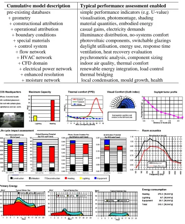
To further support inter-disciplinary working, it is possible to collate the different aspects of performance and present these in the form of an Integrated Performance View (IPV). As shown in Figure 2, an IPV might typically cover issues such as seasonal fuel use, gaseous emissions, thermal/visual comfort, daylight utilisation, renewable energy contribution and so on. Citherlet (2001) has extended the integrated performance modelling approach by adding a life cycle impact assessment procedure.
At present a significant number of modelling systems exist that may be used to address building performance. Details on these systems are available elsewhere (DOE 2002). With the advent of the EU Energy Performance of Buildings Directive (www.diag.org.uk), many of these systems are being adapted to automatically generate compliance information and present the result in a standard format.
Building Simulation Theory
The integrated simulation approach gives rise to an increased computational burden. To accommodate the conflation of the different technical domains while minimising this burden, ESP-r employs the same basic modelling approach throughout coupled to a modular solution approach.
Control Volume Modelling
The building systems are broken down into small control volumes (CV) within which properties such as mass, energy, momentum and contaminant flow are represented mathematically. While the characteristics of CVs can vary – homogeneous or non-homogeneous, solid or fluid, size and shape – the conservation principle can be uniformly applied as appropriate. CVs are used to model a building in whole or part while including the multiplicity of interacting processes.
CV equations represent the fundamental physical processes occurring within the building. Within ESP-r, related sets of equations are grouped and each group
processed by a tailored solver that is optimised for the equation set type. Solution of the equation sets, with real weather data and user defined control objectives as boundary conditions, gives an integrated view of performance over time.
A particular attraction of the CV approach is that the same physical process can be modelled at different levels of detail. For example, the air within a zone may initially be modelled as a single control volume, which corresponds to the assumption of well-mixed air. Later, this single CV can be replaced by multiple CVs to facilitate network air flow or high resolution CFD.
Modular Solution
The set of equations associated with each technical domain are solved by optimised methods that are aligned to the specific nature of the domain equations – sparse, linear, non-linear, mathematically stiff and so on. No attempt is made to concurrently solve the whole system equation set. Instead, the domain equations are solved independently under the control of a supervisory routine that respects the inter-domain couplings. The integrated solution of all domains therefore requires the co-ordinated application of domain solvers.
Building Thermal Processes
The conductive, convective and radiation exchanges associated with a building’s constructions and spaces are established as a set of energy balance equations and a direct solution method applied. The approach is based on a semi-implicit scheme, which is second-order time accurate, unconditionally stable for all space and time steps and allows time dependent problem parameters. An optimised numerical technique is employed to solve the system equations simultaneously, while keeping the required computation to a minimum.
Construction Heat and Moisture Flow
modelled in one-dimension. The resulting CV equations are non-linear and so are solved by an iterative method, with linear under-relaxation employed to prevent convergence instabilities in the case of strong non-linearity or where discontinuities occur in the moisture transfer rate at the maximum relative humidity due to condensation.
Air Flow
For multi-zone problems a nodal network may be invoked to model inter-zone air flow, including infiltration and mechanical ventilation. The approach is based on the solution of the steady-state, one dimensional, Navier-Stokes equation assuming mass conservation and incompressible flow. The result is a set of non-linear equations representing the conservation of mass. To solve these equations, each non-boundary node is assigned an arbitrary pressure and the connecting components' flow rates determined from an empirical mass flow equation. The nodal mass flow rate residuals for the current iteration are then determined and used to establish nodal pressures corrections. The process iterates to convergence.
Intra-Zone Air Movement
The network approach may also be used to model air flow within zones, where the zone air is represented by multiple CVs. However, there are limitations to this approach. First, there is no way to account for the conservation of momentum in the flow and so this modelling method is not applicable for driving flows. Second, the inter-volume couplings are characterised as a function of pressure difference and this requires the specification of a discharge coefficient and little research has been done to determine applicable values. ESP-r therefore employs a built-in CFD model for intra-zone air flow simulation.
Flow inside a room is characterised by a set of time-averaged conservation equations for the three spatial velocities, temperature and contaminant concentration. For turbulent flows two additional equations are added, for turbulence intensity and its rate of dissipation. As with the building thermal domain, these conservation equations are discretised by the finite volume method (Negraõ 1995; Versteeg and Malalasekera 1995) to obtain a set of linear equations. Because these equations are
strongly coupled and highly non-linear, they are solved iteratively for a given set of boundary conditions using the SIMPLEC method (Patankar 1980; Van Doormal and Raithby 1984) in which the pressure of each cell is linked to the velocities connecting with surrounding cells in a manner that conserves continuity. The method accounts for the absence of an equation for pressure by establishing a modified form of the continuity equation to represent the pressure correction that would be required to ensure that the velocity components determined from the momentum equations move the solution toward continuity. This is done by using a guessed pressure field to solve the momentum equations for intermediate velocity components and then using these velocities to estimate the required pressure field correction from the modified continuity equation. The energy equation, and any other scalar equations (e.g. for species concentration), are then solved and the process iterates until convergence is attained. To avoid numerical divergence, under-relaxation is applied to the pressure correction terms.
HVAC Systems
The CV technique is also be used to derive equation sets describing a building’s plant network. This network consists of a coupled group of plant component models, each described by one or more CV. Mclean (1982), Tang (1985), Hensen (1991), Aasem (1993) and Chow et al (1998) have applied the CV modelling technique to a variety of plant components. The resulting library of models allows the simulation of air conditioning systems, hot water heating systems and mixed air/hot water systems as a network in ESP-r.
The equations derived for plant are of a form that allows their solution using an efficient, direct method. The solution of the plant matrix is dictated by control interaction, where the state of the system components is adjusted to bring about a desired control objective. The sensed node for plant control may be another plant component or state in the building model, e.g. cooling coil operation may be controlled based on zone relative humidity.
Electrical Power Flow
resolve electrical power flows (Kelly 1998). The electrical circuit is conceived as a network of CVs (nodes) representing the junctions between conducting elements and locations where power is extracted to feed loads, or added from the supply network or embedded renewable energy components. Application of Kirchhoff's current law to network nodes results in equations representing the real and reactive power balance at each node. The solution procedure is identical to that employed for inter-zone air flow except that the state variable is voltage, not pressure, and two equation-sets must be solved for real and reactive power flow.
Variable Frequency Processing
The various equation sets comprising the overall model represent systems with very different time constants: in the fabric of the building, temperatures change slowly over a period of hours, while in the plant system, temperatures and flow change more rapidly and certainly within minutes. A feature of the modular solution process is the ability to independently vary the solution frequency of each equation set, enabling the solution to capture the dynamics of a particular system.
Solution Co-ordination
To orchestrate the solution process, domain-aware conflation controllers are imposed on the different iterations. Consider, for example, the linking of the building thermal, network air flow and CFD models (Beausoleil-Morrison 2000). At the start of a time-step, the zero-equation turbulence model of Chen and Xu (1998) is used in investigative mode to determine the likely surface flow regimes (buoyant, fully/weakly turbulent etc). The result is used to select appropriate surface boundary conditions and the estimated eddy viscosity distribution is used to initialise turbulence intensity and its rate of dissipation.
On the basis of the investigative simulation, the nature of the flow at each surface is evaluated from the local Grashof and Reynolds Numbers, which indicate how buoyant and how forced the flow is respectively. Where buoyancy forces are insignificant, the buoyancy term in the z-momentum equation is discarded to improve solution convergence. Where free convection predominates, the log-law wall functions are replaced by wall
functions developed by Yuan et al (1993) and constant boundary conditions imposed where the surface is vertical; otherwise a convection coefficient correlation is prescribed (this means that the thermal domain will influence the flow domain but not the reverse). Where convection is mixed, the log-law wall functions are replaced by a convection coefficient boundary condition. Where forced convection predominates, the ratio of the eddy viscosity to the molecular viscosity, as determined from the investigative simulation, is used to determine how turbulent the flow is locally.
The iterative solution of the flow equations is re-initiated for the current time-step. For surfaces where convection coefficient correlations are active, these are shared with the building thermal model to impose the surface heat flux on the CFD solution. Where such correlations are not active, the CFD-derived convection coefficients are inserted into the building thermal model's surface energy balance.
Where an air flow network is active, the node representing the room is removed and new connection(s) added to effect a coupling with the appropriate domain cell(s) (Negraõ 1995; Clarke et al 1995).
Development Trends
The ESP-r approach has proved to be resilient when applied to a range of problems; the real issue is whether the approach will accommodate future user requirements.
The modelling of new phenomena often only requires minor changes to the existing set-up. For example, modelling of new thermal processes occurring in the building fabric requires only the implementation of a new source term, the adjustment of existing equation coefficients or incorporating both together through a control function. This approach was adopted to implement phase change materials and the modelling of double skin facades. It was also used to model innovative components such as light sensitive shading devices and hybrid PV.
moisture flow modelling from 1D to 3D to facilitate more accurate representations. This would be an important addition to ESP-r because it would allow the growth of mould to be predicted. However, it would not be appropriate to couple a detailed fabric model to a lumped air volume as the detail of the former model would be lost. Instead, the detailed fabric model must be directly coupled to a CFD domain. This requires extensions to the linkages between the building fabric (thermal and moisture) and CFD domains. Such an extension is at the planning stage.
While ESP-r’s integrated CFD model can be readily applied to many air quality issues with minor adaptation, other developments will require additional equations and so will impact upon the solution procedure. For example, the CFD model is presently incapable of handling small solid particulates that have appreciable mass. Two particle dispersion/deposition modelling methods are being considered for implementation: treating the particles as a continuum or particle tracing using Lagrange coordinates. A prototype of the former techniquemodel has recently been implemented to enable the modelling of small particles in flows with Stoke’s number significantly less than 1 (Kelly and Macdonald 2004).
The modelling of fire/smoke requires that extra equations be added to handle combustion reactions and the transport of combustion products (e.g. via the implementation of mixture fraction or grey gas radiation transport models). Such adjustments can be readily implemented within the existing code since the governing equations are of diffusive type and so can be treated in the same way as the energy and species diffusion equations.
In relation to the network air flow model, possible improvements include the introduction of a pressure capacity term to the mass balance equations to facilitate the modelling of compressible flows, and the introduction of transport delay terms to network connections.
Further developments are possible to the electrical model, especially in relation to the modelling of micro-generation systems operating within a mico-grid, where control
actions are based on electrical criteria such as voltage regulation, network stability and phase balancing. Control of this type will require the creation of a high-level supervisor to iteratively couple the electrical and non-electrical domains in order to balance the conflicting demands of local comfort and community benefit. In relation to micro-grids, some challenges remain to be resolved, including the development of demand management algorithms that switch certain loads within the context of renewable power trading. The simultaneous modelling of multiple buildings and micro-generation systems will also be required. Modelling at this scale is well suited to parallel processing, where different aspects of the model (dwellings, micro-power units and the electrical grid) are allocated to different streams.
The ESP-r approach has proven amenable to the modelling of passive and active renewable energy systems, with the implementation of models of solar thermal collectors (McLean 1982), solar roof ponds (Clarke and Strachan 1994), PV components (Clarke et al 1996) and building-integrated wind turbines (Grant and Kelly 2004). These models are implemented either by utilising ESP-r’s existing building fabric model (e.g. PV) or by developing a component for use within the HVAC network model (e.g. solar thermal collector). Indeed, some of ESP-r’s low-carbon energy models span up to three domains. For example, a PV model typically comprises fabric, flow and electrical constituents.
In the long term, additional solver developments may be implemented to bring about computational efficiencies and thereby assist with the translation of simulation to the early design stage. For example: additional, context-aware solution accelerators may be embedded within the solvers to control their appropriate invocation; parallelism may be introduced to allow the different domains to be established and solved in tandem to reduce simulation times; and network computing might be exploited to allow different aspects of the same problem to be pursued at different locations as an aid to team working.
Finally, it is worth mentioning that no matter how well the technical domains of the building are modelled, the effects of occupancy can vastly alter the physical behaviour and ultimately the predicted energy performance. These effects arise from two avenues: behaviour (e.g. the occupants' response to window opening) and attitude (e.g. the rejection of facilities on other than performance grounds). Developments are underway to address the distributed impacts of occupant actions (e.g. the impact on the network flow, CFD, thermal and lighting domains of window opening).
Conclusions
This paper has summarised the modular approach to multi-domain solution as employed within the ESP-r system. Several possible technical developments were then outlined as required by new user demands that imply a need to extend and deepen future building performance analysis. The modular approach was shown to be well suited to such future adaptations.
References
Aasem E O (1993), ‘Practical simulation of buildings and air-conditioning systems in the transient domain’, PhD Thesis, Glasgow: University of Strathclyde.
Beausoleil-Morrison I (2000), ‘The Adaptive Coupling of Heat and Air Flow Modelling within Dynamic Whole-Building Simulation’, PhD Thesis, Glasgow: University of Strathclyde.
Beausoleil-Morrison I, Cuthbert D, Deuchars G, McAlary G (2002), ‘The Simulation of Fuel Cell Cogeneration Systems in Residential Buildings’, Proc. eSim, bi-annual conf., IBPSA-Canada.
Chen Q and Xu W (1998), ‘A Zero-Equation Turbulence Model for Indoor Airflow Simulation’, Energy and Buildings, 28(2), pp137-44.
Chow T T, Clarke J A and Dunn A (1998), ‘Theoretical Basis of Primitive Part Modelling’, ASHRAE Trans., 104(2).
CIBSE (1998) Applications Manual AM11: Building energy and environmental modelling (London: Chartered Institute of Buildings Services Engineers) ISBN 0 900953 85 3
Citherlet S (2001), ‘Towards the holistic assessment of building performance based on an integrated simulation approach’, PhD Thesis (Lausanne: Swiss Federal Institute of Technology)
Clarke J A (2001), Energy Simulation in Building
Design (2nd Edn), London:
Butterworth-Heinneman.
Clarke J A, Hand J W, Johnstone C, Kelly N, Strachan P A (1996), ‘The Characterisation of Photovoltaic-Integrated Building Facades Under Realistic Operating Conditions’, Proc. 4th European Conference on Solar Energy in Architecture and Urban Planning, Berlin, 26-29 March.
Clarke J A, Dempster W M and Negraõ C (1995), ‘The Implementation of a Computational Fluid Dynamics Algorithm within the ESP-r System’, Proc. Building Simulation '95, Madison WI, pp166-75.
Clarke J A and Strachan P A (1994), ‘Simulation of Conventional and Renewable Building Energy Systems’, Proc. 3rd World Renewable Energy Congress, Part II, pp1178-1189, Reading.
DOE 2002 (www.eren.doe.gov/buildings/tools_ directory/).
Ferguson A, Kelly N J (2006), ‘Modelling Building-Integrated Stirling CHP Systems’, Proc. eSim, bi-annual conf., IBPSA-Canada.
Grant A D and Kelly N J (2004), ‘A Ducted Wind Turbine Model for Building Simulation’,
Building Services Engineering Research and Technology, V25(4), pp339-350.
Hand J W (1998) ‘Removing barriers to the use of simulation in the building design professions’, PhD Thesis, University of Strathclyde.
Hensen J L M (1991), ‘On the thermal interaction of building structure and heating and ventilating system’, PhD Thesis, Eindhoven: University of Technology.
with Building Simulation’, PhD Thesis, Glasgow: University of Strathclyde.
Kelly N J and Macdonald I (2004), ‘Coupling CFD and Visualisation to Model The Behaviour and Effect on Visibility of Small Particles In Air’, Proc. eSim bi-annual conf., pp153-160, Vancouver, 9-11 June.
McLean D J (1982), ‘The simulation of solar energy systems’, PhD Thesis, Glasgow: University of Strathclyde.
Nakhi A E (1995), ‘Adaptive Construction Modelling Within Whole Building Dynamic Simulation’, PhD Thesis, Glasgow: University of Strathclyde.
Negraõ C O R (1995), ‘Conflation of Computational Fluid Dynamics and Building
Thermal Simulation’, PhD Thesis, Glasgow: University of Strathclyde.
Tang D (1985), ‘Modelling of Heating and Air Conditioning System’ ,PhD Thesis, University of Strathclyde, Glasgow.
Van Doormal J P and Raithby G D (1984), ‘Enhancements of the SIMPLE Method for Predicting Incompressible Fluid Flows’, Numerical Heat Transfer, 7, pp147-63.
Versteeg H K and Malalasekera W (1995), An introduction to Computational Fluid Dynamics: The Finite Volume Method, England: Longman.
[image:8.595.112.488.300.755.2]Yuan X, Moser A and Suter P (1993), ‘Wall Functions for Numerical Simulation of Turbulent Natural Convection Along Vertical Plates’, Int. J. Heat Mass Transfer, 36(18), pp4477-85.
Table 1: Mapping problem description to performance results.
Figure 2: Multi-variate performance summaries support team working.
Cumulative model description Typical performance assessment enabled
pre-existing databases + geometry
+ constructional attribution + operational attribution + boundary conditions + special materials + control system + flow network + HVAC network + CFD domain
+ electrical power network + enhanced resolution + moisture network
simple performance indicators (e.g. U-value) visualisation, photomontage, shading material quantities, embodied energy casual gains, electricity demands
illuminance distribution, no-systems comfort photovoltaic components, switchable glazings daylight utilisation, energy use, response time ventilation, heat recovery evaluation
psychrometric analysis, component sizing indoor air quality, thermal comfort renewable energy integration, load control thermal bridging
.
Figure 1: Progressive aspects of the integrated building modelling approach.
a b c d e
1
2
3