White Rose Research Online URL for this paper:
http://eprints.whiterose.ac.uk/146181/
Version: Published Version
Article:
Davis, Robert Ian orcid.org/0000-0002-5772-0928 and Cucu-Grosjean, Liliana (2019) A
Survey of Probabilistic Schedulability Analysis Techniques for Real-Time Systems. LITES:
Leibniz Transactions on Embedded Systems. pp. 1-53. ISSN 2199-2002
eprints@whiterose.ac.uk https://eprints.whiterose.ac.uk/ Reuse
This article is distributed under the terms of the Creative Commons Attribution (CC BY) licence. This licence allows you to distribute, remix, tweak, and build upon the work, even commercially, as long as you credit the authors for the original work. More information and the full terms of the licence here:
https://creativecommons.org/licenses/
Takedown
If you consider content in White Rose Research Online to be in breach of UK law, please notify us by
for Real-Time Systems
Robert I. Davis
University of York, UK and Inria, France rob.davis@york.ac.uk
Liliana Cucu-Grosjean
Inria, France liliana.cucu@inria.fr
Abstract
This survey covers probabilistic timing analysis techniques for real-time systems. It reviews and critiques the key results in the field from its ori-gins in 2000 to the latest research published up to the end of August 2018. The survey provides a taxonomy of the different methods used, and a classification of existing research. A detailed review is provided covering the main subject areas: static
probabilistic timing analysis, measurement-based probabilistic timing analysis, and hybrid methods. In addition, research on supporting mechanisms and techniques, case studies, and evaluations is also reviewed. The survey concludes by identifying open issues, key challenges and possible directions for future research.
2012 ACM Subject Classification Software and its engineering→Software organization and properties,
Software and its engineering→Software functional properties, Software and its engineering→Real-time
schedulability, Computer systems organization→Real-time systems
Keywords and Phrases Probabilistic, real-time, timing analysis
Digital Object Identifier 10.4230/LITES-v006-i001-a003
Received 2018-01-04Accepted 2019-02-26Published 2019-05-14
1
Introduction
Systems are characterised as real-time if, as well as meeting functional requirements, they are required to meet timing requirements. Real-time systems may be further classified ashard real-time, where failure to meet their timing requirements constitutes a failure of the system; orsoft
real-time, where such failure leads only to a degraded quality of service. Today, both hard and soft real-time systems are found in many diverse application areas including; automotive, aerospace, medical systems, robotics, and consumer electronics.
Real-time systems are typically implemented via a set of programs, also referred to as tasks, which are executed on a recurring basis. The programs used in a real-time system have afunctional
In keeping with the majority of the work on program timing behaviour, in the following we consider programs that are run without interruption or preemption and without any interference from other programs that could be running on the same or different processor cores (i.e. no multi-threading and no cross-core interference). We return to this point in the conclusions.
The timing behaviour of a program with deterministic functionality depends on both the input state, and the initial values of hardware state variables, referred to as thehardware state. Examples of hardware state variables include the contents of internal buffers, pipelines, caches, scratchpads, and certain register values. While the hardware state may affect the timing behaviour of the program, it has no effect on the functional behaviour. A hardware platform is referred to as time-predictable if it always takes the same amount of time to execute a deterministic program when starting from the same input state and the same hardware state. By contrast, a
time-randomised hardware platform may take a variable amount of time to execute such a program when starting from the same input state and hardware state, due to the behaviour of underlying random elements in the hardware1.
1.1
Conventional Timing Analysis Techniques
Understanding the timing behaviour of each program is fundamental to verifying the timing requirements of a real-time system. Key to this istiming analysis, which seeks to characterise the amount of time that each program can take to execute on the given hardware platform. Typically, this is done by upper bounding or estimating theWorst-Case Execution Time.
◮Definition 1. TheWorst-Case Execution Time (WCET)of a program is an upper bound on
the execution time of that program for any valid input state and initial hardware state (i.e. the WCET is an upper bound on the execution time for any single run of the program, and there is at least one run of the program that can realise the WCET).
The methods traditionally used for timing analysis can be classified into three main categories:
Static Analysis: These methods do not execute the program on the actual hardware or on a simulator. Rather they analyse the code for the program and some annotations (providing information about input values), along with an abstract model of the hardware. Typically static analysis proceeds in three steps. First, control flow analysis is used to derive constraints on feasible paths, including loop bounds. Second, micro-architectural analysis is used to provide an over-approximation of the program execution on the feasible paths, accounting for the behaviour of hardware features such as pipelines and caches. Third, path analysis uses integer linear programming (ILP) to combine the results of control flow analysis and micro-architectural analysis, and so derive an upper bound on the WCET of the program. To derive an upper bound on the WCET static analysis has to determine properties relating to the dynamic behaviour of the program without actually executing it. In practice, it may not be possible to precisely determine all of these properties due to issues of tractability and decidability. For example determining the precise cache contents at a given program point may not be possible when there is a dependency on the input values. Properties which cannot be precisely determined must be conservatively approximated to ensure that the computed WCET remains a valid upper bound; however, such approximations may lead to significant pessimism. For advanced hardware platforms, there are two main challenges for static analysis methods. Firstly, obtaining and validating all of the information necessary to build an accurate
1
model of the hardware components that impact program execution times. Secondly, modelling those components and their interactions without substantial loss of precision in the derived WCET upper bound.
Dynamic or Measurement-Based Analysis: These methods derive an estimate of the WCET by running the program on the actual hardware or on a cycle-accurate timing simulator. A measurement protocol provides test vectors (sets of input values) and initial hardware configurations that are used to exercise a subset of the possible paths through the code, as well as the possible hardware states that may affect the timing behaviour2. The execution times for multiple runs of the program are collected and the maximum observed execution time recorded. This value may be used as a (lower bound) estimate of the WCET, or alternatively, an engineering margin (e.g. 20%) may be added to give an estimate of the WCET. This margin comes from industrial practice and engineering judgement [129]; however, there is no guarantee that it results in an upper bound on the actual WCET. For complex programs and advanced hardware platforms, the two main challenges for measurement-based analysis methods both involve designing an appropriate measurement protocol. Firstly, if it were known which values for the input variables and software state variables would lead to the WCET, then the measurement protocol could ensure that those values were present in the test vectors used; however, typically these values are not known and cannot easily be derived. Secondly, it may not be known, or easy to derive, which initial hardware states will lead to the WCET; it may also be difficult to force the hardware into a particular initial state. Nevertheless, measurement-based analysis is commonly used in industry and may give engineers a useful perspective on the timing behaviour of a program.
Hybrid Analysis: These methods combine elements of both static analysis and measurement-based analysis. For example, a hybrid approach may record the maximum observed execution time for short sub-paths through the code, and then combine these values using information obtained via static analysis of the program’s structure (e.g. the control flow graph) to estimate the WCET. The aim of hybrid analysis is to overcome the disadvantages of both static and dynamic methods. By measuring execution times for short sub-paths through the code, hybrid methods avoid the need for a model of the hardware, which may be difficult to obtain and to validate. By using static analysis techniques to determine the control flow graph, the problem of having to find input values that exercise the worst-case path is ameliorated. Instead, the measurement protocol can focus on ensuring that measurements are obtained for all sub-paths, i.e. structural coverage, which is far simpler to achieve than full path coverage. Nevertheless, hybrid methods still inherit many of the challenges of measurement-based methods. On advanced hardware (e.g. with pipelines and caches) the execution time of a sub-path may be dependent on the execution history, and hence on the previous sub-paths that were executed. This exacerbates the problem of composing the overall WCET estimate from observations for individual sub-paths, and may degrade the precision of that estimate. In general, today’s hybrid methods cannot guarantee to upper bound the WCET; however, the estimates they produce may be more accurate than those based on measurements alone.
During the past two decades, the hardware platforms used, or proposed for use, in real-time systems have become increasingly more complex. Architectures include advanced hardware acceleration features such as pipelines, branch prediction, out-of-order execution, caches, write-buffers, scratchpads, and multiple levels of memory hierarchy. These advances, along with increasing software complexity, greatly exacerbate the timing analysis problem. Most acceleration
2
features are designed to optimise average-case rather than worst-case behaviour and can result in significant variability in execution times. This is making it increasingly difficult, if not impossible, to obtain tight WCET estimates3 from conventional static timing analysis methods that seek to provide an upper bound on the WCET. Further, increases in software and hardware complexity make it difficult to design measurement protocols capable of ensuring that the worst-case path(s) through the code are exercised, and that the worst-case hardware states are encountered when using measurement-based and hybrid analyses. (Appendix A provides further discussion of measurement protocols).
1.2
Probabilistic Timing Analysis Techniques
Probabilistic timing analysis4differs from traditional approaches in that it lifts the characterisation
of the timing behaviour of a program from the consideration of a single run, to the consideration of a repeating sequence of many runs, referred to as ascenario, and hence lifts the results from a scalar value (the WCET) to a probability distribution (the pWCET distribution, defined in Section 2.1). Traditional timing analysis methods aim to tightly upper bound the execution time that could occur for a single run of a program out of all possible runs. Similarly, probabilistic timing analysis methods aim to tightly upper bound the distribution of execution times that could potentially occur for some scenario of operation, out of all possible scenarios of operation.
Research into probabilistic timing analysis can be classified into five main categories. This classification forms the basis for the main sections of this survey. Note, for ease of reference we have numbered these categories below, starting at 3, to match the section of survey.
3. Static Probabilistic Timing Analysis (SPTA): Similar to traditional static analyses, SPTA methods do not execute the program on the actual hardware or on a simulator. Instead they analyse the code for the program and information about input values, along with an abstract model of the hardware behaviour. The difference is that SPTA methods account for some form of random behaviour in either the hardware, the software, or the environment (i.e. the inputs) by using probability distributions, and therefore construct an upper bound on the pWCET distribution rather than a upper bound on the WCET. In common with traditional static analyses, SPTA methods have to determine properties relating to the dynamic behaviour of the program without actually executing it. Here, the conservative approximation of properties which cannot be precisely determined (e.g. cache states in a random replacement cache) may lead to significant pessimism in the estimated pWCET distribution. The two main challenges for SPTA methods are obtaining and validating the information necessary to build an accurate model of the hardware components; and modelling those components and their interactions without substantial loss of precision in the upper bound pWCET distribution derived.
4. Measurement-Based Probabilistic Timing Analysis (MBPTA): Today, most of the current MBPTA methods use Extreme Value Theory (EVT) to make a statistical estimate of the pWCET distribution of a program. This estimate is based on a sample of execution time observations obtained by executing the program on the hardware or a cycle accurate simulator according to ameasurement protocol. The measurement protocol samples some scenario(s) of operation, i.e. it executes the program multiple times according to a set of feasible input states and initial hardware states. As with traditional measurement-based analysis methods, the
3
By a tight WCET estimate we mean one that is relatively close to the actual WCET, for example perhaps no more than 10-20% larger.
4
main challenge for MBPTA methods involves designing an appropriate measurement protocol. In particular, in order for the estimated pWCET distribution derived by EVT to be valid for a future scenario of operation, then the sample of input states and hardware states used for analysis must berepresentativeof those that will occur during that future scenario of operation. An important issue here is that there may not be a single sample of input states and hardware states that is representative of all possible future scenarios of operation.
5. Hybrid Probabilistic Timing Analysis (HyPTA): These methods combine in some way both statistical and analytical approaches. For example by taking measurements at the level of basic blocks or sub-paths, and then composing the results (i.e. the estimated pWCET distributions for the sub-paths) using structural information obtained from static analysis of the code.
6. Enabling mechanisms: These mechanisms aim to facilitate the use of one or other of the above analysis methods.
7. Evaluation: Case studies, benchmarks, and metrics, which aim to evaluate the efficiency, effectiveness, and applicability of probabilistic timing analysis methods.
0 5 10 15 20 25 30
N
u
m
b
e
r
o
f
p
u
b
li
ca
ti
o
n
s
Publication Date
7 Case Studies, Benchmarks and Evaluation
6 Enabling Mechanisms and Techniques
5 Hybrid Techniques for Probabilistic Timing Analysis (HyPTA)
4 Measurement-Based Probabilistic Timing Analysis (MBPTA)
[image:6.595.81.500.304.617.2]3 Static Probabilistic Timing Analysis (SPTA)
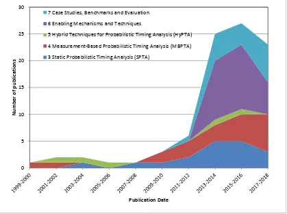
Figure 1Intensity of research in the different categories corresponding to Sections 3 to 7 of this survey. The research in these categories is summarised by authors and citations in Table 1. Note the sub-categories correspond to the subsections of this survey.
Table 1Summary of publications from different authors in the categories described in the main sections and subsections of this survey.
3 Static Probabilistic Timing Analysis (SPTA) 3.1 SPTA based on Probabilities from Inputs David and Puaut [35], Liang and Mitra [86] 3.2 SPTA based on Probabilities from Faults
Hofig [62], Hardy and Puaut [58, 59], Chen et al. [31, 29]
3.3 SPTA based on Probabilities from Random Replacement Caches
Quinones et al. [106], Burns and Griffin [23], Cazorla et al. [26], Davis et al. [39], Altmeyer and Davis [7], Altmeyer et al. [6], Griffin et al. [52], Lesage et al. [83, 82], Chen and Beltrame [28], Chen et al. [30]
4 Measurement-Based Probabilistic Timing Analysis (MBPTA) 4.1 EVT and i.i.d. observations
Burns and Edgar [22], Edgar and Burns [45], Hansen et al. [57], Griffin and Burns [51], Lu et al. [89, 90], Cucu-Grosjean et al. [34]
4.2 EVT and observations with dependences
Melani et al. [93], Santinelli et al. [112], Berezovskyi et al. [16, 15], Guet et al. [53, 54], Fedotova et al. [47], Lima and Bate [87]
4.3 EVT and representativity
Lima et al. [88], Maxim et al. [92], Santinelli et al. [110], Santinelli and Guo [111], Guet et al. [55], Abella et al. [3], Milutinovic et al. [101]
5 Hybrid Techniques for Probabilistic Timing Analysis (HyPTA) 5.1 HyPTA and the Path Coverage Problem
Bernat et al. [19, 18, 17], Kosmidis et al. [70], Ziccardi et al. [136]
6 Enabling Mechanisms and Techniques 6.1 Caches and Hardware Random Placement
Kosmidis et al. [68, 69, 67], Slijepcevic et al. [120], Anwar et al. [9], Hernandez et al. [61], Trillia et al. [127], Benedicte et al. [11]
6.2 Caches and Software Random Placement Kosmidis et al. [72, 73, 71, 78]
6.3 Cache Risk Patterns with Random Placement
Abella et al. [4], Benedicte et al. [13, 14], Milutinovic et al. [98, 99, 97, 100] 6.4 Buffers, Buses and other Resources
Slijepcevic et al. [119], Cazorla et al. [27], Kosmidis et al. [74], Jalle et al. [65], Panic et al. [102], Agirre et al. [5], Hernandez et al. [60], Slijepcevic et al. [117, 118], Benedicte et al. [12]
7 Case Studies, Benchmarks and Evaluation 7.1 Critiques
Reineke [108], Mezzetti et al. [96], Stephenson et al. [123], Gil et al. [49] 7.2 Case Studies and Evaluation
and then increased rapidly in the decade from 2010. Inline with this the number of publications on the main theme of measurement-based probabilistic timing analysis (Section 4) has steadily increased since 2009/2010. Work on static probabilistic timing analysis (Section 3) peaked during the period 2013–2016, coinciding with research effort on the EU Proxima project5. Also, as a
result of that project, there was a significant peak in research on enabling techniques aimed at facilitating the use of MBPTA (Section 6). More recently, in 2017/2018, the focus has been on extending MBPTA to more complex systems and exploring the effectiveness of the approach via case studies and benchmarks (Section 7).
Before moving to the sections of this survey which review the literature, we first discuss (in Section 2) fundamental concepts and methods relating to probabilistic timing analysis.
Note that conventional timing analysis techniques aimed at providing an upper bound on the WCET value as the solution to the timing analysis problem are outside of the scope of this survey, they are reviewed in detail by Wilhelm et al. [133].
2
Fundamental Concepts and Methods
The termprobabilistic real-time systemsis used to refer to real-time systems where one or more of the parameters, such as program execution times, are modelled by random variables. Although a parameter is described (i.e.modelled) by a random variable, this does not necessarily mean that the actual parameter itself exhibits random behaviour or that there is necessarily any underlying random element to the system that determines its behaviour. The actual behaviour of the parameter may depend on complex and unknown or uncertain behaviours of the overall system. As an example, the outcome of a coin toss can be modelled as a random variable with heads and tails each having a probability of 0.5 of occurring, assuming that the coin is fair. However, the actually process of tossing a coin does not actually have a random element to it. The outcome could in theory be predicted to a high degree of accuracy if there were sufficiently precise information available about the initial state and the complex behaviour and evolution of the overall physical processes involved. There are however many useful results that can be obtained by modelling the outcome of a coin toss as a random variable. The same is true of the analysis of probabilistic real-time systems.
In this section, we first discuss a fundamental and often misunderstood concept in probabilistic timing analysis,probabilistic Worst-Case Execution Time (pWCET)distributions. The remainder of the section then provides an outline of the two main approaches to obtaining pWCET distribu-tions,Static Probabilistic Timing Analysis (SPTA)andMeasurement-Based Probabilistic Timing Analysis (MBPTA).
2.1
probabilistic Worst-Case Execution Time (pWCET)
The termprobabilistic Worst-Case Execution Time (pWCET)distribution has been used widely in the literature, with a number of different definitions given. Below, we provide an overarching definition of the term. (We use calligraphic characters, such asX, to denote random variables).
◮Definition 2. Theprobabilistic Worst-Case Execution Time (pWCET)distribution for a program
is the least upper bound, in the sense of the greater than or equal to operator(defined below), on the execution time distribution of the program for every valid scenario of operation, where ascenarioof operation is defined as an infinitely repeating sequence of input states and initial hardware states that characterise a feasible way in which recurrent execution of the program may occur.
5
◮Definition 3. (From Diaz et al. [44]) The probability distribution of a random variable X is greater than or equal to(i.e. upper bounds) that of another random variableY (denoted byX Y) if the Cumulative Distribution Function (CDF) ofX is never above that ofY, or alternatively, the 1-CDF ofX is never below that ofY.
Graphically, Definition 2 means that the 1 - CDF of the pWCET distribution is never below that of the execution time distribution for any scenario of operation. Hence the 1 - CDF or
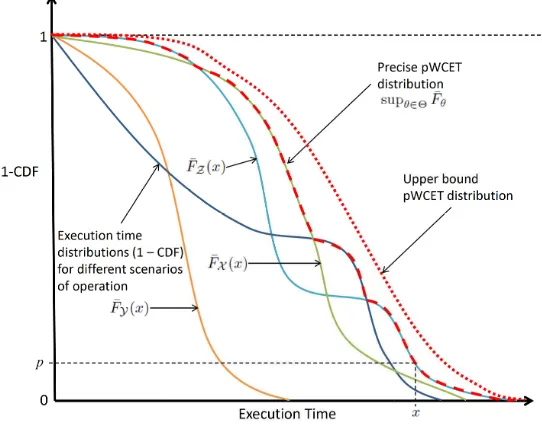
[image:9.595.165.436.254.471.2]exceedance funtion of the pWCET distribution may be used to determine an upper bound on the probabilitypthat the execution time of a randomly selected run of the program will exceed an execution time budgetx, for any chosen value of x. This upper bound is valid for any feasible scenario of operation.
Figure 2Exceedance function or 1-CDF for the pWCET distribution of a program, and also execution time distributions for specific scenarios of operation.
Figure 2 illustrates the execution time distributions of a number of different scenarios of operation (solid lines), the precise pWCET distribution (red dashed line) which is the least upper bound (i.e. the point-wise maxima of the 1 - CDF) for all of these distributions, and also some arbitrary upper bound pWCET distribution (red dotted line) which is a pessimistic estimate of the precise pWCET. Also shown (on the y-axis) is an upper boundpon the probability that any randomly selected run of the program will have an execution time that exceedsx(on the x-axis). The value xis referred to as the pWCET estimate at a probability of exceedance ofp. (More formally, the least upper bound pWCET distribution is given by supθ∈ΘF¯θ, where ¯Fθ is the 1
-CDF for scenario of operationθ, and Θ is the space of all valid scenarios of operation).
Note that the greater than or equal to relation between two random variables does not provide a total order, i.e. for two random variablesX andZit is possible thatX Z andZX. Hence the precise pWCET distribution may not correspond to the execution time distribution for any specific scenario. This can be seen in Figure 2, considering the execution time distributions
The WCET upper bounds all possible execution times for a program, independent of any particular run of the program. Similarly, the pWCET distribution upper bounds all possible execution time distributions for a program, independent of any particular scenario of operation. We note that the term pWCET is open to misinterpretation and is often misunderstood. To clarify, it doesnot refer to the probability distribution of the worst-case execution time, since the WCET is a single value. Rather informally, following Definition 2, the pWCET may be thought of as the “worst-case” (in the sense of upper bound) probability distribution of the execution time for any scenario of operation.
Below, we provide some simple hypothetical examples that illustrate the meaning of the pWCET distribution.
Consider a program A running on time-randomised hardware. Further, assume that the program has two paths which may be selected based on the value of an input variable. The discrete probability distributionsX and Y of the execution time of each path may be described byprobability mass functionsas follows:
X =
10 20 30 40 0.4 0.3 0.2 0.1
Y =
20 30 40 50 0.8 0.15 0.04 0.01
Indicating, among other things, that there is a probability of 0.1 that the execution time of the first path is 40 and a probability of 0.01 that the execution time of the second path is 50.
TheComplementary Cumulative Distribution Function(1-CDF) orExceedance Functiondefined as ¯FX(x) =P(X > x) is given by:
¯
FX =
0 10 20 30 40 1 0.6 0.3 0.1 0
¯
FY =
0 10 20 30 40 50 1 1 0.2 0.05 0.01 0
The precise pWCET distribution for the two paths can be found by taking the point-wise maxima of their exceedance functions. Hence:
pW CET =
0 10 20 30 40 50 1 1 0.3 0.1 0.01 0
Note that the above pWCET distribution is precise on the assumption that repeatedly executing one path or the other or any combination of them is a valid scenario of operation, otherwise it may be that it is an upper bound rather than the precise pWCET.
Observe that the program has a WCET of 50, which equates to the last value in the pWCET distribution (where the 1-CDF becomes zero). The pWCET distribution gives more nuanced information than this single value, as it upper bounds the probability of occurrence of the extreme execution time values (e.g. 30, 40, and 50) that occur rarely and form the tail of the distribution.
Execution on time-randomised hardware is not the only way in which a non-degenerate6
pWCET distribution can arise. As an alternative, consider another programB that implements a software state machine with four states and hence four paths that runs on time-predictable hardware. Here the main factor which affects the execution time is the path taken, which is determined by the value of the software state variable. For this program, all valid scenarios of operation involve the software state variable cycling through its four possible values in order, and hence the four possible paths executing in order on any four consecutive runs of the program. Further, assume that there is a small variability in the execution time of each path depending on the value of some input variable, which may take any value on any run. Hence the execution
6
times of the different paths are 10±2, 20±2, 30±2, and 40±2, each with a probability of 0.25. For this program, the pWCET distribution valid for any scenario of operation is:
pW CET =
0 12 22 32 42 1 0.75 0.5 0.25 0
Finally, consider a programCwhich again runs on time-predictable hardware. This program has an input variablev which may take one of four values selecting one of four different paths. The execution times of the paths are 10, 20, 30, and 40. Further, we are given some additional information about all the valid scenarios of operation, over a large number of runs of the program, the first 3 input values occur with the same probability, while the 4th is a fault condition that occurs at most 1% of the time. The pWCET distribution is as follows:
pW CET =
0 10 20 30 40 1 0.67 0.34 0.01 0
We note that in all three examples, the pWCET distribution upper bounds the execution time distribution for a randomly selected run of the program in any scenario of operation. However, it is not always the case that the pWCET distribution is probabilistically independent of the value realised for the execution time of previous runs of the program. For example in the case of programB, the pWCET distribution does not provide a valid upper bound on the execution time distribution of the programconditional on specific execution times having occurred for previous runs. (If the previous execution time of the program was 30, then the execution time of the current run has a probability of 1 of exceeding 32, since the state variable will increment by 1 and the longest path will be selected with an execution time of 40±2 ). Further, in the case of programC, although the fault condition may occur only 1% of the time, there may well be a cluster of faults. Hence for programsB andC, it is not valid to compose the pWCET distributions using basic convolution to obtain a bound on the interference (total execution time) of two or more runs of the program. This has implications for how the pWCET distribution may be used in probabilistic schedulability analysis, which are discussed in the companion survey on that topic [38].
◮Definition 4. Two random variablesX andY areprobabilistically independent if they describe
two events such that knowledge of whether one event did or did not occur does not change the probability that the other event occurs. Stated otherwise, the joint probability is equal to the product of their probabilitiesP({X =x} ∩ {Y =y}) =P(X =x)·P(Y =y). (In this context, the events are the execution times of runs of the program taking certain values).
We note that while the above simple examples are useful to illustrate the concept of a pWCET distribution, in practice the exceedance probabilities of interest are very small, typically in the range 10−4 to 10−15. These probabilities derive from the acceptable failure rate per hour of
operation for the application considered. (Note, the relationship between failure rates per hour of operation and probabilities of timing failure depend on various factors considered in fault tree analysis, including any mitigations and recovery mechanisms that may be applied in the event of a timing failure [50], see the companion survey [38] for further discussion).
(i) An upper boundpon the probability (with a long-run frequency interpretation) equating to the number of runs expected to exceed the execution time budget xdivided by the total number of runs in a long (tending to infinite) time interval.
(ii) An upper bound pon the probability that the execution time budgetxwill be exceeded on a randomly selected run. (This is broadly equivalent to the above long-run frequency interpretation).
Contrast this with the binary information provided by the WCET. Ifxis greater than or equal to the WCET, then we can expect the budget to never be exceeded. However, ifxis less than the WCET, then we expect the budget to be exceeded on some runs, but we have no information on how frequently this may occur. Hard real-time systems in many application domains can in practice tolerate a small number of consecutive failures of a program to meet its execution time budget, but cannot tolerate long black-out periods when every run fails to complete within its budget. The problem of reconciling requirements on the length of potential black-out periods and a probabilistic treatment of execution times has, as far as we are aware, received little attention in the literature. We note that calculation of the probability of such black-out periods occurring requires information about the dependences (or independence) of the pWCET distributions for consecutive runs of the program. This topic is discussed further in the companion survey on probabilistic schedulability analysis [38].
We note that some researchers have interpreted the pWCET distribution as giving the probability or confidence (1−p) that the WCET does not exceed some valuex. This interpretation can be confusing, since the meaning of the WCET is normally taken to be the largest possible execution time that could be realised on any single run of the program, as in Definition 1. Instead, in line with Definition 2 and (i) above, we view the 1 - CDF of the pWCET distribution as providing, for any chosen value x for the execution time budget, an associated upper bound probabilityp(with a long-run frequency interpretation) equating to the number of runs of the program expected to exceed the execution time budgetxdivided by the total number of runs of the program in a long time interval.
2.2
Overview of Static Probabilistic Timing Analysis (SPTA)
The aim of Static Probabilistic Timing Analysis (SPTA) methods is toconstruct an upper bound on the pWCET distribution of a program by applying static analysis techniques to the code of the program (supplemented by information about input values) along with an abstract model of the hardware behaviour. Typically, a precise analysis is not possible due to issues of tractability, and thus over-approximations are made which may lead to pessimism in the upper bound pWCET distribution computed. For static analysis to produce a non-degenerate pWCET distribution there has to be some part of the system or its environment that contributes random or probabilistic timing behaviour.
for the program that is validindependent of the path taken. (More sophisticated SPTA methods analyse sub-paths and use appropriate join operations at path convergence to compute tighter upper bounds on the pWCET distribution of the program). While the results provide a valid upper bound on the pWCET distribution, they are not necessarily tight even for simple architectures.
Note that SPTA methods typically do not explicitly consider different valid scenarios of operation, but rather they effectively assume that any scenario (sequence of input states and hardware states) could occur, and thus over-approximate.
2.3
Overview of Measurement-Based Probabilistic Timing
Analysis (MBPTA)
The aim of Measurement-Based Probabilistic Timing Analysis methods is to make astatistical estimate of the pWCET distribution of a program. This estimate is derived from a sample of execution time observations obtained by executing the program on the hardware or on a cycle accurate simulator according to an appropriatemeasurement protocol. The measurement protocol executes the program multiple times according to some sequence(s) of feasible input states and initial hardware states, thus sampling one or more possible scenarios of operation.
Provided that the sample of execution time observations passes appropriate statistical tests (see below), thenExtreme Value Theory (EVT) can be used to derive a statistical estimate of the probability distribution of theextreme values7 of the execution time distribution for the program,
i.e. to estimate the pWCET distribution. By modelling the shape of the distribution of the extreme execution times EVT is able to predict the probability of occurrence of execution time values that exceed any that have been observed.
Early results in Extreme Value Theory required the sample of observations used to be inde-pendent and identically distributed (i.i.d.); however, later work by Leadbetter [81] showed that EVT can also be applied in the more general case of a series of observations which arestationary, but are not necessarily independent. Both i.i.d. and stationary properties can be checked using appropriate statistical tests.
◮Definition 5. A sequence of random variables (i.e. a series of observations) areindependent and identically distributed (i.i.d.) if they are mutually independent (see Definition 4) and each
random variable has the same probability distribution as the others.
◮Definition 6. A sequence of random variables (i.e. a series of observations) is stationary if
the joint probability distribution does not change when shifted in time, and hence the mean and variance do not change over time.
We note that simple software state machines that produce a cyclically repeating behaviour typically result in a stationary series of execution time observations.
In order for the estimated pWCET distribution derived by EVT to be valid for a future scenario of operation, then the sample of input states and initial hardware states used for analysis must berepresentativeof those that will occur during that scenario.
◮Definition 7. A sample of input states and initial hardware states used for analysis is repres-entative of the population of states that may occur during a future scenario of operation if the property of interest (i.e. the pWCET distribution) derived from the sample of states used for analysis matches or upper bounds the property that would be obtained from the population of states that occur during the scenario of operation.
7
◮Definition 8. As determined by MBPTA, the estimated pWCET distribution for an entire
program (or path through a program) is a statistical estimate of the probability distribution of the
extreme values of the execution time of that program (or path), valid for any future scenarios of operation that are properly represented by the sample of input states and initial hardware states used in the analysis.
Ideally, MBPTA would provide a pWCET distribution which is valid for any of the many possible scenarios of operation; however, an important issue here is that there may not be one single distribution of input states and hardware states that is representative of all possible future scenarios of operation. This issue of representativity is a key open problem in research on the practical use of MBPTA.
The difficulty in ensuring representativity can be ameliorated by taking steps to make regions of the input state space equivalent in terms of execution time behaviour, similarly regions of the hardware state space. As a simple example, a floating point operation may have a variable latency that depends on the values of it operands; however, if a hardware test mode is used whereby the floating point operation always takes the same worst-case latency regardless of these values, then any arbitrary values can be chosen, and they will be representative (as far as execution times are concerned) of any other possible values in the input state space. Similarly, a fully associative random replacement cache can make many, but not necessarily all, patterns of accesses to data at different memory locations have equivalent execution time behaviour. Unfortunately, these steps typically require modifications to the hardware used. The problem of representativity is most acute for COTS (Common Off The Shelf) hardware. In particular, it is challenging to ensure representativity with hardware that has complex deterministic behaviour based on substantial state and history dependency. Examples include LRU/PLRU caches, and caches with a write-back behaviour. Here, the latency of instructions that access memory can vary significantly based on the specific history of prior execution, i.e. the specific sequence of addresses accessed. Further, it is hard to determine which regions of the input state space are equivalent in terms of execution time behaviour. This makes it very difficult to ensure that the input data used is representative .
Two EVT theorems and associated methods have been employed in the literature on MBPTA: theBlock Maximamethod based on the Fisher-Tippett-Gnedenko theorem, and the Peaks-over-Threshold(PoT) method based on Pickands-Balkema-de Haan theorem (see the books by Coles [32]
and Embrechts et al. [46] for details of these theorems). The Block Maxima method can be summarised as follows:
Obtain a sample of execution time observations using an appropriate measurement protocol. Check, via appropriate statistical tests, that the execution time observations collected are analysable using EVT.
Divide the sample into blocks of a fixed size, and take the maximum value for each block. (Note, in practice only the maxima of the blocks need be independent for the theory to apply, not necessarily all of the sample data).
Fit a Generalised Extreme Value (GEV) distribution to the maxima. This will be a reversed Weibull, Gumbel, or Frechet distribution, depending on the shape parameter. (Alternatively fit a GEV with the shape parameter fixed to zero i.e. a Gumbel distribution).
Check the goodness of fit between the maxima and the fitted GEV (e.g. using quantile plots). The GEV distribution obtained for the extreme values estimates the pWCET distribution.
The Peaks-over-Threshold method can be similarly summarised as follows: Obtain execution time observations using an appropriate measurement protocol.
Choose a suitable threshold, and select the values that exceed the threshold. Note that
de-clustering8 may be required for data that is not independent.
Fit aGeneralised Pareto Distribution (GPD) to the excesses over the threshold.
Check the goodness of fit between the peak values selected and the fitted GPD (e.g. using quantile plots).
The GPD distribution obtained for the extreme values estimates the pWCET distribution.
There are two main ways of applying MBPTA, referred to asper-path andper-program:
1. Per-path: MBPTA is applied at the level of paths. A measurement protocol is used to exercise all feasible paths, then the execution time observations are divided into separate samples according to the path that was executed. EVT is then used to estimate the pWCET distribution for each path. The pWCET distribution for the program as a whole is then estimated by taking an upper bound (an envelope or point wise maxima on the 1 - CDFs) over the set of pWCET estimates for all paths.
2. Per-program: MBPTA is applied at the level of the program. A measurement protocol is again used to exercise all paths. In this case, all of the execution time observations are grouped together into a single sample. EVT is then applied to that sample, thus estimating directly the pWCET distribution for the program.
There are a number of advantages and disadvantages to the per-path and per-program approaches for MBPTA. Recall that the execution time observations analysed using EVT must be identically distributed, which can be checked using appropriate statistical tests. In the per-program case, these tests can fail if the execution times from different paths come from quite different distributions. The independent distribution (i.d.) tests could also fail in the case of observations for an individual path; however, for this to happen there must be significant differences in the execution time distributions obtained for the same path with different input states. This is less likely in practice, although it may still happen.
With the per-path approach, issues of representativity arise only at the level of paths, whereas the per-program approach raises issues of representativity at the program level. With the per-path approach, it is sufficient that the sample of input states and initial hardware states used to generate execution time observations for a given path are representative of the input states and hardware states for that path that could occur during operation. For example, for relatively simple time-randomised hardware it may be possible to obtain a single representative input state for each path by resetting the hardware on each run to obtain worst-case initial conditions (e.g. an empty cache). For more complex hardware, it becomes more difficult to ensure that the input states and initial hardware states used in the analysis of an individual path are representative; nevertheless, the problem is somewhat simpler than in the per-program case.
With the per-program approach, the frequency at which different paths are exercised in the observations used for analysis can impact the pWCET distribution obtained. For example if a path with large execution times is exercised much more frequently during operation than it was during analysis, then the pWCET distribution obtained during analysis may not be valid for that behaviour. Since the sample of input states used during analysis was not representative, the pWCET distribution obtained may be optimistic.
Despite the above disadvantages, the per-program approach may be preferable in practice, since it does not require the user to separate out the execution time observations on a per-path basis.
8
Further, the per-path approach loses information about the ordering and dependences between execution time observations, which may be relevant to obtaining a tight pWCET distribution.
In seeking to employ EVT, there are two questions to consider: First, are the samples of observations obtained for input into EVTrepresentative of the future scenarios of operation that can occur once the system is deployed? If the answer to this question is “no”, then any results produced (e.g. estimated pWCET distributions) cannot be trusted to describe the behaviour of the deployed system. Secondly, can the particular EVT method chosen be applied to the observations? This question can be answered by applying appropriate statistical tests (e.g. checking for i.i.d., goodness-of-fit etc.). It is important to note that an answer “yes” to this second question does not necessarily imply that the results produced provide a sound9 description of the behaviour of the
deployed system. They may only provide a sound description of its behaviour in precisely those scenarios used for analysis, i.e. used to produce the observations. Representativity is essential to extend the results obtained via EVT to the actual operation of the system.
3
Static Probabilistic Timing Analysis (SPTA)
In this section, we review analytical approaches to determining pWCETs distributions, commonly referred to as Static Probabilistic Timing Analysis (SPTA). These methodsconstruct an upper bound on the pWCET distribution of a program by applying static analysis techniques to the code of the program along with an abstract model of the hardware behaviour. In order for static analysis to produce a (non-degenerate) pWCET distribution there has to be some part of the system or its environment that contributes variability in terms of random or probabilistic timing behaviour. Examples include: (i) probabilities of certain inputs occurring, (ii) probabilities of faults occurring, (iii) time-randomised hardware behaviour, such as the use of random replacement caches. In the following subsections, we review the research on SPTA relating to each of these factors.
3.1
SPTA based on Probabilities from Inputs
Initial work on SPTA considered the probability of different input values occurring, or different conditional branches being taken in the code.
The first work in this area by David and Puaut [35] in 2004 assumed that the input variables are independent and have a known probability distribution in terms of the values that they can take. In this work, a tree-based static analysis is used to compute the execution time of each path and the probability that it will be taken. This generates a probability distribution for the execution time of the program, not considering hardware effects. The method has exponential complexity, which depends strongly on the external variables. The main drawback is the requirement for the input variables to be independent, which is unlikely to be the case in practice. Further the probability distribution for each input variable must be known.
In 2008, Liang and Mitra [86] analysed the effects of cache on the probability distribution of the execution times of a program, assuming that probabilities of conditional branches and statistical information about loop bounds are provided. They introduce the concept ofprobabilistic cache states to capture the probability distribution of different cache contents at each program point, and an appropriate join function for combining these states. The analysis computes the cache miss probability at each program point enabling the effects of the cache to be included in
9
an estimation of the execution time distribution of the program. Aside from issues of tractability, the main difficulty with this approach is the assumption that values for the probability of taking different conditional branches can be provided, and the implicit assumption that these values are path independent, which they may not be.
3.2
SPTA based on Probabilities from Faults
Systems may exhibit probabilistic behaviour due to the occurrence of faults, either external to the microprocessor, for example due to sensor failures, or internal to it, for example due to faulty cache lines.
The initial work in this area by Hofig [62] in 2012 introduced a methodology for Failure-Dependent Timing Analysis. This combines static WCET analysis of the code with probabilities propagated from a safety analysis model. Thus a set of WCET bounds are obtained that are associated with particular situations, for example a combination of sensor failures, and probabilities that those situations will occur. These values can then be used to determine a valid WCET at any given acceptable deadline miss probability. The work assumes that sensor failures are independent. The authors argue that when failures are dependent then this dependence can be captured in the safety analysis resulting in revised probabilities for the different situations considered.
In 2013, Hardy and Puaut [58] presented a SPTA for systems with deterministic instruction caches in the presence of randomly occurring permanent faults affecting the RAM cells that implement the cache lines. This method first computes the WCET assuming no faults, and then determines an upper bound on the probabilistic timing penalty due to the additional fault induced cache misses. The timing penalty is derived independently for each cache set, and the results combined to obtain the overall penalty. The motivation for this work is that as microprocessor technology scales decrease so the probability of permanent RAM cell failures will increase. A journal extension by the same authors [59] examines the scalability of the method to larger cache sizes, and also covers the effect of different values for the failure probability of memory cells, reflecting different technology scales.
More recently in 2016, Chen et al. [31] presented a SPTA for systems with a random replacement cache subject to both transient and permanent faults. This approach uses a Markov Chain model to capture the evolution of cache states and their probabilities. The cache states are modified taking account of the impact of faults, and hence the resulting pWCET distributions obtained reflect the fault rates specified as well as the random replacement policy of the cache. The evaluation shows that the method produces tight bounds with respect to simulation results. The cache assumed is however only 2-way, hence it is not clear whether the method scales to larger cache associativities. In a subsequent paper, also in 2016, Chen et al. [29] addressed an issue with their previous work whereby increasing permanent fault rates substantially degrades the pWCET. In this work they compare the previous rule-based detection mechanism with a more complex method that uses Dynamic Hidden Markov Model detection. The former is simple to implement, but the latter is significantly more effective, providing better pWCET estimates for high fault rates.
3.3
SPTA based on Probabilities from Random Replacement Caches
Main memory, used to store both instructions (the program) and data, is logically divided up into memory blocks, which may be cached in cache lines of the same size. When the processor requests a memory block, the cache logic has to determine whether the block already resides in the cache, acache hit, or not, acache miss. To facilitate efficient look-up each memory block can typically only be stored in a small number of cache lines referred to as acache set. The number of cache lines orwaysin a cache set gives the associativityof the cache. A cache with N-ways in a single set is referred to asfully-associative, meaning a memory block can map to any cache line. At the other extreme, a cache withN sets each of 1-way is referred to as direct-mapped; here each memory block maps to exactly one cache line. With set-associative and direct mapped caches, aplacement policy is used to determine the cache set that each memory block maps to. The most common policy is modulo placement which uses the least significant bits of the block number to determine the cache set. Since caches are usually much smaller than main memory, a
replacement policy is used to decide which memory block (i.e. cache line in the set) to replace in the event of a cache miss. Replacement policies include Least Recently Used (LRU), Pseudo LRU (PLRU), FIFO, and Random Replacement. Early work by Smith and Goodman [121, 122] in 1983 considered FIFO, LRU, and random replacement caches, concluding that the performance of random replacement is superior to FIFO and LRU, when the number of memory blocks accessed in a loop exceeds the size of the cache. LRU is superior when it does not.
The origins of SPTA for systems with random replacement caches can be traced to initial work by Quinones et al. [106] and Cazorla et al. [26] which provided a simple analysis restricted to single-path programs. Subsequently, Davis and Altmeyer and their co-authors Griffin and Lesage developed more sophisticated and precise analysis that also covers multi-path programs [39, 7, 6, 52, 83, 82].
The early work of Quinones et al. [106] in 2009 explored, via simulation, the performance of caches with a random replacement policy compared to LRU. The evaluation involves programs with a number of functions (greater than the cache associativity) called from within a loop. The different cases explored correspond to different memory layouts for the functions. Here, a small number of layouts result in pathological access patterns (referred to ascache risk patterns [95]) where, assuming LRU replacement, each function evicts the instructions for the next function from the cache. The simulation results show that random replacement has better performance than LRU in these cases, and lower variability in performance over the range of memory layouts explored. Further, when the code is too large to fit in the cache, then LRU has relatively poor performance, with random replacement providing better cache hit rates and less variability across different layouts. The authors suggest a simple method of statically computing the probability of pathological behaviour in the case of a random replacement cache; however, this formulation was later shown to be optimistic (i.e. unsound) by Davis et al. [39], since random replacement does not eliminate all of the dependences on access history.
In 2011, Burns and Griffin [23] explored the idea of predictability as an emergent behaviour. They show that if components are designed to exhibit independent random behaviour, then an execution time budget with a low probability of failure can be estimated that is not much greater than the average execution time. Their experiments examine hypothetical programs made up of instructions with execution times that are independent and identically distributed (i.i.d). The execution of each instruction is assumed to take either 1 cycle (representing a cache hit) or 10 cycles (representing a cache miss), with a 10% probability of the latter. Thus the average execution time of an instruction is 1.9 cycles. The authors found that for programs of more than 105 instructions, the execution time budget at an exceedance probability of 10−9 was only a few
A simple SPTA for caches with an evict-on-access10 random replacement policy based on
reuse distances was presented by Cazorla et al. [26] in 2013. This analysis upper bounds the probability of a miss on each access in a way that is independent of the execution history, thus enabling the distributions for each access to be combined using basic convolution to produce a pWCET distribution for the execution of a trace of instructions, i.e. a single path through the program. Comparisons are made with analysis for a LRU cache, showing that random replacement is less sensitive to missing information. Reineke [108] later observed that the formula given for a random replacement cache reduces to zero whenever the re-use distance is equal to or exceeds the cache associativity. Hence, in a like-for-like comparison, analysis for LRU strictly dominates that for random replacement presented in this paper. We conclude that the results given by Cazorla et al. are somewhat misleading; they are an artefact of the difference in associativity rather than a difference in replacement policy, since 2-, 4-, and 8-way LRU caches are compared to a fully-associative random replacement cache. We note; however, that when more precise analysis of a random replacement cache is used there are some circumstances when it can outperform state-of-the-art analysis for LRU, as shown by Altmeyer et al. [6] in 2015.
In 2013, Davis et al. [39] introduced a SPTA technique based on re-use distances that is applicable to random replacement caches that use anevict-on-miss policy11. This dominates the
earlier analysis of Cazorla et al. [26] which assumes evict-on-access. The authors show that it is essential that any analysis providing probability distributions per instruction that are then convolved to form a pWCET distribution for the program must provide distributions for each instruction that areindependent of the pattern of previous hits or misses, otherwise the analysis risks being unsound (i.e. optimistic). The authors extend their analysis to cover multi-path programs and the effect of preemptions. By taking a simplified view of preemption, effectively considering that it flushes the cache, they derive analysis that bounds the maximum impact of multiple preemptions on a program and show how computation of probabilistic cache related preemption delays (pCRPD) can be integrated into SPTA. We note that although the analysis is presented for fully associative caches, it is also applicable to set-associative caches, since each cache set operates independently.
Subsequently in 2014, Altmeyer and Davis [7] introduced effective and scalable techniques for the SPTA of single path programs assuming random replacement caches that use the evict-on-miss policy. They show that formulae previously published by Quinones et al. [106] and Kosmidis et al. [68] for the probability of a cache hit can produce results that are optimistic and hence unsound when used to compute pWCET distributions. In contrast, the formula given by Davis et al. [39] is shown to be optimal with respect to the limited information it uses (reuse distances and cache associativity), in the sense that no improvements can be made without requiring additional information. The authors also introduce an improved technique based on the concept ofcache contention which relates to the number of cache accesses within the reuse distance of a memory block that have already been considered as potentially being a cache hit. An exhaustive approach is also derived that computes exact probabilities for cache hits and cache misses, but is intractable. They then combine the exhaustive approach focussing on a small number of the mostrelevant
memory blocks with the cache contention approach for the remaining memory blocks.
Altmeyer et al. [6] extended their earlier work [7] in a journal publication in 2015. In this paper, they introduce a new formula for the probability of a cache hit based on stack distance, correct an error in the formulation of basic cache contention, and provide an alternative cache
10
The evict-on-access random replacement policy evicts a randomly chosen cache line whenever an access is made to the cache, irrespective of whether that access is a cache hit or a cache miss.
11
contention approach based on the simulation of a feasible evolution of the cache contents. Both cache contention approaches are formally proven correct, and are shown to be incomparable with the new stack distance approach. They also present an alternative more powerful heuristic for selecting relevant memory blocks, with blocks no longer considered as relevant once they are no longer used. This improves accuracy, while ensuring that the analysis remains tractable. The evaluation shows that the cache contention techniques improve upon simple methods that rely on reuse distance or stack distance, and that the combined approach with 4 to 12 relevant memory blocks makes further substantial improvements in precision. Specific comparisons with LRU show that the simple reuse distance and stack distance approaches are always outperformed, in fact dominated, by analysis for LRU. In contrast, the sophisticated combined analyses for random replacement caches are incomparable with those for LRU. LRU is more effective when the number of memory blocks accessed in a loop does not exceed the associativity of the cache, whereas random replacement is more effective when they do.
In 2014, Griffin et al. [52] applied lossy compression techniques to the problem of SPTA for random replacement caches. They built upon the exhaustive collecting semantics approach developed by Altmeyer and Davis [7], exploiting three opportunities to improve runtime while trading off some precision: (i) memory block compression, (ii) cache state compression, and (iii) history compression. Two methods of memory block compression were considered. The first excludes memory blocks with a hit probability below some threshold, while the second excludes those with a forward reuse distance that exceeds a given threshold. Both cache state and history compression are applied via the use of fixed precision fractions. The lossy compression techniques are highly parameterisable enabling a trade-off between precision and runtime. Further, the runtime is linear in the length of the address trace, compared to quadratic complexity for the combined technique derived by Altmeyer and Davis [7].
An effective SPTA for multi-path programs assuming a random replacement cache was developed by Lesage et al. [83] in 2015. This work adapts the cache contention and collecting semantics approach derived by Altmeyer and Davis [7] to the multi-path case. It also introduces a conservative join function which provides a sound over-approximation of the possible cache contents and pWCET distribution on path convergence. The analysis makes use of the control-flow graph. It first unrolls loops, since this allows both the cache contention and collecting semantics to be performed as simple forward traversals of the control-flow graph. Approximation of the incoming cache states on path convergence, via the conservative join operator, keeps the analysis tractable. The distributions obtained via the cache contention and collecting semantics are then combined using convolution. The main analysis technique is supplemented byworst-case execution path expansion. This method uses the concept ofpath inclusion to determine when one path includes another, necessarily resulting in a larger pWCET distribution. This enables the included path to be removed from the analysis. This concept simplifies the analysis of loops, since only the maximum number of loop iterations need be considered. The evaluation shows that this multi-path SPTA reduces the number of misses predicted for complex control flows by a factor of 3 compared to the simple path merging approach proposed earlier by Davis et al. [39]. Incomparability between analysis for LRU and sophisticated analysis for random replacement caches is also demonstrated on multi-path programs. The authors also investigate the runtime of their methods, showing that it is tractable with 4-12 relevant memory blocks. To reduce the runtime for long programs they also consider splitting such programs into Single Entry Single Exit regions12 which can be
analysed separately, with the pessimistic assumption of an empty cache at the start of each region. This approach is shown to be effective, permitting the use of more relevant memory blocks and
12
hence in some cases improving precision. In a journal extension, Lesage et al. [82] incorporate advances in SPTA techniques for single path programs into the analysis framework for multi-path programs.
In 2017, Chen and Beltrame [28] derived a SPTA for single path programs running on a system with an evict-on-miss random replacement set-associative cache. They use a non-homogeneous Markov chain to model the states of the system. For each step (i.e. memory access in the trace of the program), the method computes a state occurrence probability vector for the cache and a transition matrix which determines how the state vector is transformed. The computational complexity of the basic method increases as a polynomial with a large exponent given by the number of memory addresses. To contain the complexity and make the approach tractable, the authors adapt the method as follows. For the firstnaddresses, the state space is constructed using the Markov chain method as described above. Then when a new memory address is accessed that is not in the current state, another memory address that is part of the state and is either not used in the future, or has the longest time until it is used in the future, is discarded. This is a form of lossy compression that ensures the number of states does not increase further. The authors show how the method can be adapted to write-back data caches, and compare its performance with the SPTA method of Altmeyer at al. [6]. The evaluation shows that the adaptive Markov chain method provides improved performance, with the geometric mean of the execution times at an appropriate probability of exceedance reduced by 11% for the set of Mälardalen benchmarks studied. The runtime of the two methods is shown to be similar.
Also in 2017, Chen et al. [30] developed a SPTA for random replacement caches with a detection mechanism for permanent faults. The detection mechanism periodically checks the cache for faulty blocks and disables them. The analysis builds upon the combined approach of Altmeyer et al. [6]. The authors derive formula for two operating modes: with and without fault detection turned on. By combining these two modes, the method provides timing analysis accounting for the integrated fault detection. The experimental evaluation provides a comparison with simulation for the Mälardalen benchmarks, assuming a 2-way, 1 KByte instruction cache, with 16 byte cache lines, and a permanent fault rate that equates to a mean time between failures of 5 years. Other experiments consider higher fault rates, larger cache lines and a 4-way cache. The results show that when sufficient relevant blocks are used, SPTA provides results that are close to those obtained via simulation.
3.4
Summary and Perspectives
Static Probabilistic Timing Analysis (SPTA) for systems using random replacement caches has matured considerably since its origins in the work of Quinones et al. [106]. State-of-the-art techniques by Altmeyer et al. [6], Chen and Beltrame [28] and Lesage et al [83, 82] provide effective analysis for single and multi-path programs respectively on systems using set-associative or fully-associative random replacement caches. This analysis is however limited to systems with single-level private caches. As far as we are aware SPTA techniques have not yet been developed for multi-level caches or for multi-core systems where the cache is shared between cores. A preliminary discussion of these open problems can be found in the work of Lesage et al. [84] and Davis et al. [40] respectively.
4
Measurement-Based Probabilistic Timing Analysis (MBPTA)
These observations are obtained by executing the program on the hardware or a cycle accurate simulator under a measurement protocol. The measurement protocol executes the program multiple times according to a set of test vectors and initial hardware states, thus sampling one or more possible scenarios of operation.
Whether or not useful results can be determined using MBPTA methods depends crucially on the sample of execution time observations obtained and their properties. Early work in this area required execution time observations to be independent and identically distributed (i.i.d.). Later work relaxed this assumption, but still required that the sequence of execution time observations exhibit stationarity and weak dependences. Further, the results are only valid for future scenarios of operation for which the sample of observations is representative (see Section 2.3).
In the following subsections, we review: (i) early research into MBPTA that requires execution time observations to be i.i.d., (ii) subsequent research that relaxes the i.i.d. assumption, (iii) research which focusses on issues of representativity.
4.1
EVT and i.i.d. observations
In this section, we review early work on MBPTA based on the application of Extreme Value Theory that assumes the execution time observations are i.i.d. This work began with a number of papers by Burns and co-authors Edgar and Griffin [22, 45, 51], and culminated with the work of Cucu-Grosjean et al. [34] which inspired a substantial body of subsequent research into MBPTA.
In 2000, Burns and Edgar [22] introduced the use of EVT (the Fisher-Tippett-Gnedenko
theorem) in modelling the maxima of a distribution of program execution times. They motivate the work by noting that advanced processor architectures make it prohibitively complex or pessimistic to estimate WCETs using traditional static analysis techniques. The following year, Edgar and Burns [45] introduced the statistical estimation of the pWCET distribution for a task. They use measurements of task execution times to build a statistical model. These observations are assumed to beindependent, obtained over a range of environmental conditions, and of sufficient number for generalisations to be applied. The method they propose involves fitting a Gumbel distribution directly to the observations, using aχ-squared test to determine the scale and location parameters. Such direct fitting is however not strictly correct, since the distribution is used to model themaxima of subsets of values, not all of the values themselves, as noted by Hansen et al. [57]. Further, there are also issues in using aχ-squared test, which is not well suited to this purpose, as noted by Cucu-Grosjean et al. [34]. The authors show that if all tasks are executed with execution time budgets that must sum to some fixed total, then the optimal setting for the budgets achieves that total with an equal probability of each task exceeding its budget.