A box particle filter method for tracking multiple extended objects

(1)

objects

.

White Rose Research Online URL for this paper:

http://eprints.whiterose.ac.uk/135554/

Version: Accepted Version

Article:

De Freitas, A., Mihaylova, L. orcid.org/0000-0001-5856-2223, Gning, A. et al. (4 more

authors) (2019) A box particle filter method for tracking multiple extended objects. IEEE

Transactions on Aerospace and Electronic Systems, 55 (4). pp. 1640-1655. ISSN

0018-9251

https://doi.org/10.1109/TAES.2018.2874147

© 2018 IEEE. Personal use of this material is permitted. Permission from IEEE must be

obtained for all other users, including reprinting/ republishing this material for advertising or

promotional purposes, creating new collective works for resale or redistribution to servers

or lists, or reuse of any copyrighted components of this work in other works. Reproduced

in accordance with the publisher's self-archiving policy.

[email protected] https://eprints.whiterose.ac.uk/ Reuse

Items deposited in White Rose Research Online are protected by copyright, with all rights reserved unless indicated otherwise. They may be downloaded and/or printed for private study, or other acts as permitted by national copyright laws. The publisher or other rights holders may allow further reproduction and re-use of the full text version. This is indicated by the licence information on the White Rose Research Online record for the item.

Takedown

If you consider content in White Rose Research Online to be in breach of UK law, please notify us by

(2)

A Box Particle Filter Method for Tracking Multiple

Extended Objects

Allan De Freitas

1

, Lyudmila Mihaylova

1,∗

, Amadou Gning

2

, Marek Schikora

4

, Martin Ulmke

3

, Donka Angelova

5

and Wolfgang Koch

3

Abstract—Extended objects generate a variable number of multiple measurements. In contrast with point targets, extended objects are characterized with their size or volume, and ori-entation. Multiple object tracking is a notoriously challenging problem due to complexities caused by data association. This paper develops a box particle filter method for multiple extended object tracking, and for the first time it is shown how interval based approaches can deal efficiently with data association problems and reduce the computational complexity of the data association. The box particle filter relies on the concept of a box particle. A box particle represents a random sample and occupies a controllable rectangular region of non-zero volume in the object state space. A theoretical proof of the generalized likelihood of the box particle filter for multiple extended objects is given based on a binomial expansion. Next the performance of the box particle filter is evaluated using a challenging experiment with the appearance and disappearance of objects within the area of interest, with real laser rangefinder data. The box particle filter is compared with a state-of-the-art particle filter with point particles. Accurate and robust estimates are obtained with the box particle filter, both for the kinematic states and extent param-eters, with significant reductions in computational complexity. The box particle filter reduction of computational time is at least 32% compared with the particle filter working with point particles for the experiment presented. Another advantage of the box particle filter is its robustness to initialization uncertainty.

Index Terms—sequential Monte Carlo methods, tracking mul-tiple extended objects, non-linear estimation, box particle filter.

I. INTRODUCTION

F

OR decades scientists and engineers have focused their attention on finding estimates of states of objects (e.g. the centre of gravity location of an airplane) and their size (in a two dimensional consideration) or their volume (in the three dimensional space). Such extended objects are often considered in intelligent transportation systems (crowds of people [1], a convoy of vehicles [2]), surveillance (ships [3]), robotics (a swarm of unmanned aerial vehicles jointly performing a task), to name a few. There are also results with 1 _{Department of Automatic Control and Systems Engineering, University}

of Sheffield, Sheffield, United Kingdom, Email: [email protected], [email protected].

2 _{School of Engineering and Computer Science, University of Hull, Hull,}

United Kingdom, Email: [email protected].

3 _{Department of Sensor Data and Information Fusion, Fraunhofer FKIE,}

Wachtberg 53343, Germany, Email: [email protected], [email protected]

4 _{xarvio Digital Farming Solutions, BASF, Langenfeld 40764, Germany,}

Email: [email protected]

5 _{Bulgarian Academy of Sciences, Acad. G. Bonchev - 25A, Sofia,}

Bulgaria, Email: [email protected]

∗_{Corresponding author}

different types of data: radar [3], image and video [4], laser range sensors [5], LiDAR data (radioactive clouds [6]) and others.

Extended objects are characterized by their size and orien-tation, in contrast to point objects ([7], [8]) where the whole is approximated with a single point. Extended objects may generate varying numbers of multiple measurements which require efficient data association algorithms. While tracking point objects has been widely studied, and efficient solutions have been developed, the problem of extended object tracking is still challenging and requires new efficient approaches. Moreover, tracking multiple extended objects is not sufficiently studied, except for recent works, e.g. [8]. Extended objects can spawn, merge and cross their trajectories. The methods for extended object tracking can be broadly classified into several categories: random finite set statistics methods (the probabilistic hypothesis density (PHD) filter [9], [10], Car-dinality PHD filter [11], multi-Bernoulli Filters [12] etc.), sequential Monte Carlo methods and Markov Chain Monte Carlo methods for Bayesian state space models [7], analytical type of methods [13], [14]. The reader is referred to the surveys [7], [8] where detailed classification of the methods for extended object tracking is given.

Various models for the representation of the shape of an object have been explored. In [3], the shape of an object is modelled as an ellipse and the parameters of the ellipse are directly related to the measurements. In [15] multiple ellipses are considered for the modeling of a single extended object. The concept of a spatial distribution over the object extent was introduced in [16], where the parameters specify the region of the spatial distribution. This concept has also been applied in a track-before-detect setting [17]. In [18], the extent parameter is represented by a random matrix. In [19], the shape of an object is described by an implicit function instead of in a parametric form. Similarly, the shape contour describing the extent is modelled with a Gaussian Process in [20].

(3)

method is derived in [24], [25]. Filters based on the box concept have been shown to have significant computational efficiency without sacrificing accuracy, robustness to different types of uncertainty in the measurements, and robustness to filter initialization . Preliminary results for the tracking of a single extended object with the Box PF are reported in [26] and tested with simulation data, without a comparison with other approaches. The likelihood function of the Box PF is derived in [27] from geometrical considerations.

The novel contribution of this paper is the development of a Box PF method for multiple extended object tracking with clutter. A theoretical proof of the generalized likelihood is given based on a binomial expansion. An efficient implemen-tation of the generalized Box PF method for multiple extended object tracking in clutter is developed. For the first time it is shown how interval based approaches can be used to deal with data association and to reduce the computational complexity in the data association process. Finally, a comparison with a state-of-the-art PF using point samples and clustering algorithm over a challenging real dataset is presented.

The remainder of this paper is structured in the following manner: Section II gives details of the general problem formu-lation for multiple extended object tracking. In Section III the new Box PF for multiple extended object tracking is presented. In Section IV an evaluation of the effectiveness of the proposed method is presented and conclusions are drawn in Section V.

II. MULTIPLEEXTENDEDOBJECTTRACKING ASSTATE ANDPARAMETERESTIMATION

The multiple extended object tracking problem can be for-mulated as joint state and parameter estimation in the presence of multiple measurements coming simultaneously from the border or surface of multiple objects. It is also considered that some of the measurements may not originate from an object, in this case referred to as clutter. The latent states of all the objects are combined into a single state vector with fixed dimension,xk = (x⊤1,k,x⊤2,k, . . . ,x⊤NT,k)

⊤_,_N

T represents the maximum number of extended objects, and k ∈ {1,2. . . T} the discrete time steps, withTrepresenting the final time step. The notation (·)⊤ _{denotes the transpose operator.}

In extended object tracking, each extended object sub-state vector is defined as xi,k =

X⊤_i,k,Θ⊤_i,k

⊤

. The subset of states,Xi,k, comprises all the states related to the kinematics (e.g. position coordinates, velocities) of the centroid of motion of the object. This typically includes the position, velocity and any other higher order position derivatives defined by the motion model. The subset of states, Θ_i,k_{, comprises all the}

parameters used to model the extent of the object. This allows for the extent of the object to be represented by a variety of parametric shapes. It is assumed that the kinematic states and parameter states are independent.

At each time step, k, an unordered set of measurements is collected, Zk = {z1,k,z2,k. . .zMk,k}, where Mk =

PNT

i MT ,ki +MC,k represents the total number of measure-ments at time step k. The number of measurements Mi

T ,k originating from the visible border or surface of the source is considered as a Poisson-distributed random variable with a

mean value λT ,i, i.e., MT ,ki ∼P oisson(λT ,i). Similarly, the number of clutter measurements is MC,k ∼ P oisson(λC), whereλC is the mean value of the clutter measurements.

A. Birth and Disappearance of Extended Objects

In multiple object tracking, an object may enter or leave the area observed by the sensors at any time. This is referred to as the birth or death of an object, respectively. To cater for a varying number of extended objects, a binary variable representing the existence of each extended object is intro-duced, inspired by [28], [29], ek = (e1,k, e2,k. . . eNT,k)

⊤

withei,k ∈ {0,1}, where the values of0 and1 correspond to a non-existent and existent object, respectively. The existence variable, ei,k, evolves according to a Markov chain with the following property,

p(ei,k|ei,k−1=ℓ) =

Pe whenei,k =ℓ, 1−Pe otherwise, (1) wherePe represents the probability of existence.

B. Problem Formulation within the Bayesian Framework

It is required to estimate xk and ek, jointly considered as sk = (x⊤k,e

⊤ k)

⊤_{. Suppose that the initial probability} density function (pdf) of p(s0) is given. According to the

Bayesian framework the posterior state pdf given the sensor measurements, p(sk|Z1:k), where Z1:k = {Z1, . . . ,Zk}, is of interest. The posterior state pdf can be updated iteratively through two steps. A prediction step

p(sk|Z1:k−1) =

Z

p(sk|sk−1)p(sk−1|Z1:k−1)dsk−1, (2)

followed by an update step

p(sk|Z1:k) =

p(Zk|sk)p(sk|Z1:k−1) p(Zk|Z1:k−1)

, (3)

where p(sk|Z1:k−1) is the predictive posterior state pdf, p(sk|sk−1) is the state transition pdf, p(Zk|sk) is the like-lihood function andp(Zk|Z1:k−1)is a normalization factor.

C. State Transition Representation

The state transition pdf can be further factorized as:

p(sk|sk−1) =

NT

Y

i=1

p(xi,k|xi,k−1, ei,k, ei,k−1)p(ei,k|ei,k−1).

(4) The sub-state transition pdf for theith object is defined as:

p(x_i,k_|x_i,k₋₁_{, e}_i,k_{, e}_i,k₋₁_{) =}

  

pb(xi,k) {ei,k, ei,k−1}={1,0},

pd(xi,k) {ei,k}={0},

p(x_i,k_|x_i,k₋₁₎ _{_e_i,k_{, e}_i,k₋₁_}₌_{₁_,₁_}_, (5)

where pb(xi,k) and pd(xi,k) are the probability values of an object birth and death respectively, and p(xi,k|xi,k−1)

(4)

D. Likelihood Representation

The likelihood in equation (3) can be calculated in various ways with different data association algorithms. One of the best approaches, which alleviates the combinatorial complexity in data association, is proposed in [30]. It adopts Poisson assumptions for the number of measurements originating from the objects and the number of clutter points. This generalized likelihood function is of the form

p(Z_k_|s_k_{) =}e −P

i∈IλT ,i

Mk! Mk

Y

m=1

ρ+X i∈I

λT ,ip(zmk|xi,k)

!

, (6)

where I denotes a set corresponding to the index of active targets at the current time step, λC and λT ,i are the mean values for the Poisson distribution describing the number of measurements originating from clutter and the ith target respectively, ρ= λC

AC is the clutter density,AC represents the area of the region where clutter may be emitted from, and

p(zm

k|xi,k)is the measurement likelihood for a single object. Consider the use of multiple sensors to observe the ex-tended objects. The state of sensor s is known and given by xs,k = (xs,k, ys,k, α1,k, α2,k)⊤, where (xs,k, ys,k) are the sensor position coordinates, α1,k and α2,k represent two parameters defining the angle of view of the sensor. When an extended object is visible from sensor s, the sensor states and object system sub-states geometrically define the visible border of the extended object,Vk(xi,k,xs,k). For a single time instance k, measurement zm_k is related to a specific point on the visible surface of an extended object. This point is referred to as themth point source and denoted byVm_i,k.

The relationship between zm_k andVmi,k is given by

zm_k =h(Vm_i,k) +wm_k , (7)

whereh(·)is a non-linear function, and the measurement noise

wm_k is assumed (but not restricted) to be white zero mean Gaussian, with a known covariance matrix Σ_.

The measurement likelihood for a single object consists of the combination of two pdfs,

p(zm_k|xi,k) = Z

p(zm_k |Vm_i,k)p(Vm_i,k|xi,k)dVmi,k, (8)

wherep(zm k|V

m

i,k)denotes the likelihood of the measurement given a point source (based on (7)), and p(Vm_i,k|xi,k) is the likelihood of the point source given the object sub-states.

One simplified assumption about the distribution of the point sources of measurements, given the object sub-states and the sensor states, is a uniform distribution along the region Vk(xi,k,xs,k), visible from the sensor position, i.e.

p(Vj_i,k|xi,k) =UVk(xi,k,xs,k)(Vk) =

1 ||Vk(xi,k,xs,k)||

, (9)

where UVk(xi,k,xs,k)(·) is a uniform pdf with the support Vk(xi,k,xs,k)and||Vk(xi,k,xs,k)||denotes some measure of the region Vk(xi,k,xs,k), such as the Euclidean norm.

III. DERIVATION OF THENEWEXTENDEDOBJECTBOX

PARTICLEFILTER

No closed form solution exists for the prediction and updating of the posterior state pdf in equations (2) and (3) due

to complexities in the state space model. Therefore, Monte Carlo methods that approximate the posterior state pdf are considered. The Box PF is a Monte Carlo method based on the recently emerged concept of “generalized boxes”, also called “box particles” [31]. Aboxis a controllable rectangular region having a non-zero volume in the state space. The main idea of the Box PF is to replace the point particles in general PF algorithms with region-particles, i.e. with box particles.

A. Time Update Step of the Box Particle Filter

The Box PF represents the posterior pdf by a weighted summation of uniform distributions,

p(sk−1|Z1:k−1)≈

N X

p=1

w_k(p₋)₁U_[s(p)

k−1](

sk−1), (10)

where the notationU[·](x)denotes a uniform distribution with

support1_[_·_{], corresponding to a box particle,}_N _{is the number}

of box particles, andw(_kp₋)₁ is the normalized weight for box particlep. The Box PF is suitable for various types of uncer-tainties in the measurements: i.e. interval, stochastic and data association uncertainties as shown in [32]. In this application, the dimensions of sk corresponding to the existence vector,

ek, are still considered to have zero volume.

The Box PF framework is based on the prediction and update steps as presented by equations (2) and (3). For the Box PF, the prediction step can be written as:

p(s_k_|Z_1:_k₋₁₎_≈

Z

p(s_k_|s_k₋₁₎

N

X

p=1

w(kp−1) U[s(p)

k−1]

(s_k₋₁₎_ds_k₋₁

= N

X

p=1

w(_kp₋₁)

Z

[s(p)

k−1]

p(s_k_|s_k₋₁₎_U [s(p)

k−1]

(s_k₋₁₎_ds_k₋₁_.

(11) Representing the transition pdf in equation (4) as a transition function, f, an inclusion function [f] (see [25] for more details) where f([s]) ⊆ [f]([s]) can be obtained. For the inclusion function, with ∀p = 1, . . . , N, if sk−1 ∈ [s(_kp−)1]

thensk∈[f]([s

(p)

k−1]). Thus, for all p= 1, . . . , N

p(sk|sk−1)U_[s(p)

k−1]

(sk−1) = 0,∀sk6∈[f]([s(_kp−)1]). (12)

Using interval analysis techniques, the support of the function for the pdf terms in (11) can be approximated by[f]([s(_kp₋)₁]). In the Box PF algorithm each pdf term in (11) is approximated by one uniform pdf component having as support the interval [f]([s(_kp₋)₁]), i.e.,

Z

[s(p) k−1]

p(s_k_|s_k₋₁₎_U [s(p)

k−1]

(s_k₋₁₎_ds_k₋₁ _≈_U [f]([s(p)

k−1])

(s_k₎_. ₍₁₃₎ Combining (11) and (13) gives

p(sk|Z1:k−1)≈

N X

p=1

w(_kp₋)₁U_[_f_]([s(p)

k−1])(sk)

= N X

p=1

w(_kp₋)₁U_[s(p)

k|k−1]

(sk). (14)

1_{The support of a function is the set of points where the function is not}

(5)

Approximating each pdf term in equation (14) using one uniform pdf component may not be accurate enough. However, as for the PF, it is sufficient to approximate the first moments of the pdf. If a more accurate representation is required then each term can be approximated as a mixture of uniform pdfs as shown in [25].

B. Box Particle Filter Likelihood for Multiple Extended Ob-jects

A reasonable assumption for the Box PF is that the likeli-hood of a measurement given a point source has a bounded support. This leads to the definition of an interval measure-ment, [zm

k], and corresponding likelihood approximated by a uniform distribution, i.e. p(zm

k |Vmi,k) =U[zm k] h V

m i,k

. As in the standard PF, the update step for the Box PF assigns a weighting to each of the predicted box particles. However, it is also required to apply an interval technique, called contraction [33], to each box particle. Contraction is used to eliminate regions of the predicted box particles which are not consistent with the object emitted measurements. This is a challenging task when dealing with extended objects and clutter. To define the weight updates and contraction, it is required to derive an expression for the posterior state pdf.

Proposition 1:An alternative form of the generalized

like-lihood function of equation (6) is given by,

p(Z_k_|s_k_{) =} e −P

i∈IλT ,i

Mk!

ρMk

+ Mk X m=1 (Mk m) X j=1 |I|m X n=1

ρMk−m

m

Y

ℓ=1

λT ,(b_m,n)ℓp(z

(a_m,j)ℓ

k |x(b_m,n)ℓ,k)

,

(15) where the notation | · | denotes the cardinality of a set, ((am,j)Mm=1k )

(Mk m)

j=1 is a sequence of sequences corresponding

to the index for all combinations of measurements, and ((bm,n)Mmk=1)

|I|m

n=1 is a sequence of sequences corresponding to

the index for all existent object to measurement associations.

Proof: See Appendix B.

Example: consider a state vector for the case of when there

are a maximum of three extended objects, where currently only the first and third objects are existent, i.e. I = {1,3}, with two measurements. The sequences are thus defined as: (a1,1) = (1); (a1,2) = (2); (a2,1) = (1,2); (b1,1) = (1);

(b1,2) = (3);(b2,1) = (1,1);(b2,2) = (1,3);(b2,3) = (3,1);

(b2,4) = (3,3), resulting in the following generalized

likeli-hood expression: p(Z_k_|s_k_{) =}

e−(λT ,1+λT ,3)

2!

ρ2+ρλT ,1p(z1k|x1,k) +ρλT ,3p(z1k|x3,k)+

ρλT ,1p(z2k|x1,k) +ρλT ,3p(z2k|x3,k)+

λ2T ,1p(z1k|x1,k)p(z2k|x1,k) +λT ,1λT ,3p(z1k|x1,k)p(z2k|x3,k)+

λT ,3λT ,1p(z1k|x3,k)p(z2k|x1,k) +λ2T ,3p(z1k|x3,k)p(z2k|x3,k)

.

(16) This example highlights the fact that the evaluation of the generalized likelihood for a single state results in a summation of terms. Each term corresponds to a unique measurement

association and for each object assigned measurement, an association with a specific object.

The posterior state pdf can be obtained through the com-bination of the predictive posterior state pdf and generalized likelihood:

p(s_k_|Z_1:_k_{) =} 1 αk

p(Z_k_|s_k₎_p₍s_k_|Z_1:_k₋₁₎_,

= N

X

p=1

w(_kp₋₁) e−Pi∈I(p)λT ,i αkMk!

ρMk_U

[s(p)

k|k−1]

(s_k₎₊

Mk X m=1 (Mk m) X j=1 |I(p)|m

X

n=1

ρMk−m

m

Y

ℓ=1

λT ,(b_m,n₎_ℓ×

p(z(am,j)ℓ

k |[x

(p)

(b_m,n₎_ℓ,k|k−1])U[s(p)

k|k−1]

(s_k₎

. (17)

The expressions in the product of each of the latter terms can be further reduced based on the decomposition of the mea-surement likelihood for a single object, i.e. equation (8). For notational convenience, (am,j)ℓ and(bm,n)ℓ are represented byaℓ andbℓ respectively,

p(zaℓ

k |[x

(p)

bℓ,k])U[s(p)

k|k−1]

(s_k_{) =}

Z

U_[_s(p) k|k−1]

(s_k₎_U

[zaℓ

k ]

hVaℓ

b_ℓ,k

UVk(xbℓ,k,xs,k)(V

aℓ

b_ℓ,k)dV aℓ

b_ℓ,k.

(18) The terms within the integration form a constant function with a support being the following region

Saℓ,bℓ

p =

n

s_k_∈_[s(p)

k|k−1]|V

aℓ

bℓ,k∈ Vk( x_b

ℓ,k,xs,k), h

Vaℓ

bℓ,k

∈[zaℓ

k ]

o

. (19) This represents a constraint and from its expression it can be deduced that the predicted supports [s(_kp_|_k)₋₁], from the time update pdf approximation, have to be contracted with respect to the interval measurements [Zk]. This forms the basis for what is known as a constraints satisfaction problem (CSP). In this paper the Constraints Propagation (CP) technique [33] is used to contract the box particles.

The contracted box particle is represented by[saℓ,(p)

k ]. It is important to note that contraction only occurs on the sub-states corresponding to the object indexed by bℓ, i.e. [sa_kℓ,(p)] = ([x(₁p_,k)_|_k₋₁], ...,[xaℓ,(p)

bℓ,k ], ...,[x

(p)

NT,k|k−1],[e

(p)

k|k−1])

⊤ _where

[xaℓ,(p)

i,k ] represents the sub-states of object i contracted by the measurement indexed by aℓ. Following the definition of the setSaℓ,bℓ

p in equation (19), equation (18) can be rewritten as follows

p(zaℓ

k |[x

(p)

bℓ,k])U[s(p)

k|k−1]

(s_k_{) =}|[s

aℓ,(p)

k ]|

|[s(p)

k|k−1]|

U

[saℓ,(p)

k ]

(s_k₎_p₍zaℓ

k |[x

(p)

bℓ,k]).

(20) Note, the notation| · | for a box denotes the interval length (respectively the box volume in the multidimensional case), in contrast to the cardinality of a set. If the entire product is considered, Qm

ℓ=1p(zakℓ|[x

(p)

bℓ,k])U[s(p)

k|k−1](

sk), the contracted

box, U_[sa1,(p) k ](

(6)

of the box particles contracted by the individual measurements,

m

Y

ℓ=1

p(zaℓ

k |[x

(p)

bℓ,k])U[s(p)

k|k−1]

(s_k_{) =}

|[sa,(p)

k ]|

|[s(p)

k|k−1]|

U_[sa,(p)

k ]

(s_k₎

m

Y

ℓ=1

p(zaℓ

k |[x

(p)

bℓ,k]), (21)

where [sa,_k(p)] = Tm ℓ=1[s

aℓ,(p)

k ]. This results in the following reduced form of the posterior state pdf in (17),

p(s_k_|Z_1:_k_{) =}

N

X

p=1

ρMk_U

[s(p)

k|k−1]

(s_k₎₊

Mk

X

m=1

(Mk m)

X

j=1 |I(p)_|m

X

n=1

|[sam,j,(p,n)

k ]|ρ Mk−m

|[s(p)

k|k−1]|

×

U

[s

a m,j ,(p,n)

k ]

(s_k₎

m

Y

ℓ=1

λT ,(b_m,n₎_ℓp(z

(a_m,j₎_ℓ k |[x

(p) (b_m,n)ℓ,k])

.

(22) This is a brute force approach which considers every possible measurement association. It is clear from the indices of the summations that a single predicted box particle can result in a summation of a large number of terms. For example, in the case of 3 objects and 15 measurements, each predicted box particle would result in over 1 billion weighted boxes after the update. Thus, the brute force implementation is not computationally tractable.

C. Box Particle Filter Likelihood for Multiple Extended Ob-jects with Clustering

There are two causes for why such a considerable number of boxes exists. The first cause is the uncertainty in which measurements are from which objects. This uncertainty can be reduced through the introduction of clustering. The clustering algorithm assigns the index of each measurement to a single cluster set Ci, where i ∈ 1, .., Nc, with Nc the total number of clusters, assumed unknown. Measurements which are close to each other, according to a specific metric, are assigned to the same cluster. The validity of utilizing clustering is based on the assumption that measurements from a single object are typically located within the vicinity of each other in the measurement space. However, care is taken to ensure that the algorithm is robust to sub-optimal clustering. Employing clus-tering, results in the following approximation of the posterior state pdf:

p(s_k_|Z_1:_k₎_≈

N

X

p=1

ρMk_U

[s(p)

k|k−1]

(s_k₎₊

Mk

X

m=1

(Mk m)

X

j=1 |I(p)_|dj

X

n=1

|[sam,j,(p,n)

k ]|ρ Mk−m

|[s(p)

k|k−1]|

×

U

[s

a m,j ,(p,n)

k ]

(s_k₎

m

Y

ℓ=1

(a_m,j₎_ℓ k |[x

(p) (b_m,n)ℓ,k])

,

(23) wheredj is the number of clusters that thejth unique combi-nation of object assigned measurements originates from, and the sequences (bm,n) are reduced to only consider the mea-surements to object associations where meamea-surements from the same cluster are assigned to the same object. Considering the same example of 3 objects and 15 measurements, if the

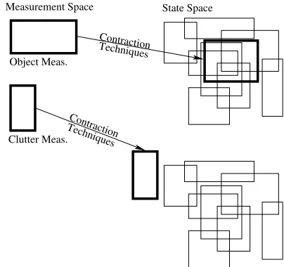
State Space

Contraction Techniques

Clutter Meas. Object Meas.

[image:6.612.335.537.53.243.2]

Contraction Techniques Measurement Space

Fig. 1: Illustration of the consistency between a set of box particles and object or clutter measurents.

clustering algorithm results in 3 clusters, each indexing 5 of the measurements, the number of weighted box particles after the update per predicted box particle is reduced from over 1 billion to 830 584. Although this reduces the number of weighted boxes by orders of magnitude for each box particle, this still results in a large computational burden.

D. Box Particle Filter Likelihood for Multiple Extended Ob-jects with Clustering and the Relaxed Intersection

The second cause for the large number of boxes is the uncertainty in which measurements are emitted by an object or are clutter. Using an interval based approach, it is possible to reduce the number of boxes due to this uncertainty.

The weight of each term in the posterior state pdf describes how likely the associations are, given the measurements. As observed in equation (21), each term is non-zero on the predicted state interval contracted by all the assigned object measurements. This interval is equivalent to the intersection of the contraction results for each of the measurements assigned as object originated. Each term can have clutter measurements assigned as object measurements. However, the contraction due to a clutter measurement can be an interval which does not exist, or is disjoint with the contracted intervals from the object originated measurements, as illustrated in Fig. 1. Since the overall result is dependent on the intersection, even a single clutter measurement assigned as an object measurement may result in the corresponding term having a zero weight. The computation of these terms can be avoided by approximating the intersection with the relaxed intersection. The relaxed in-tersection, first introduced in [34], corresponds to the classical intersection between intervals with the exception that it is allowed to relax a certain number of intervals in order to avoid an empty intersection.

(7)

approxima-tion for the posterior state pdf is obtained,

p(s_k_|Z_1:_k₎_≈

N

X

p=1

w_k(p₋₁) e−Pi∈I(p)λT ,i αkMk!

|I(p)|d X

n=1

|[sa,(p,n)

k ]|ρ Mk−u(p)

|[s(p)

k|k−1]|

U_[_sa,(p,n)

k ]

(s_k₎

u(p)

Y

ℓ=1

λT ,(b_n)ℓp(z

(a)ℓ

k |[x

(p) (b_n₎_ℓ,k])

, (24)

whereu(p)_{is the number of consistent intervals which results}

in a non-empty relaxed intersection. In order to determine the contracted state, [sa_k,(p,n)], the sub-states of each object are considered individually. The index for all the measurements assigned to object i, according to clustering, is defined by the set B. Since only these measurements contract the sub-state of object i, the resulting contraction result for all mea-surements is given by [xa_i,k,(p,n)] =

{|B|−u(p)i }

T ℓ∈B [x

ℓ,(p,n)

i,k ] with

u(p)₌P i∈I(p)u

(p)

i .

Considering the same example of 3 objects and 15 measure-ments, if the clustering algorithm results in 3 clusters, each indexing 5 of the measurements, the number of weighted box particles after the update per predicted box particle is reduced from 830 584 with the approximate posterior in equation (23) to 27 with the approximate posterior in equation (24).

Two issues remain with the calculation of the approximate pdf in equation (24). Firstly, the relaxed intersection does not explicitly indicate the indices of the u measurements which result in the non-zero intersection, which means it is not possible to evaluate the corresponding measurement likelihood for a single object expressions. Secondly, it is required to ensure that the box particle weight is represented by a single scalar value. If the measurement likelihood for a single object could be evaluated, this result may not be the case. Several approaches could be used to overcome this, such as selecting the midpoint of the box particle for measurement likelihood for a single object evaluation. The approach adopted in this paper overcomes both remaining issues by approximating the measurement likelihood for a single object with a uniform distribution, as done previously in [1],

p(zj_k|xi,k)≈Ur(x_i,k₎(zj_k). (25)

wherer(xi,k)represents the region in the measurement space where measurements from object i may exist, based on the model of object i, and sensor noise characteristics. This approximation is valid if the uncertainty in the sensor error is significantly smaller than the extent of the object. In sum-mary, the posterior at the previous time step,p(sk−1|Z1:k−1),

is approximated by {w_k(p₋)₁,[s(_kp₋)₁]}N

p=1, and the posterior

at the current time step, p(sk|Z1:k) is approximated by {{w(_kp,n),[s(_kp,n)]}N

p=1}

|I(p)_|d

n=1 , where[s (p,n)

k ] = [s a,(p,n)

k ], and

w(_kp,n)=w

(p)

k−1e −P

i∈I(p)λT ,i_|_[sa,(p,n)

k ]|ρ Mk−u(p)

|[s(p)

k|k−1]|

×

Y

ℓ∈I(p)

λT ,ℓ

|[r(x_ℓ,k_)]_|

uℓ . (26)

E. Box Particle Filter Resampling

The number of box particles representing the posterior state pdf grows randomly with each time step. The increase in the number of box particles is curbed through the implementation of a resampling step. The number of resampled particles is equal to the original number of box particles. In addition, the resampling step also relieves particle degeneracy [7]. The resampling step in the Box PF differs from the resampling step of the generic PF [25]. The resampling step in the Box PF is performed by a division of box particles [32] (a box particle selectedntimes during resampling is partitioned into

ndisjoint smaller boxes) or by other techniques.

A summary of the Box PF for multiple extended object tracking is given in Algorithm I.

Algorithm I. A Box Particle Filter for Multiple Extended Object Tracking

Initialization

Initialize the box particles based on the available prior information about the objects kinematic and parameter state.

RepeatforK time steps,k= 1, ...K, the following steps:

1) Prediction

Propagate the box particles through the state evolution model to obtain the predicted box particles. Apply interval inclusion functions as described in [35]. (The implementation presented in this paper is based on the INTLAB [36] toolbox, which contains a number of built-in routines for interval calculations.) 2) Measurement Update

a) Upon receiving the measurements, form intervals around them, taking into account the uncertainty of the sensor, thus obtaining the measurement likelihood boxes[Z_k_]_. b) Cluster the measurements to obtain the setCi, wherei∈

1, .., Nc.

c) Solve the CSP in Eq. (19) using the CP algorithm to obtain the contracted box particles for each measurement

[saℓ,(p,n)

k ].

d) Determine the combined contracted box particle,

[sa,(p,n)

k ], and the number of consistent intervals, u,

through the calculation of the relaxed intersection. e) Generate the set of weighted box particles according to

equation(26). 3) Output

Obtain a box estimate for the state of the extended objects based on the maximum box particle weight:

[ˆs_k_{] = arg max}_p₍s_k_|Z_k₎_≈_{arg max}

s_k w

(p,n)

k (27)

and a point estimateˆs_k _{for the extended shape based on the} center of the box estimate.

4) Resampling

ResampleN particles with high weights by division. Finally, reset the weights:w(_kp)= 1/N.

IV. PERFORMANCEEVALUATION

A. Testing Environment

(8)

-2 -1 0 1 2

x (m)

-6 -5 -4 -3 -2 -1 0 1

y (m)

(a) The three laser scanner devices are indicated with crossed boxes. Several mea-surements from the sensor lo-cated at the top left of the figure are displayed in red.

-2 -1 0 1 2

x (m) -6

-5 -4 -3 -2 -1 0 1

y (m)

Person 1 Person 2 Person 3

[image:8.612.65.294.51.242.2]

(b) Trajectories of the people moving through the corridor for the experiment.

Fig. 2: Layout of the corridor for the experiments.

Germany). The data is from a prototype security system developed by an EU funded project, representing an airport corridor. This data consists of range and bearing components obtained by three laser rangefinder devices. The measurement devices are positioned at three key locations in a curved corridor (see Fig. 2a). The considered scenario consists of three people who enter and traverse the corridor while being observed by the sensors. The trajectories of the people are shown in Fig. 2b.

Throughout their motion, each person moves in and out of the area visible by the sensors at different times. The sensors are positioned on the wall at the level of height of the hip.

B. Person Modeling

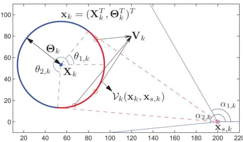
The HAMLeT test environment focuses on tracking mul-tiple people. Each person is modelled as an extended ob-ject in a two dimensional plane with a circular extent, as in Fig. 3. The sub-states of the state vector correspond-ing to the kinematics of each extended object is a vector,

Xi,k = (xci,k,x˙ci,k, yci,k,y˙ci,k)⊤, which comprises of the po-sition coordinates, xc

i,k, yci,k, and respective velocity compo-nents, x˙c

i,k,y˙i,kc . In this scenario the subset of states of the state vector that comprises the parameters used to model the extent of each object reduces to a scalar representing the radius of the circle used to approximate the extent,Θi,k=Ri,k.

In this paper the nearly constant velocity motion model [38] is representing the motion of each person, in two dimensions

Xi,k=AXi,k−1+ΓηX, (28)

where A = diag(A1,A1), A1 =

1 Ts

0 1

, Γ ₌

T2

s/2 Ts 0 0

0 0 T2

s/2 Ts ⊤

[image:8.612.313.560.53.198.2]

,Tsis the sampling interval and

Fig. 3: Notations and definitions for a single circular extended object.

ηX ∼ N(0,QX)is the system dynamics noise, with covari-ance matrixQX. It is assumed thatQX=diag(Q1σx2,Q1σ2y), whereQ1=

T4

s/4 Ts3/2

T3

s/2 Ts2

andσxandσy are the accel-eration noise standard deviations for the xandy coordinate, respectively. The evolution model for the extent parameter is

Θi,k= Θi,k−1+ηΘ, (29)

where ηΘ ∼ N(0, σR2). The visible border for a circular extended object is described as follows

Vk(xi,k,xs,k) = (xci,k+Ri,kcos(θk), yi,kc +Ri,ksin(θk)), (30)

whereθk∈[θ1,k, θ2,k], with thejth point source defined as,

Vj

i,k= (x c

i,k+Ri,kcos(θj_k), yi,kc +Ri,ksin(θj_k)). (31)

A graphical representation is shown on Fig. 3. The measure-ment zj_k collected from a sensor is in polar coordinates and consists of rangedj_kand bearingβj_k. The observation equation is thus given by

zj_k= (dj_k, β_kj)⊤=h(Vj_i,k) +wj_k, (32)

whereh(·)is

h(Vj

i,k) =

  

q

(xc

i,k+Ri,kcos(θ j

k)−xs,k)2+(y c

i,k+Ri,ksin(θ j

k)−ys,k)2

tan−1

yc

i,k+Ri,ksin(θkj)−ys,k

xc

i,k+Ri,kcos(θjk)−xs,k

  .

(33)

The measurement noisewj_k = (w_d,kj , wj_β,k)⊤_{, is zero mean} Gaussian, with a known covariance matrixΣ₌_diag₍_σ2

(9)

Algorithm II. Solving the CSP For Circular Extended Object Tracking

1) Transform the range and bearing measurements into the x-y

plane using an inclusion function:

h

z1j

i

= [Cz1]

h

djk

i

,hβkj

i , h zj 2 i

= [Cz2]

h

dj k

i

,hβj k

i

, (34)

where[zj

1]and[z

j

2]represent thexandydimension converted box measurements respectively, and [Cz1](·) and [Cz2](·)

represent the corresponding inclusion functions.

2) Perform contraction on the sub-states corresponding to each object for each particle and measurement based on the follow-ing equations

R(p)_k

=

R(p)_k

∩   s h

z₁j

i −

x(p)_c,k

2 +

h

zj₂

i −

y(p)_c,k

2 , (35)

x(p)_c,k

=

x(p)_c,k

∩



 h

z₁ji± s

R(p)_k

₂ −

h

z₂ji−

y_c,k(p)

₂ 

,

˙ x(p)_c,k

=

˙ x(p)_c,k

∩    

x(p)_c,k

−

x(p)_c,k

−1 Ts     ,

y_c,k(p)

=

y(p)_c,k

∩



 h

zj₂i± s

R(p)_k

₂ −

h

zj₁i−

x(p)_c,k

₂ 

,

˙ y_c,k(p)

=

˙ y(p)_c,k

∩    

y_c,k(p)

−

y(p)_c,k

−1 Ts     ,

z(p)_1,j

=hzj₁i∩ 



x(p)_c,k

±

s

R(p)_k

₂ −

h

z₂ji−

y_c,k(p)

₂ 

,

z(p)_2,j

=hzj₂i∩ 



x(p)_c,k

±

s

R(p)_k

2

−

z(p)_1,j

−

x(p)_c,k

2

.

3) Contract the original measurements with the contracted con-verted measurements:

h

d(_kp),ji=hdj_ki∩

Cz−11

h

z(₁p,j)

i

,hz₂(p,j)

i

,

h

βk(p),j

i

=hβkj

i

∩

Cz−12

h

z₁(p,j)

i

,hz₂(p,j)

i

,

(36)

4) Repeat steps 2) and 3) sequentially until the gain in amount of contraction is sufficiently small. The amount of contraction could be checked or the steps could be iterated a fixed amount of times.

C. Performance Comparison

The algorithms’ evaluation is performed on a mobile com-puter with Intel(R) Core(TM) i7-4702HQ CPU @ 2.20GHz and with 16 GB of RAM. A comparison is made between the performance of the Box PF, a state-of-the-art PF, here after referred to as the border parameterized (BP) PF, and the output of a purely clustering approach. The BP PF is the extended object tracking PF presented in [30] adapted for a varying number of extended objects, further details can be found in Appendix A. Clustering is performed with the DBSCAN algorithm [39]. This is a density based clustering algorithm which groups the measurements that are closely packed together into a single cluster. DBCSAN is well suited to the problem of interest as it does not require knowledge of the number of clusters, and the density of the measurements from each object is consistent. The centroid of an object is estimated as the mean of all measurements assigned as a cluster. The radius of an object is approximated as the maximal distance between the centroid and any measurement assigned

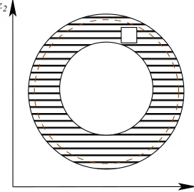
z₂

[image:9.612.369.505.56.191.2]

z₁

Fig. 4: The contraction of a box particle illustrated by a single measurement for a circular extended object. The square box represents a measurement. The filled circular region represents the projection of a box particle sub-states for a single object to the measurement space. The dotted line illustrates the reduction in the interval shape due to contraction by the measurement.

to the cluster. A threshold variable was introduced to reduce the effects of clutter. The results are averaged over a total of 100 independent runs where the measurements are perturbed by the measurement noise for each run. The performance is evaluated based on the Optimal Sub-Pattern Assignment (OSPA) [40] for the position of the objects, cardinality for the existent variables, the statistics of the existent object extents, and the average simulation time.

D. Filter Parameters and initialization

The Box PF utilizes the output of the DBSCAN algorithm. DBSCAN requires two parameters, ǫ = 0.43, related to the density of the clusters, and the minimum number of points required to form a dense region, which is selected as 1. In this simulation the regionr(xi,k)is represented by equation (31). The other parameters used in simulation for the performance evaluation are as follow: σx = 0.05m/s2, σy = 0.05m/s2,

σR = 0.05m, σd = 0.025m, σβ = 0.1π/180rad, Ts = 1s,

λT = 50,ρ= 1×10−4, Pe= 0.9, F = 30.

The filters utilize a uniform distribution to initialize each object sub-state when an object birth occurs. In the case of the Box PF, the same uniform region where the BP PF randomly generate particles from is subdivided so that the entire region is encompassed by all the box particles. This region, for each object sub-state, is located at the entrance/exit of the corridor: [xc] = [−1.5,−0.5]∪[0.5,1.5] m, [ ˙xc] = [−0.1,0.1] m/s, [yc] = [−1,0]m, [ ˙yc] = [−0.1,0.1]m/s,[R] = [0,0.3]m.

E. Results

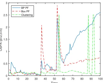
The performance of the filters is examined for 3 cases: a small, medium, and large number of particles. The average OSPA results for each case are illustrated in Fig. 5 to 7. The spikes in the results correspond to a mismatch in cardinality.

(10)

0 10 20 30 40 50 60 70 80 90 100

Time

0 0.5 1 1.5 2 2.5 3

OSPA (p=2,c=5)

[image:10.612.347.528.52.196.2]

BP PF Box PF Clustering

Fig. 5: Comparison of the average OSPA for the BP PF with 5000 particles, the Box PF with 32 particles, and DBSCAN clustering.

0 10 20 30 40 50 60 70 80 90 100

Time

0 0.5 1 1.5 2 2.5 3

OSPA (p=2,c=5)

[image:10.612.84.265.69.214.2]

0 10 20 30 40 50 60 70 80 90 100

Time

0 0.5 1 1.5 2 2.5 3

OSPA (p=2,c=5)

0 10 20 30 40 50 60 70 80 90 100

Time 1

1.5 2 2.5 3 3.5 4

Cardinality

[image:10.612.346.527.258.404.2]

Ground Truth BP PF Box PF Clustering

Fig. 8: Comparison of the average cardinality for the BP PF with 5000 particles, the Box PF with 32 particles, and DBSCAN clustering.

0 10 20 30 40 50 60 70 80 90 100

Time 1

1.5 2 2.5 3 3.5 4

Cardinality

[image:10.612.84.266.302.452.2]

from the objects when they first enter the observable region of a sensor. In the case of the clustering algorithm, the spikes are caused by poorly selected parameters in the clustering algorithm. This highlights the robustness of the Box PF to the selection of parameters for the clustering algorithm. When cardinality errors are not present, the clustering algorithm performs on par with the filtering approaches with respect to OSPA. This is aligned with the findings in [41], [42] where clustering algorithms are applied in the context of object tracking. In the case of the filters, decreasing the number of particles increases the amount of error, however, it is worth noting that a decrease in the number of particles for the BP PF also causes the filter to become unstable when three objects are within the scene. The average cardinality results for each case are illustrated in Figs. 8 to 10. The cardinality of the Box PF is significantly more robust to different numbers of box particles and clustering parameters.

[image:10.612.84.266.537.683.2]

(11)

0 10 20 30 40 50 60 70 80 90 100 Time

1 1.5 2 2.5 3 3.5 4

Cardinality

[image:11.612.51.232.52.198.2]

[image:11.612.87.263.278.364.2]

TABLE I: Existent object extent statistics.

Algorithm N Mean (m) Standard Deviation (m)

Box PF

4 0.23 0.03

16 0.21 0.04

32 0.2 0.05

BP PF

1000 0.24 0.13

2500 0.23 0.13

5000 0.21 0.11

Clustering 0.3 0.07

The rudimentary approach of approximating the extent in the clustering approach leads to an over estimate of the extent which is sensitive to clutter.

The computational time for each of the considered cases under the same conditions is given in Table II. Note that implementing the Box PF with the INTLAB [36] MATLAB toolbox is just one possible way. This toolbox was initially designed and optimized for estimating rounding errors. Faster realizations of the Box PF in C/C++ are also possible. For instance, in [43] the Box Probability Hypothesis Density Filter is shown to be 10.9 times faster than the Probability Hypothesis Density Filter working with point particles (both implemented in C++). Further optimization is possible for the Box PF realization, thus the results in Table II would represent a minimum efficiency improvement. The Box PF is also a very attractive solution from the perspective of distributed estimation, as shown in [44]. The clustering approach offers significant computational savings, but this comes at a cost of reduced estimation accuracy of the objects’ extents which are

TABLE II: Average Matlab computational time comparison.

Algorithm N Computation Time (s)

Box PF

4 43.38

16 118.56

32 282.24

BP PF

1000 67.68

2500 168.53

5000 417.66

Clustering 4.25

sensitive to clutter.

An attractive benefit of the Box PF, not clearly illustrated in the results presented so far, is the ability of the filter to handle large regions of initial uncertainty. For example, the prior distribution on the sub-states related to the velocity components of each object is a uniform distribution with the following region of support: [−0.1,0.1]. This region caters for objects moving in any direction and was sufficient for the objects in the examined scenario, but when the magnitude is increased, the BP PF is unable to lock on to new born objects. This is due to the fact that the velocity of the object is not directly observed, causing the filter to diverge. However, due to contraction and the division of boxes in the resampling step, the Box PF is capable of handling larger regions of uncertainty. As an example, increasing the region to[−1,1], caused the BP PF to diverge in all three cases, where the Box PF performance was unaffected. This issue can be resolved by the BP PF by utilizing a larger number of particles, but this comes at the cost of an even greater computational complexity. In addition, filtering approaches have track continuity when the detection probability is low.

V. CONCLUSIONS

This paper presents a Box PF method for multiple extended object tracking. The approach is especially suitable to practical tasks where the sensor error characteristics are not exactly known, but instead the regions to which they belong are available. A theoretical derivation of the generalized likelihood function of the Box PF is presented for the case when the measurements contain clutter noise. The proved equation is further modified to minimize the computational complexity. It is shown that the Box PF can work efficiently with four to thirty two box particles, whereas the particle filter working with point particles needs hundreds and thousands of particles to achieve the same accuracy. The Box PF has been shown to have several advantages when compared to the BP PF. This includes a significant computational gain, more than 32%, which could potentially be further exploited through an implementation on a platform that is efficient in interval arithmetic. Compared with the standard PF the Box PF exhibits robustness for a significantly smaller number of box particles which completely encompass the initialization region. The performance of the method is validated with real data from laser rangefinder sensors.

Future work will focus on the expansion and validation of the method for more general application settings, such as asynchronous multirate sensor networks [45], and correlated sensor noise [46].

Acknowledgments. We are grateful to the support from

[image:11.612.95.256.665.742.2]

(12)

no. 688082. We thank the anonymous reviewers and the Associate Editor for their constructive suggestions.

APPENDIX

A. Border Parameterized Particle Filter

In [30] a PF for tracking multiple extended objects is pre-sented. However, in this case the number of extended objects is fixed and known. This algorithm has been adapted to consider a varying number of extended objects as in Section II-A. With respect to the notation developed in Section II-B, the BP PF represents the posterior state pdf with the following discrete approximation

p(sk|Z1:k) = N X

p=1

w(_kp)δsk−s(_kp)

, (37)

where δ(·) is the Dirac delta function, and the weights, {w(_kp)}N

p=1, are normalized so that

P pw

(p)

k = 1.

The transition pdf, described in (4), is used to modify the set of particles, represented by {s(_kp_|_k)₋₁}N

p=1.The weight of each

particle is re-evaluated based on the latest set of measurements and the generalized likelihood function of (6).

Since the measurement likelihood for a single object,

p(zj_k|xi,k), is analytically intractable, a Monte Carlo method is used to approximate it, as in [17] and [47]. For each particle existent object subspace, x(_i,kp)_|_k₋₁, the sup-port of p(Vj_i,k|x_i,k(p)_|_k₋₁) is defined by a uniform distribu-tion over the angular range [θ1,k, θ2,k] of the visible border Vk(x(_i,kp)_|_k₋₁,xs,k)with respect to the object center. A sampled point source can be obtained by first sampling from:

n

θ_k(b,f)

oN,F

b=1,f=1∼ U[θ1,k,θ2,k](θk)

, (38)

followed by the substitution of nθ(_kb,f)oN,F

b=1,f=1 into (31),

resulting in a random set of samples denoted as Jk = n

Vj,_i,k(b,f)o

N, F

b=1,f=1, where F is the number of samples from

the object border. The Monte Carlo approximation for the measurement likelihood of a single object is then given by:

p(zj_k|x(_i,kp)_|_k₋₁) =

Z

p(zj_k|Vj_i,k)p(Vj_i,k|x(_i,kp)_|_k₋₁)dVj_i,k,

≈ 1

F

X

Vj

i,k∈Jk

p(zj_k|Vj_i,k). (39)

The BP PF is summarized in Algorithm III.

B. Expanded Generalized Likelihood Proof

According to equation (15), given I, for any value ofMk:

Mk

Y

m=1

ρ+X i∈I

λT ,ip(zmk|xi,k)

=ρMk₊

Mk

X

m=1

(Mk m)

X

j=1 |I|m

X

n=1

ρMk−m_×

m

Y

ℓ=1

(a_m,j₎_ℓ

k |x(b_m,n₎_ℓ,k).

(40)

Algorithm III. The Border Parameterized Particle Filter for Multiple Extended Object Tracking

Initialization

k = 0, Initialize the set of particles based on the available prior information,{s(p)

0 ∼ p(s0)}. Set initial weights{w0(p)}Np=1= N1. Repeatthe following steps forT time steps,k= 1, ...T:

1) Prediction

Propagate the particles,{s(p)

k−1}

N

p=1with the state transition pdf (equation(4)) to obtain the predicted particles,{s(p)

k|k−1}

N p=1. 2) Measurement Update

On the receipt of a new measurement:

a) Evaluate the measurement likelihood for a single object,

p(zj

k|x

(p)

i,k|k−1), according to(39) for all the measure-ments.

b) Calculate the weights w_k(p), p = 1, ..., N using terms from step 2-a) and equation(6).

3) Output

Calculate the estimated state vectorˆs_k_{based on the maximum} particle weight:

ˆ

s_k_{= arg max}_p₍s_k_|Z_k₎_≈_{arg max}

s_k w

(p)

k (41)

4) Resampling

a) Compute the effective sample size Nef f=

1

PN p=1

ˆ

w_k(p)2

b) Selection

IfNef f≤Nthresh (with e.g.Nthresh= 2N/3)

resam-ple the particles. Finally, reset the weights:w(kp)= 1/N.

To simplify notations, define: cm,i = p(zmk |xi,k) and C(c1,I, c2,I, ..., cMk,I;ψ) represents the summation of all ψ unique combinations of cm,i terms multiplied by the associated object densities, with C(c1,I, c2,I, ..., cMk,I; 0) = 1, C(c1,I, c2,I, ..., cMk,I;−1) = 0, and C(c1,I, c2,I, ..., cMk,I;Mk + 1) = 0. For example, if I = {1,2}, then C(c1,I, c2,I, c3,I; 2) =

λ2

T ,1c1,1c2,1 + λT ,1λT ,2c1,1c2,2 + λT ,1λT ,2c1,2c2,1 + λ2

T ,2c1,2c2,2 + λ2_{T ,}1c2,1c3,1 + λT ,1λT ,2c2,1c3,2 + λT ,1λT ,2c2,2c3,1 + λ2T ,2c2,2c3,2 + λ2T ,1c1,1c3,1 + λT ,1λT ,2c1,1c3,2 + λT ,1λT ,2c1,2c3,1 + λ2T ,2c1,2c3,2. A

useful decomposition of the expression in this form is: C(c1,I, c2,I, ..., cMk+1,I;ψ) = C(c1,I, c2,I, ..., cMk,I;ψ) +

P

i∈IλT ,icMk+1,iC(c1,I, c2,I, ..., cMk,I;ψ−1). The compact form of equation (40) is

Mk

Y

m=1

ρ+X i∈I

λT ,icm,i

!

= Mk

X

m=0

ρMk−m_C₍_c

1,I, c2,I, ..., cMk,I;m).

(42) Base case: Mk = 1:

ρ+X i∈I

λT ,ic1,i=

1

X

m=0

ρ1−m_C₍_c

1,I;m)

=ρ1−0C(c1,I; 0) +ρ1−1C(c1,I; 1)

=ρ+X

i∈I

λT ,ic1,i. (43)

Inductive hypothesis: Suppose equation (42) holds for all values of Mk.

(13)

measure-ments,

Mk+1

Y

m=1

ρ+X

i∈I λT ,icm,i

=



 Mk

Y

m=1



ρ+ X

i∈I λT ,icm,i



 

 

ρ+ X

i∈I

λT ,icMk+1,i





=

Mk

X

m=0

ρMk−mC(c1,I, c2,I, ..., cMk,I;m)×



ρ+ X

i∈I

λT ,icMk+1,i





=

Mk+1

X

m=0

ρMk+1−mC₍c1,I, c2,I, ..., cMk,I;m)

+X

i∈I

λT ,icMk+1,i

Mk+1

X

m=0

ρMk+1−m×

C(c1,I, c2,I, ..., cMk,I;m−1)

=

Mk+1

X

m=0

ρMk+1−m

C₍c1,I, c2,I, ..., cMk,I;m)

+X

i∈I

λT ,icMk+1,iC(c1,I, c2,I, ..., cMk,I;m−1)

=

Mk+1

X

m=0

ρMk+1−mC(c1,I, c2,I, ..., cMk+1,I;m). (44)

By the principle of mathematical induction, the proposition holds for all Mk ∈N.

REFERENCES

[1] A. De Freitas, L. Mihaylova, A. Gning, D. Angelova, and V. Kadirka-manathan, “Autonomous Crowds Tracking with Box Particle Filtering and Convolution Particle Filtering,”Automatica, vol. 69, pp. 380–394, 2016.

[2] M. Feldmann and W. Koch, “Road-map Assisted Convoy Track Main-tenance using Random Matrices,” inProc. of 11th Int. Conf. on Infor-mation Fusion, June 2008, pp. 1–8.

[3] D. Angelova and L. Mihaylova, “Extended Object Tracking Using Monte Carlo Methods,”IEEE Trans. on Signal Processing, vol. 56, no. 2, pp. 825–832, Feb 2008.

[4] A. Carmi, F. Septier, and S. J. Godsill, “The Gaussian Mixture MCMC Particle Algorithm for Dynamic Cluster Tracking,”Automatica, vol. 48, no. 10, pp. 2454 – 2467, 2012.

[5] K. Granstr¨om, C. Lundquist, and U. Orguner, “Tracking Rectangular and Elliptical Extended Targets using Laser Measurements,” inProc. of 14th Int. Conf. on Information Fusion, July 2011, pp. 1–8.

[6] F. Septier, S. K. Pang, A. Carmi, and S. Godsill, “On MCMC-Based Particle Methods for Bayesian Filtering: Application to Multitarget Tracking,” in Proc. of the IEEE Int. Workshop on Computational Advances in Multi-Sensor Adaptive Processing, Dec. 2009, pp. 360– 363.

[7] L. Mihaylova, A. Carmi, F. Septier, A. Gning, S. Pang, and S. Godsill, “Overview of Bayesian Sequential Monte Carlo Methods for Group and Extended Object Tracking,”Digital Signal Processing: A Review Journal, vol. 25, no. 1, pp. 1–16, 2014.

[8] K. Granstr¨om and M. Baum, “Extended Object Tracking: Introduction, Overview and Applications,” 2016, arXiv preprint arXiv:1604.00970. [9] R. P. S. Mahler, “PHD Filters for Nonstandard Targets, I: Extended

Targets,”Proc. of 12th Int. Conf. on Information Fusion, pp. 915–921, 2009.

[10] K. Granstr¨om and U. Orguner, “A PHD Filter for Tracking Multiple Extended Targets Using Random Matrices,” IEEE Trans. on Signal Processing, vol. 60, no. 11, pp. 5657–5671, Nov 2012.

[11] C. Lundquist, K. Granstr¨om, and U. Orguner, “An Extended Target CPHD Filter and a Gamma Gaussian Inverse Wishart Implementation,”

IEEE Journal of Selected Topics in Signal Processing, vol. 7, no. 3, pp. 472–483, June 2013.

[12] M. Beard, S. Reuter, K. Granstr¨om, B. T. Vo, B. N. Vo, and A. Scheel, “Multiple Extended Target Tracking With Labeled Random Finite Sets,”

IEEE Transactions on Signal Processing, vol. 64, no. 7, pp. 1638–1653, April 2016.

[13] M. Baum and U. Hanebeck, “Shape Tracking of Extended Objects and Group Targets with Star-convex RHMs,” inProc. of 14th Int. Conf. on Information Fusion, 2011.

[14] M. Baum and U. D. Hanebeck, “Extended Object Tracking Based on Set-Theoretic and Stochastic Fusion,” IEEE Trans. on Aerospace and Electronic Systems, vol. 48, no. 4, pp. 3103–3115, Oct. 2012. [15] J. Lan and X. Li, “Tracking of Maneuvering Non-Ellipsoidal Extended

Object or Target Group Using Random Matrix,”IEEE Trans. on Signal Processing, vol. 62, no. 9, pp. 2450–2463, May 2014.

[16] K. Gilholm and D. Salmond, “Spatial Distribution Model for Tracking Extended Objects,”IEE Proc. Radar, Sonar and Navigation, vol. 152, no. 5, pp. 364–371, Oct. 2005.

[17] Y. Boers, H. Driessen, J. Torstensson, M. Trieb, R. Karlsson, and F. Gustafsson, “Track-before-detect Algorithm for Tracking Extended Targets,”IEE Proc. Radar, Sonar and Navigation, vol. 153, no. 4, pp. 345–351, Aug. 2006.

[18] J. Koch, “Bayesian Approach to Extended Object and Cluster Tracking using Random Matrices,” IEEE Trans. on Aerospace and Electronic Systems, vol. 44, no. 3, pp. 1042–1059, July 2008.

[19] M. Baum and U. D. Hanebeck, “Extended Object Tracking with Ran-dom Hypersurface Models,”IEEE Trans. on Aerospace and Electronic Systems, vol. 50, no. 1, pp. 149–159, Jan. 2014.

[20] N. Wahlstr¨om and E. ¨Ozkan, “Extended Target Tracking Using Gaussian Processes,”IEEE Trans. on Signal Processing, vol. 63, no. 16, pp. 4165– 4178, Aug. 2015.

[21] F. Abdallah, A. Gning, and P. Bonnifait, “Box Particle Filtering for Non-linear State Estimation using Interval Analysis ,”Automatica, vol. 44, no. 3, pp. 807 – 815, March 2008.

[22] N. Merlinge, J. Marzat, and L. Reboul, “Optimal guidance and observer design for target tracking using bearing-only measurements,” ONERA, France, Tech. Rep., 2016.

[23] N. Merlinge, K. Dahla, and H. Piet-Lahanier, “A Box Regularized Parti-cle Filter for terrain navigation with highly non-linear measurements,” in

Proc. of the 20th IFAC Symposium on Automatic Control in Aerospace (ACA), vol. 49, no. 17, 2016, pp. 361–366.

[24] A. Gning, L. Mihaylova, and F. Abdallah, “Mixture of Uniform Proba-bility Density Functions for Nonlinear State Estimation Using Interval Analysis,” inProc. of 13th Int. Conf. on Information Fusion, 2010, pp. 1–8.

[25] A. Gning, L. Mihaylova, F. Abdallah, and B. Ristic, “Particle Filtering Combined with Interval Methods for Tracking Applications,” in Inte-grated Tracking, Classification, and Sensor Management: Theory and Applications, M. Mallick, V. Krishnamurthy, and B.-N. Vo, Eds. John Wiley & Sons, New Jersey, USA, 2012, pp. 43–74.

[26] N. Petrov, M. Ulmke, L. Mihaylova, A. Gning, M. Schikora, M. Wieneke, and W. Koch, “On the Performance of the Box Particle Filter for Extended Object Tracking Using Laser Data,” inWorkshop on Sensor Data Fusion, Sept. 2012, pp. 19 –24.

[27] N. Petrov, A. Gning, L. Mihaylova, and D. Angelova, “Box Particle Filtering for Extended Object Tracking,” inProc. of 15th Int. Conf. on Information Fusion, July 2012, pp. 82 – 89.

[28] J. Vermaak, N. Ikoma, and S. Godsill, “Sequential Monte Carlo Frame-work for Extended Object Tracking,” IEE Proc. Radar, Sonar and Navigation, vol. 152, no. 5, pp. 353–363, Oct. 2005.

[29] F. Septier, J. Cornebise, S. Godsill, and Y. Delignon, “A Comparative Study of Monte-Carlo Methods for Multitarget Tracking,” in IEEE Statistical Signal Processing Workshop, June 2011, pp. 205–208. [30] K. Gilholm, S. Godsill, S. Maskell, and D. Salmond, “Poisson Models

for Extended Target and Group Tracking,” inOptics & Photonics 2005, vol. 5913. International Society for Optics and Photonics, 2005. [31] A. Gning, B. Ristic, L. Mihaylova, and F. Abdallah, “An Introduction

to Box Particle Filtering [Lecture Notes],” IEEE Signal Processing Magazine, vol. 30, no. 4, pp. 166–171, July 2013.

[32] A. Gning, B. Ristic, and L. Mihaylova, “Bernoulli Particle/Box-Particle Filters for Detection and Tracking in the Presence of Triple Measurement Uncertainty,” IEEE Trans. on Signal Processing, vol. 60, no. 5, pp. 2138–2151, May 2012.

[33] L. Jaulin, M. Kieffer, O. Didrit, and E. Walter,Applied Interval Analysis. Springer-Verlag, 2001.