Experimental and numerical evaluation of single phase adiabatic flows in plain and enhanced microchannels

Rochester Institute of Technology

RIT Scholar Works

Theses Thesis/Dissertation Collections

11-1-2007

Experimental and numerical evaluation of single

phase adiabatic flows in plain and enhanced

microchannels

Follow this and additional works at:http://scholarworks.rit.edu/theses

This Thesis is brought to you for free and open access by the Thesis/Dissertation Collections at RIT Scholar Works. It has been accepted for inclusion in Theses by an authorized administrator of RIT Scholar Works. For more information, please [email protected].

Recommended Citation

Experimental and Numerical Evaluation of Single Phase Adiabatic

Flows in Plain and Enhanced Microchannels

by

AKHILESH V. BAPAT

A Thesis Submitted in Partial Fulfillment of the Requirements for the

MASTER OF SCIENCE IN

MECHANICAL ENGINEERING

Approved by:

Dr. Satish G. Kandlikar

Department of Mechanical Engineering (Thesis Advisor)

Dr. Jeffrey Kozak

Department of Mechanical Engineering

Dr. P. Venkataraman

Department of Mechanical Engineering

Dr. Edward C. Hensel

Department Head of Mechanical Engineering

DEPARTMENT OF MECHANICAL ENGINEERING ROCHESTER INSTITUTE OF TECHNOLOGY

THESIS REPRODUCTION PERMISSION STATEMENT

PERMISSION GRANTED

TITLE:

“Experimental and Numerical Evaluation of Single Phase Adiabatic Flows in Plain and Enhanced Microchannels”

I, Akhilesh V Bapat, hereby grant permission to the Wallace Library of the Rochester Institute of Technology to reproduce my dissertation in whole or in part. Any reproduction will not be for commercial use or profit.

ABSTRACT

Thermal Dissipation is a critical issue in the performance of semiconductor devices. The current practice is to use forced convection by air over a heat sink which is bonded to the microelectronic device. With increased packing density of the circuits inside a chip, large amounts of heat is generated and air cooling is no longer sufficient. Forced liquid convection using microchannels is considered to be a viable option for cooling of these microprocessor chips. This work deals with the evaluation of the single phase pressure drop in microchannels.

There are two types of microchannels under consideration. Plain microchannels which have basically long uninterrupted flow channels while the enhanced channels which have the interrupted flow lengths. Enhanced microchannels, because of their offset strip fin geometry, significantly increase both the heat transfer as well as the pressure drop. This work deals with the evaluation of single phase flow pressure drop in both plain and enhanced microchannels.

For plain microchannels there have been a few investigations in the literature which suggest that the microchannel performance can generally be predicted using the classical fluid flow equations. However there are some experiments that still show departure from the classical theory that cannot be explained. It is proposed in this work that the reason for this discrepancy can be traced to the effects due to flow maldistribution in plain microchannels. A systematic experimental investigation is performed to study the effects of slight variations in channel dimensions and their influence on the flow maldistribution in an attempt to validate the applicability of classical theory to microchannel flows. Enhanced microchannels however have not been investigated thoroughly. There is very few data available in the literature. FLUENT is a CFD software which can be used as a tool to design and optimize these enhanced channels. However it has to be first validated with experiments. Thus pressure drop experiments are carried out on an offset strip fin silicon microchannel and the data is predicted using FLUENT, which is CFD software. Also existing predictive models for friction factor in offset strip fin minichannels are tested to check their validity for microchannel flows.

For plain microchannels, it seen that with uniform flow assumption, the friction factor is either underpredicted or overpredicted using the theory depending upon the reference channel dimension. However by accounting flow maldistribution in plain microchannels, friction factor can be accurately determined using theoretical equations. For enhanced microchannels it is observed that FLUENT can predict the pressure drop within 10%.

TABLE OF CONTENTS

List of Figures ... vi

List of Tables ... viii

List of Symbols ... ix

1.0 INTRODUCTION ...1

1.1 Brief History of Microchannel Heat Sinks ...5

1.2 Thesis Outline ...6

2.0 LITERATURE REVIEW ...10

2.1 Plain Microchannels ...10

2.2 Enhanced Microchannels ...15

2.3 Objectives ...18

3.0 EXPERIMENTAL SETUP FOR PLAIN MICROCHANNELS ...20

3.1 Flow Loop ...21

3.2 Test Section Design ...22

3.3 Channel Dimensions ...24

3.4 Instrumentation and Data Acquisition ...25

3.5 Experimental Uncertainties ...26

3.6 Experimental Procedure ...27

4.0 EXPERIMENTAL SETUP FOR ENHANCED MICROCHANNELS ...28

4.1 Flow Loop ...28

4.2 Test Section Details ...30

5.0 NUMERICAL SETUP OF ENHANCED MICROCHANNELS ...33

5.1 Flow Geometry ...33

5.2 Zone Specifications ...37

5.3 Mesh Generation ...38

5.4 Mesh Quality ...39

5.5 Mesh Size Dependence ...41

6.0 MALDISTRIBUTION ANALYSIS FOR PLAIN MICROCHANNELS ...43

6.1 Estimating Flow Maldistribution ...43

6.2 Friction Factor Prediction ...46

7.0 ENHANCED MICROCHANNELS – FRICTION FACTOR ANALYSIS ...49

7.1 Enhanced Microchannel Data Reduction ...49

7.1.1 Experimental Friction Factor ...49

7.1.2 Numerical Friction Factor ...51

7.2 Enhanced Minichannel Correlation Data Reduction ...51

8.0 RESULTS ...54

8.1 Plain Channels ...54

8.2 Enhanced Channels ...64

8.2.1 Minichannel Correlation Validity for Existing Microchannel Data .64 8.2.2 CFD Results for Enhanced Microchannels ...69

9.0 CONCLUSIONS AND FUTURE WORK ...71

9.1 Conclusions ...71

REFERENCES ...74

LIST OF FIGURES

Figure 1.1: Schematic of Air Cooled Microprocessor, Steinke (2005) 2

Figure 1.2: Schematic of Flow in Plain Microchannels 3

Figure 1.3:Schematic of “Enhanced” Microchannels 4

Figure 1.4 (a): Flow Chart for Experimental Evaluation of Plain Microchannel Flows 7

Figure 1.4 (b): Flow Chart for Numerical Evaluation of Enhanced Microchannel Flows 8

Figure 2.1: Manifold images from side facing the channel and

channel chip, Colgan et al(2005) 17

Figure 3.1: Flow Loop for Investigation Single Phase Flows Plain Microchannel 21

Figure 3.2: Photograph of Copper Block Test Section with Parallel Microchannels 22

Figure3.3: Photograph of cover plate with inlet and outlet manifolds 23

Figure3.4: Assembly of the cover plate, test section and the insulating base 24

Figure 4.1: Schematic of the Flow Loop for Enhanced Microchannels 29

Figure 4.2: Enhanced Silicon Microchannel 30

Figure 4.3: Text Fixture Housing the Silicon Microchannel 31

Figure5.1: 1000X magnified image of offset strip fins from KEYENCE microscope 34

Figure5.2: Schematic of Unit Cell and Computational Domain 35

Figure5.3: Image of Unit Cell created in GAMBIT 36

Figure5.4: Meshed Unit Cell of Enhanced Channel 39

Figure 6.1: Schematic of multiple channels with inlet and outlet manifold configuration 42

Figure 8.1: Plot of dimensionless pressure drop

using maldistribution for channels 1(a) to 6(f) 56

Channel 1 (a) and 5(b) reference 58

Figure 8.3: Static Pressure Variation across the Centre Plane

Of The Unit Cell for Re 47 Flow 65

Figure 8.4: Inlet and Outlet Velocities for Re 162 66

Figure 8.5: Velocity Vector Plot Over the Fin at Re 162 67

Figure 8.6: Comparison of Experimental and Numerical Poiseuille Number 68

LIST OF TABLES

Table 1.1: Heat Transfer Coefficients for Forced Convection, Holman (1976) 1

Table 2.1: Summary of Investigation on Single Phase Flows In Microchannels 11

Table 3.1: Individual channel dimensional variability 24

Table 5.1: Mesh Size Sensitivity 41

Table 8.1: Estimated Channel Flow Rates and Measured Pressure Drop

for Plain Microchannels 55

LIST OF SYMBOLS

a channel width m

A area m2

b channel height m

Cp specific heat J kg-1 K-1

D diameter m

Dh hydraulic diameter m

f Fanning friction factor = ρ Δp Dh / 2 L G2

G mass flux kg m-2 s-1

k thermal conductivity W m-1 K-1

K loss coefficient

L channel length m

Lh hydrodynamic entrance length m

L+ non-dimensional entrance length

n number of channels

Pw wetted perimeter m

Re Reynolds number = G Dh / μ

s fin thickness m

x+ non-dimensional flow distance

x* non-dimensional thermal flow distance

Greek

αc microchannel aspect ratio = a / b

αc fin aspect ratio = s / b

Δ difference

μ viscosity N s m-2

ρ density kg m-3

Subscripts

app apparent

avg average b bulk or mean c cross section FD fully developed

i inlet

LMTD log mean temperature difference

m mean

o outlet

s surface

CHAPTER ONE

INTRODUCTION

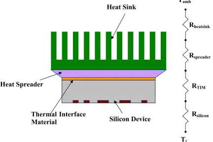
Thermal management of VLSI chips is very important. The reliability of these chips

decreases dramatically as the chip temperature increases beyond 110°C. Considering various

thermal resistance paths, it is customary to limit the temperature of the back side of an IC chip to

around 80 or 85 °C. The current industry practice employs a heat sink which is bonded to the

back side of the chip. A fan is placed on top of the heat sink which forces air through the

extended surface. Figure 1.1 shows a typical heat sink setup for cooling computer chips as

depicted by Steinke (2005). As shown in the fig. 1.1, the heat sink is typically made of copper or

aluminum. It is bonded using a Thermal Interface Material to the silicon device, to accommodate

for unequal thermal expansion. Heat Spreader is used to uniformly increase the heated surface

area for better uniform cooling. With the advances in microelectronic industry, the cooling

requirements are increasing and forced air cooling is no longer a viable option. Table 1.1 lists the

estimates of heat transfer coefficients for different mechanisms.

Table 1.1 Heat Transfer Coefficients for Forced Convection, Holman (1976)

HEAT TRANSFER MECHANISM h (W/m2_°C)

Forced Convection, Air ~100

Forced Convection, Water ~15000

T

Heat Sink

Fig. 1.1: Schematic of Air Cooled Microprocessor, Steinke (2005)

For cooling requirements in excess of 100 W/cm2, liquid cooling seems to be the right

solution. Heat transfer coefficients in the order of 100000 W/m2°C can be achieved with flow

boiling of water. However employing flow boiling also requires additional components like a

condenser. The overall cooling system gets very complicated and bulky. However it is possible

to achieve heat transfer coefficients more than 10000 W/m2°C with forced convection of water

by using microchannels as shown by Colgan et al. (2005). Jet impingement and evaporative

T

R

R

R

R

Heat Spreader

Thermal Interface

spray cooling are also attractive options which are considered for electronics chip cooling.

Microchannel performance is evaluated in this thesis.

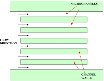
Microchannels have very small hydraulic diameters in the order of 200μm. Figure 1.2

shows a schematic of plain microchannels.

CHANNEL WALLS FLOW

DIRECTION

MICROCHANNELS

Fig. 1.2: Schematic of Flow in Plain Microchannels

The small flow cross sectional area associated with microchannels presents a large

surface area to the volume ratio which is responsible for increased heat transfer. This inherent

characteristic of microchannels enables them to be used for high heat flux cooling. The

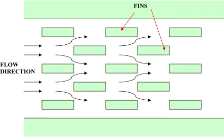
microchannels falls in the range of 10-200µm. Further increase in heat transfer can be achieved

by modifying the path of the flow of the fluid in the microchannels. The fin walls, which run

continuous along the flow length for plain channels, are periodically spaced and also offset.

Figure 1.3 shows the schematic of an enhanced microchannel which has a offset strip fin

configuration.

FLOW DIRECTION

FINS

Fig. 1.3: Schematic of an “Enhanced” Microchannel

Each new fin interrupts the flow and in the process there is a formation of boundary layer

is very high. This enables the offset strip fin microchannels to push the heat transfer coefficient

even higher than plain microchannels. However, the enhanced heat transfer also comes with

additional pressure drop. Pressure drop is increased because of boundary layer formation and

frictional form drag losses. This makes the hydraulic prediction of these channels very important.

Because of the complexity of the flow in these channels, it is very difficult for an analytical

solution. This work deals the evaluation of flows through both these configurations of

microchannels – plain and enhanced.

1.1 Brief History of Microchannel Heat Sink

The first concept for using microchannels as a heat exchanger device for VLSI circuits

was conceived by Tuckerman and Pease (1981). It was found that the microchannels are very

effective in heat dissipation. The reason for very high heat removal was associated with the fact

that microchannels have very small hydraulic diameters ranging to up to a few hundred microns.

This was in conjunction with the significant area enhancement due to the finned surface. Because

of smaller free flow areas, the power needed to pump fluid through smaller passages also

increased a lot. Thus increased pressure drop was a concern. Very high pressures required to

maintain the flow through these channels assured that microchannels predominantly operated in

the laminar regime. Although microchannels promised to be very effective, initially

microchannel research did not receive an impetus. Intel developed the 80286 microprocessor

which had significantly reduced the power consumption of the microelectronic device which

implied less waste heat.

By mid 90’s increased complexity and density of microelectronic circuits gave rise to

increase in the thermal dissipation requirements. Microchannel cooling was widely researched by

the academia and industry. Microchannels were a viable option for the practical implementation

conventional equations to predict the thermo-hydraulic performance of these microchannels.

There have been many papers in the literature with different views. Steinke and Kandlikar (2006)

carried out an exhaustive review of investigations dealing with microchannel cooling.

Other viable configurations which would utilize the potential of microchannels

investigated. It was found that the enhanced channels were the most promising for high heat flux

removal. These enhanced microchannels exhibit an interrupted fin design with the fins offset.

This causes periodic destruction of the boundary layer which accounts for very high values of

heat transfer coefficients. This type of configuration is widely used in the heat exchanger

applications like automotive cooling. Researchers have gathered data spanning over few decades

and come up with correlations to predict the pressure drop and heat transfer in offset strip fin

heat exchangers. However for offset strip finned microchannel no predictive models have been

developed.

The present work deals with the evaluation of single phase fluid flow in microchannels.

Both plain and enhanced microchannels have been investigated. The single phase predictions

would be evaluated for plain and enhanced channels.

1.2 Thesis Outline

This work deals with the experimental and numerical evaluation of single phase adiabatic

flows for both plain and enhanced microchannels. An outline is laid out in this section to

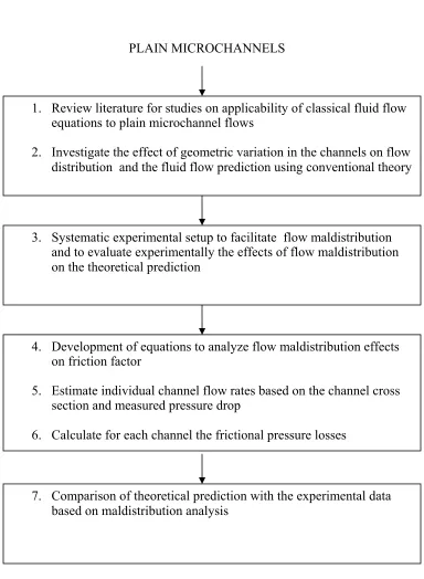
1. Review literature for studies on applicability of classical fluid flow equations to plain microchannel flows

2. Investigate the effect of geometric variation in the channels on flow distribution and the fluid flow prediction using conventional theory

3. Systematic experimental setup to facilitate flow maldistribution and to evaluate experimentally the effects of flow maldistribution on the theoretical prediction

7. Comparison of theoretical prediction with the experimental data based on maldistribution analysis

4. Development of equations to analyze flow maldistribution effects on friction factor

5. Estimate individual channel flow rates based on the channel cross section and measured pressure drop

6. Calculate for each channel the frictional pressure losses PLAIN MICROCHANNELS

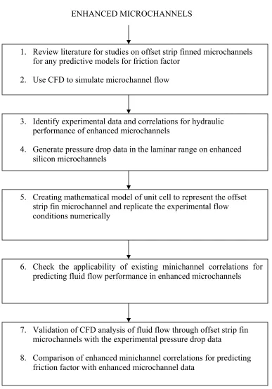
1. Review literature for studies on offset strip finned microchannels for any predictive models for friction factor

2. Use CFD to simulate microchannel flow

3. Identify experimental data and correlations for hydraulic performance of enhanced microchannels

4. Generate pressure drop data in the laminar range on enhanced silicon microchannels

6. Check the applicability of existing minichannel correlations for predicting fluid flow performance in enhanced microchannels

5. Creating mathematical model of unit cell to represent the offset strip fin microchannel and replicate the experimental flow conditions numerically

ENHANCED MICROCHANNELS

7. Validation of CFD analysis of fluid flow through offset strip fin microchannels with the experimental pressure drop data

8. Comparison of enhanced minichannel correlations for predicting friction factor with enhanced microchannel data

Figure 1.4 (a) shows the outline for the experimental evaluation of flows in plain

channels. Plain channels have been extensively investigated in the literature. A brief review is

conducted in Chapter Two. However there exist a lot of contradictory views about the validity of

classical fluid flow equations to the microchannel flow. It is seen that the conventional theory

either over predicts or underpredicts the microchannel pressure drops. These predictions are

based on equal flow distribution. Flow maldistribution introduced due to slight geometric

variation is thought to be the reason for discrepancy in the literature. In this work,

maldistribution analysis is developed to test the validity of the classical equations for

microchannel data and explain the discrepancy in the literature. The analysis involves accurate

estimation of individual channel flow rates based on the channel dimensions. This flow rate is

then used to calculate the experimental and theoretical channel friction factor. Friction factor

predictions using uniform flow distribution are also made. By comparing the predictions based

on uniform flow assumption and maldistributed flow assumption, the effect of geometric

variation in the channel dimension on the fluid flow prediction using classical equations are

analyzed.

For offset strip fin microchannels however, there is not a large pool of data sets available

in the literature. Figure 1.4 (b) is the flow chart with the outline for numerical evaluation of

adiabatic flow in enhanced microchannels. Because of the complexity of flow involved in

enhanced channels, no analytical model has been developed. Many researchers have developed

correlations based on experimental data for enhanced minichannels. However for enhanced

microchannels there are no predictive models developed yet. In this work, CFD is tested as a tool

to predict the flow in enhanced microchannels. The CFD analysis is carried out in FLUENT and

correlations for minichannel offset strip fins are also compared with the pressure drop data on the

CHAPTER TWO

LITERATURE REVIEW

Plain microchannels have been investigated extensively. Many researchers have

compared the classical theory to the microchannel data. There are conflicting views on whether

the conventional theory can predict the friction factor in microchannels. A brief review of few

articles dealing with predictive models on microchannel friction factor is presented. The

enhanced microchannels, with offset strip fin configuration however have not been tested

experimentally. There is hardly any experimental data in the literature. For enhanced

minichannels however there are many data points which have been generated for over 40 years

and many correlations have also been developed to predict minichannel performance for

enhanced channels. No predictive model has been developed for enhanced microchannels yet.

Following the literature review on plain microchannels, review of work on offset strip fin

configuration channels is presented.

2.1 Plain Microchannels

Many researchers over the years have investigated the microchannel performance. The

highlight of this work is to evaluate the microchannel performance in regards to the conventional

fluid flow theory. In the literature review for plain microchannels, few relevant investigations

dealing with the pressure drop predictions of microchannels have been highlighted. A brief

summary of previous investigations on single-phase flow in microchannels and their

presents a summary of some of the important investigations in this area. Many investigations

have reported aberrant behavior of flow and heat transfer in microchannels.

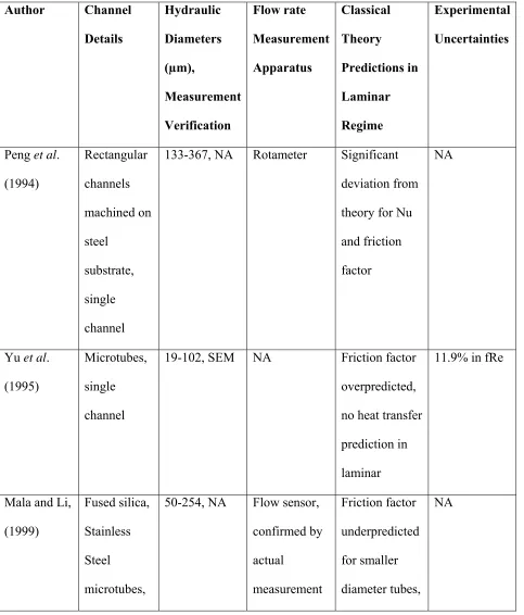
Table 2.1: Summary of investigation on single phase flows in microchannels

Author Channel Details Hydraulic Diameters (µm), Measurement Verification Flow rate Measurement Apparatus Classical Theory Predictions in Laminar Regime Experimental Uncertainties

Peng et al.

(1994) Rectangular channels machined on steel substrate, single channel

133-367, NA Rotameter Significant

deviation from

theory for Nu

and friction

factor

NA

Yu et al.

(1995)

Microtubes,

single

channel

19-102, SEM NA Friction factor

overpredicted,

no heat transfer

prediction in

laminar

11.9% in fRe

Mala and Li,

(1999)

Fused silica,

Stainless

Steel

microtubes,

50-254, NA Flow sensor,

single

channel

no heat transfer

study.

Hegab et al.

(2001) Milled Aluminium plates, multiple channels 112-210, digital dial calipers

Flowmeter Agreement for

friction factor,

no heat transfer

study

3-23% for

friction factor

Bucci et al.

(2003)

Microtube,

Single

channel

172-520, NA Friction factor

agreement

below Re

800-1000, heat transfer coefficient higher than thermally developing flow theory Solomon and Sobhan, (2005) Milling copper plates, multiple channels

280-3670, NA Rotameter fRe

underpredicted, Nu over predicted NA Steinke and Kandlikar, Etched Silicon

222, SEM Rotameter Agreement for

fRe and Nu

(2005) channels,

multiple

channels

Rands et al.,

(2006) Fused silicon microtubes, single channel

16-30, SEM Graduated

flask and stop

watch

Agreement

with theory for

fRe, no heat

transfer study

16-29 % for

fRe Hrnjak and Tu, (2007) Machined in PVC substrate, single channel 69-304, Stylus surface profilometer Rheotherm® mass flow meter Agreement for friction factor,

no heat transfer

study

±3.5% for f

Peng et al. (1994) began investigating into the microchannel performance in comparison

to the conventional theory. They found a discrepancy in the two. They experimentally

investigated heat transfer in rectangular microchannels with hydraulic diameters of 133-367µm.

Their experiments indicated early transition to turbulent regime and fully developed flow was

observed for Re 400-1500. Nusselt number in the laminar regime was found to be dependent on

Re0.62. Fluid properties were calculated at the fluid inlet temperature. The relationship between

friction factor and Nusselt number was observed to be significantly different for the laminar

flow. The authors stated that for microchannels the friction factor in the laminar regime was

that the experimental friction factor was higher than the classical prediction. The laminar to

turbulent transition was found to be a strong function of the hydraulic diameter.

Mala and Li (1999) investigated water flow through tubes of diameters ranging from 50

to 254μm. The flow characteristics for smaller tubes deviated significantly from the conventional

theory. Material dependence on the friction factor was observed and the values obtained

experimentally were higher than the predictions. At lower flow rate the results were in rough

agreement with the theory however, significant deviation was noted at higher Re flows. Two

possible explanations were discussed. One was that there was early rise to transition flow and

hence laminar flow equations cannot be used. The second reason which also explained the early

transition was the surface roughness which might be thought to play an important role. It was

however apparent that the early transition seemed to be the prominent reason for the discrepancy.

Harms et al., (1999) applied the developing flow theory for both single channel and

multiple channel systems to characterize flow and heat transfer in minichannels. The channels

were 1000µm deep and 251µm wide. They experimentally observed that the local Nusselt

number agreed well with the classical developing flow theory. However, for multiple channel

design, agreement was reasonably well at higher flow rates but deviated significantly from

theory at low flow rates. Authors reported this deviation to the flow bypass in the manifold. But

it was concluded that the classical theory does apply to plain microchannels as well

Hegab et al. (2001) found that the friction factors values were consistently lower than

values predicted by macroscale correlations in the transition and the turbulent regime. R-134a

was used as the test fluid for 112-210 μm hydraulic diameter rectangular channels. For the heat

transfer calculations at lower Reynolds numbers, the uncertainties reported were as high as 67%.

Hrnjak and Tu (2007) investigated fully developed liquid and vapor flow through

rectangular microchannels with hydraulic diameters of 69 to 304μm. For low surface roughness

the flaminar approached the conventional values for all the channels tested. No heat transfer studies

were performed.

Steinke and Kandlikar (2005) conducted an exhaustive survey of literature and

experimentally investigated friction factor and Nusselt number in silicon microchannels. They

used the simultaneously developing flow condition since the channel lengths were small, and

compared the data with the developing flow theory. It was reported that the developing flow

theory was in very good agreement with the data. It may be noted that the individual channel

dimensions were measured and were very close to each other.

It is observed from literature that there are contradictory findings, especially as related to

the applicability of the laminar flow theory for microchannels flows. However, there seems to be

a consensus building up in the recent years which agree that fluid flow in microchannels in the

laminar regime is not different from macroscale phenomenon in some of the carefully conducted

experiments with same size channels. Although the continuum assumption is widely accepted for

microchannels, the effect of individual channel size variations is believed to be a factor

responsible for these deviations in parallel microchannels. This work attempts to analyze the

effects of flow maldistribution on the single phase flow predictions in microchannels.

2.2 Enhanced Microchannels

Enhanced microchannels mentioned here on refer to the offset strip fin configuration.

This type of minichannel configuration has been widely researched for many decades for its very

high heat transfer surface area. For the design of such a heat exchanger it is very essential to be

cooling, not many papers have dealt with rectangular offset strip fins microchannels. Recently

Kosar and Peles (2006), Prasher et al (2007) have investigated offset pin fin geometry. Steinke

and Kandlikar (2006) and Colgan et al (2005) are the two publications with data on enhanced

microchannels. However, for mini channel offset strip fin geometry, various researchers have

collected data and many correlations have been developed. The scope of current work is

extended only towards adiabatic flow in microchannels.

Kays (1993) developed a very simple analytical model for predicting hydraulic

performance of enhanced channels. This earliest model was based on the forced convection on a

plate with an additional term which included the drag coefficient. Weiting (1977) obtained

correlations from curve fits to data from over 20 core geometries covering laminar and turbulent

ranges. Sparrow and Liu (1979) investigated numerically the heat transfer and pressure-drop

results for laminar airflow through arrays of inline or staggered plate segments. Joshi and Webb

(1987) presented analytical models to predict the heat transfer coefficient and the friction factor

of the offset strip fin heat exchanger surface geometry in the laminar and turbulent flow regimes.

They also studied the transport of energy and momentum in the boundary layers of the fins

because of the oscillating velocities developed from the wakes. Thus the wake distribution was

also studied by them to take into considerations the effect of fin length, fin thickness and the fin

spacing on the wake flow pattern. This was done to accurately determine the transition flow. The

models developed are very complicated. Manglik and Bergles (1995) gave an exhaustive

summary of the existing correlations for minichannels. They also developed a correlation with a

consistent definition of hydraulic diameter. The equations for friction factor were a continuous

Fig. 2.1: Manifold images from side facing the channel and channel chip, Colgan et

al (2005)

All this work has been carried out at the minichannel level, with the flow ranges

occurring in the practical application of around 200-4000 Reynolds number. Also almost all the

predictive models developed are based on multiple regression analysis. The application of these

correlations for microchannel data needs to be ascertained.

Colgan et al (2005) obtained data on enhanced microchannel for laminar flow regime

with the Reynolds number in the range of 20-300. They obtained cooling of over 300 W/cm2

with very little pressure drop. This was achieved by designing an intricate manifold structure

interconnected to each other rather than just an elongated opening which serves as the inlet.

Figure 2.1 shows the photograph of the manifold facing the chip. The result of the multiple inlet

and outlet inlet vias leads to a complex and short flow lengths which significantly enhance the

performance. As a result this data cannot be used as a comparison to test the minichannel

correlations due to heavy cross flows caused by the multiple inlets and outlets.

Bapat and Kandlikar (2006) investigated the minichannel correlations used to predict

offset strip fin heat exchanger performance. The correlations were compared with experimental

microchannel data on offset strip fins obtained by Colgan et al (2005). Two reasons were cited

correlations are based on series of experimental data collected on various geometries. The flow

ranges employed in gathering that data were in the practical limits of 200-4000 Reynolds number

range. For laminar flow which is normally used in microchannels, the range is around 20-200

Reynolds number. Thus the correlations should be tested with large data sets on various aspect

ratios. The second reason cited was that the experimental data used for comparison is not a good

reference. The microchannel coolers are very advanced with very short flow lengths and multiple

inlets and outlets which are responsible for a complex flow path. Thus the data may not be

represe

ed microchannels. Fluid flow in enhanced microchannels is

predicted using CFD in this work.

2.3

predicted using CFD. FLUENT, commercially available CFD software is used to predict the ntative of simple offset strip fin microchannels.

Enhanced microchannels with offset strip fin configuration provide an attractive

alternative for electronics cooling application. However no predictive model has been developed

to predict the fluid flow in enhanc

Objective

This work addresses two points evident in the literature review. For plain channels it is

seen that although there are few investigations which show that the classical equations can

predict the microchannel flow, there are some experiments which show that there is deviation

from the theoretical prediction. Flow maldistribution in parallel plain microchannels is believed

to be one of the reasons for this discrepancy. This premise is experimentally investigated by

analyzing frictional pressure losses in parallel microchannels. Also, for enhanced channels, it is

seen that there is no analytical model developed yet to predict the fluid flow performance. Also

the existing correlations based on minichannels are not applicable to the microchannel data. The

performance. Experiments are also carried out to validate the computer simulations. Following

are the objectives of the thesis

• To estimate flow maldistribution in parallel microchannels induced by channel size

variation

• Experimentally evaluate the effect of flow maldistribution on the friction factor

prediction using classical fluid flow equations

• Predict the fluid flow performance in enhanced microchannels using CFD analysis

• To experimentally validate the CFD results on adiabatic flows in enhanced

microchannels

• Test the validity of existing enhanced minichannel correlations to predict the

CHAPTER THREE

EXPERIMENTAL SETUP FOR PLAIN MICROCHANNELS

It is identified from the literature that there is discrepancy in the validity of the classical

equations for plain microchannels. Maldistribution is thought to be one of the reasons for this

deviation from theory. The typical test setup consists of a common inlet and outlet header

feeding parallel channels. Slight variation in the dimensions of the channel could lead to flow

maldistribution. This work investigates the effects of flow maldistribution on the friction factor

prediction for microchannels. This is experimentally investigated by machining six parallel

microchannels with different cross sectional areas to introduce flow maldistribution. This chapter

describes the design of the experimental setup for investigating the effects of flow

maldistribution on friction factor predictions in microchannels. The setup consists of a storage

tank, water pump, digital flow meters, a set of parallel microchannels and a receiver tank. The

following sections describe in the detail the flow circuit, instrumentation and data acquisition

circuit and the experimental procedure for the investigation for flow maldistribution on the

3.1 Flow Loop

Tin°C

Water Tank

Test Section

Δp

Water

Pump Digital Flowmeter Receiver

Fig. 3.1: Flow loop for investigation single phase flows in plain microchannels

A schematic of the experimental loop is shown in Fig. 3.1. Degassed water is stored in

the tank. The pump directs the water from the tank to the test section through a set of digital flow

meters. Two flow meters one with 0-100ml/min and other with 100-1000ml/min capacity are

used in parallel. This is an open loop and the heated water is led into a receiver where the flow

3.2 Test Section Design

Microchannels

Thermocouple Inserts

Cartridge Heater Housing

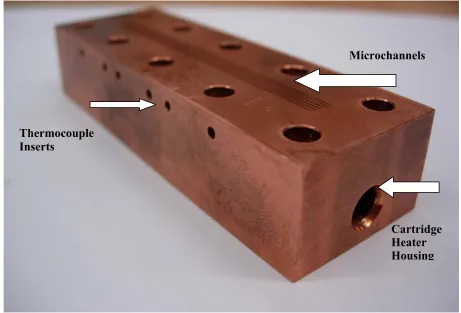
Fig. 3.2: Photograph of Copper Block Test Section with Parallel Microchannels

Figure 3.2 shows the actual photograph of the test section. It is a copper block with 6

parallel microchannels milled on the top surface. It has a hole below the microchannels which

houses a cartridge heater which is used to heat the surface of he channels. It has two layers of

thermocouples inserted on either sides of the copper block. The two layers are underneath the

copper surface at two different heights so that heat flux normal to the surface of the channel

Pressure Tap

Fig. 3.3: Photograph of cover plate with inlet and outlet manifolds

Figure 3.3 shows the header made of polycarbonate with the inlet and outlet manifolds.

The water flow is marked on the diagram. It enters through the inlet manifold into the

microchannels and then exits through the outlet header. The passage which connects the two

manifolds with the inlet and outlet connections also has a provision for inserting thermocouples.

E- type thermocouples are used. This ensures accurate inlet and outlet manifold temperatures.

Also taps are provided on the inlet and outlet passage for measuring the pressure drop across the

channel.

Pressure Tap Hot Water Out Cold Water In Thermocouple

Acrylic Header Plate

Copper Test Block

Phenolic Base

Fig. 3.4: Assembly of the cover plate, test section and the insulating base

Fig. 3.4 shows the three layer assembly of the test section. The bottom of copper block is

attached to a phenolic base. This acts as an insulating block. This assembly is mounted on a

3.3 Channel Dimensions

Table 3.1 Individual channel dimensional variability

CHANNEL 1 2 3 4 5 6

Mean Height µm

209.3 207.3 194.0 190.1 208.4 210.1

Mean Width

μm

268.5 264.6 265.8 262.3 236.9 266.4

Cross Section Area Acx102

μm2

560 546 514 498 492 559

The current test section has six parallel long channels. The individual channel dimensions

are measured using a surface profilometer at 11 different locations along the flow length. Table

3.1 gives the height and width of each channel along with the cross sectional area of each

channel. It is seen from the cross sectional area that channel one and five have the maximum and

minimum cross sectional area respectively. Thus actual flow in these channels is going to vary

the most for same pressure drop across these channels. Later when comparison will be made to

check the effects of flow maldistribution, these two channels are considered for comparison

purpose.

Fin Top Surface

3.4 Instrumentation and Data Acquisition

Pressure is measured using a differential pressure transducer. The pressure transducer is

a PX-26 series from Omega. The transducer is a silicon diaphragm that uses a wheat-stone

output is from 0 to 100 mV. The pressure transducer range is selected to give the highest level of

accuracy, with a range of 0 to 6.8 atm. The pressure transducers are calibrated using known

pressures and the measured response of the transducer. A pressure calibrator from Omega is

used to apply a known value of pressure. The range of the pressure calibrator is -100 to 200 kPa.

The high side pressure port on the differential pressure transducer is exposed to the known

values of pressure. Over twenty points are taken within the range of the specific pressure

transducer. A linear curve fit is assumed and used to generate the calibration equation. If the

range of the pressure transducer is 690 kPa, the transducer is calibrated up to 200 kPa and linear

behavior is assumed thorough the remainder of the range.

A gear pump manufactured by Micropump, Inc., model: GA-V23.J9FS.G, is used to

pump the working fluid. The maximum allowable pressure setting is 172 kPa, and it can deliver

a flow rate ranging from 42 mL/min to 350 mL/min. The pump has a pulsation of 1.5%. Water

is pumped through this pump. LabVIEW is also used to control the pump output by sending 0-5

DC voltage.

Two digital flowmeters (FLR 1007 and FLR 1010 from Omega) are used to accurately

measure the flow rate. The FLR 1007 model measures flow rate from 10-100 ml/min while the

FLR 1010 is for 100-1000 ml/min. The excitation voltage is 12.8 volts DC. The flow rate is

measured by a miniature turbine wheel housed inside the flow meter. The wheel rotates with a

speed proportional to volumetric flow rate of the fluid. The output signal of the flowmeters is

compared with the set point for the flow rate and the pump is controlled according to the

3.5 Experimental Uncertainties:

The uncertainty is determined by the method of evaluating the bias and precision errors.

The following equation is used to calculate the uncertainty in the experimental results which is

based on Kline and McClintock (1953).

2 2 2 2 2 1

1 ⎟⎟⎠

⎞ ⎜⎜ ⎝ ⎛ ∂ ∂ + ⎟⎟ ⎠ ⎞ ⎜⎜ ⎝ ⎛ ∂ ∂ + ⎟⎟ ⎠ ⎞ ⎜⎜ ⎝ ⎛ ∂ ∂ = _n n U v R U v R U v R U _K (3.1)

where U, R, and v are uncertainty interval, result, and variable, respectively.

The pressure transducer has an uncertainty of ±0.69 kPa. The temperature reading has an

uncertainty of ±0.1°C. The power supply used to provide input power within ±0.05 V and current

within ±0.005 amps uncertainty. The flow meter uncertainty in the volumetric flow measurement

is ±0.0588 cc/min. The power measurement has an accuracy of ±0.5 Watts. The temperature

difference measurements have an uncertainty of ±0.2°C. The resulting uncertainties are

calculated for the pressure drop is 7.19%, and friction factor is 4.80%, at a median flow case.

The major source of error is the temperature reading. This uncertainty is based on Steinke and

Kandlikar [14] as the same instrumentation setup is used.

3.6 Experimental Procedure

Water is first degassed to ensure homogeneity of the medium. This is done by boiling the

water in the storage tank and increasing the pressure to around 15 psi and then venting the

pressure. This is repeated twice. Water at atmospheric condition and over 90 °C releases all the

dissolved gasses. This degassed water is then allowed to cool down to room temperature. The

current study focuses on the classical equations based on the laminar flow regime. Thus the

A pump is used to direct the flow from the storage tank to the test section through flow

meters. The flow rate is recorded in LabVIEW and flow rate is compared with the set point. This

feedback is used to control the pump in order to push the exact quantity of water through the

circuit. The pressure drop across the inlet and outlet header is measured by the differential

pressure gage. Inlet temperature of water is also measured for determining the viscosity of fluid.

Readings are recorded only after the flow has been stabilized.

Pressure drop readings and the corresponding flow rates are recorded and are used to

calculate the apparent friction factor in each channel. Apparent friction factor includes the

pressure drops due to both developing and fully developed flow. The experimental value is

compared with the theoretical value to compare the effects of maldistribution on flow prediction

CHAPTER FOUR

EXPERIMENTAL SETUP FOR ENHANCED MICROCHANNELS

There has been very few data on enhanced microchannels. Enhanced Microchannels are

capable of dissipating very large quantities of heat because of periodic interruption of boundary

layer. However very high pressure drops are also encountered in this flow. Because of the

complexity of the flow caused by the flow over the fins, there has been no analytical solution to

predict the performance. In such a situation, predictive models are basically based on numerical

models or correlations which need lot of experimental data. For minichannels, of similar

configuration, there has been extensive research and many correlations have been developed

based on the existing data. However, there has been no predictive model yet developed for

enhanced microchannels. In this study, the pressure drop data is numerically modeled using

CFD. Also, experiments are also carried out to validate the numerical results and existing

minichannel correlations are tested on this data. Simple pressure drop experiments are carried out

on one offset strip fin silicon microchannel for the above purpose.

Experiments on an enhanced silicon microchannel are carried out for flow range of

20-200 Reynolds number in order to validate the numerical scheme. The following sections will

describe the flow loop and experimental procedure.

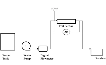
4.1 Flow Loop

A simple flow circuit is used which includes a pump, different pressure sensor and the offset

ΔP

Data Acquisition Peristaltic

Pump

Temperature Probe

Water Receiver

Enhanced Microchannel

Test Section

Fig. 4.1 Schematic of the Flow Loop for Enhanced Microchannels

Flow rates up to 80ml/min for water can be circulated through the enhanced

microchannels using the peristaltic pump. This roughly translates to around 250 Reynolds

number. Pressure drop is measured using a pressure deferential transducer. Temperature of the

water is also recorded before it enters the channel. This value of temperature is used to calculate

4.2 Test Section Details

The actual silicon microchannel is shown in fig. 4.2. The overall dimensions of the chip

are 10X10 mm. There are 80 channels with channel width of 50 µm and height of 200 µm across

the flow length while along the flow length; there are 40 rows of fins with fin length of 250 μm.

Fins have smooth entry and exit passages. The silicon chip is housed inside a cavity which is

then covered with an acrylic plate. Figure 4.3 shows the cover plate with the chip underneath it.

Chip Header

Parallel

Microchannels

Fig. 4.3: Text Fixture Housing the Silicon Microchannel

The pump outlet connection is made with the inlet connection for the test fixture. The

path takes a 90° bend to reach the header on the chip. Similar path is taken by the fluid while

exiting the channels. Pressure drop is measured across the inlet and outlet feed lines. This

pressure drop does include entry and exit losses associated with the area changes. These losses

are deducted from the measured pressure drop.

For the enhanced channels only adiabatic flow is investigated just like plain

microchannels. Experiments are carried out for flow in the laminar flow regime and the pressure

drop across the channels is calculated. This data is then compared with the minichannel

microchannels, numerical modeling is carried out in order to predict the microchannel pressure

drop data. The next chapter deals with the setup for the simulation of microchannel flows in

offset strip fin configurations.

4.3 Test Procedure:

Very high pressures are observed in enhanced channels. Experiments are carried out in

the laminar flow regime and at very flow Reynolds number range of 20-200. This range is

selected as because of the large frictional losses encountered in microchannels, laminar flow

regime is employed in practice. The pressure drop across the channels is measured with a

differential pressure gage while the volumetric flow rate is given by the peristaltic pump. Steady

CHAPTER FIVE

NUMERICAL SETUP FOR ENHANCED CHANNELS

Enhanced microchannels with offset strip fin configuration have not been extensively

researched in the literature. There have been no predictive models developed yet for the same.

Since performance of these microchannels is not evaluated, a numerical modeling is carried out

to verify whether the enhanced microchannel flow can be modeled using the classical flow

equations. The pressure drop is this numerically predicted using numerical modeling based on

finite volume method. Commercially available Computational Fluid Dynamics Solver FLUENT

is used for the computer simulations. It involves first recreating the flow geometry with the

region of interest, assigning correct boundary conditions, meshing of the geometry, and then

solving the Navier-Stokes Equation along with the continuity equation for prediction the pressure

drop in the flow. This chapter discusses in detail the problem setup for the numerical modeling

for pressure drop in enhanced microchannel. Heat transfer is not modeled in this work.

5.1 Flow Geometry:

The geometry is created and meshed using GAMBIT. The enhanced chip as described in

the above section contains 80 of fins in the transverse direction with fin lengths of 250 μm. The

total flow length is 10000μm which implies around 40 fins along the flow length. This type of

repeated geometry makes the flow also repeatable after initial few rows of fins. Since the number

of fins along the flow length is very large, it is a safe assumption to model the flow after a steady

flow has been established. This is called as the periodic flow condition which is different than

create identical flow path. Figure 5.1 shows a highly magnified image of the fin structure for the

chip under consideration.

Fig 5.1: 1000X magnified image of offset strip fins from KEYENCE microscope

The numbers marked in the snapshot have the following values; 1-50µm, 2-50µm,

4-100µm. It is clear from the figure that the fins do not have flat front faces. There is a smooth

entry and exit for the fluid into the channel. This geometry is very difficult to create in

GAMBIT. An approximation is used to create this geometry. Marked on the above figure you

see the dimensions which are used to make the geometry. Figure 5.2 shows the schematic of the

Fig. 5.2 Schematic of Unit Cell and Computational Domain

Computational

Domain/ Unit Cell

Flow

Direction

Fig. 5.3 Image of Unit Cell created in GAMBIT

Figure5.3 shows the actual 3D model which is created in GAMBIT which is the graphical

representation of the schematic of the computational domain. The symmetry and periodic nature

of the flow which is inherent in the flow is the reason for modeling on part of geometry in

FLUENT. The boundary conditions which are applied to this geometry are discussed in detail in

the following section.

Fin Walls

Fin Walls Fin Walls

Inlet

Outlet Symmetry

Surface

5.2 Zone Specifications

The physical and the operating characteristics of the computational model at its

boundaries are given by the zone type specifications. There are basically two types; Boundary

Type and the Continuum Type.

The Continuum Type is set to fluid for the current setup. This enables to characterize the

unit cell within the domain as a fluid. The momentum and continuity equations are applied to the

nodes or the cells that exist within the volume. Since the unit cell is a 3D representation of the

enhanced channels, the boundary conditions are specified for the faces of the model. Each face

or boundary of the model needs to given a boundary condition. Following are the conditions

specified.

Wall Boundary Condition: The no slip boundary condition is given by assigning the faces

as wall and giving the zero velocity. The top, bottom and fins are given the no slip condition

Symmetry: The unit cell is the representation of the complete enhanced channel. The unit

cell can be replicated along the symmetry lines. The symmetry faces are marked on the fig. 5.3.

By specifying symmetry boundary condition, the flow and pressure gradients are identically zero

along these faces. Because of this the physical conditions in the regions immediately adjacent to

either side of the edge are identical to each other.

Periodic Boundary Condition: The inlet and the exit faces of the domain are marked as

periodic. The mesh on these faces also need to be linked. When these faces are hard linked,

GAMBIT associates the faces with each other. And any operation applied to one face is linked

with the other face. In other words, the flow characteristics are at the exit face are replicated at

the inlet wall. This leads to a “fully developed” flow condition. The term fully developed does

not assume the conventional meaning. For the present case, the term fully developed refers to the

same flow pattern is obtained in the preceding and following unit cells. This is one of the

assumptions which is used while modeling the flow in enhanced channels. The boundary

conditions for the unit cell are clearly marked on the faces as shown in fig. 13.

5.3 Mesh Generation

The enhanced channel is approximated using all rectangular faces. Since the geometry is

computational very straightforward, Quad Elements are used for meshing. This specifies that the

mesh includes all quadrilateral mesh elements. For each mesh element have a range of meshing

schemes that can be used. A Quad-Map Meshing scheme is used which creates a regular,

structured grid of mesh elements. Quad-Map meshing scheme is applicable primarily to faces

that are bounded by four or more edges and also the face should be logically rectangle [FLUENT

docs ref]. As the geometry satisfies both these conditions a Quad Map Meshing Scheme is used.

163200 mesh volumes are created for the geometry. Figure 5.4 shows a top view of the meshed

Fig. 5.4: Meshed Unit Cell of Enhanced Microchannel

5.4 Mesh Quality

It is important before the simulations are run that the mesh quality be checked. If the

choice of meshing scheme is not correct, the results of the numerical modeling may not make

any sense. EquiAngle Skew and MidAngle Skew are used to test the mesh quality. EquiAngle

Skew is a normalized measure of skewness. QEAS=0 suggest a equilateral element while QEAS=1

represents a completely degenerate or poorly shaped element. The MidAngle Skew or QMAS

applies only to quadrilateral and hexahedral elements. By definition of QMAS its value also lies in

documentation. It is assumed that in general high quality meshes contain elements that possess

average QEAS values of 0.1 for 2D element and 0.4 for 3D element.

For the current Quad-Map Meshing Scheme, 100% of total mesh elements have QEAS

value between 0 and 0.3 with worst element having a value of 0.295 while 90% of the total mesh

elements have QMAS value fall in the range of 0 and 0.3 with the worst element having value of

0.41. Thus overall for the type of geometry under consideration, the mesh quality is very good.

5.5 Mesh Size Dependence

Trial runs are performed on the meshed geometry to check the mesh size sensitivity.

Mass flow rate of 2.4732e-6 kg/s is given to the unit cell for 3 different mesh sizes. The pressure

gradient computed by FLUENT to maintain the specified flow rate is compared. Table 5.1 gives

the mesh size, the value of pressure gradient for above given flow rate and the percent change in

the pressure gradient.

Table 5.1: Mesh Size Sensitivity

Mesh Size

µm

Pressure Gradient

Pa/m

% Change in Pressure

Gradient

2 2206444 0.3

2.5 2213288 0.1

3 2217718 -

It is seen from the Table 5.1, that by reducing the mesh size from 3 µm to 2.5 µm, there is

only 0.1 % change in the value of the pressure gradient, while changing the mesh size further

down to 2 µm, there is a change of 0.3 % in the result. Thus mesh size of 2.5 µm is selected as

the final mesh size. For 2 µm mesh size, the computational time increased a lot and since there is

negligible change in the result, mesh size of 2.5 µm was selected to save computational time.

Any further reduction in mesh size was not possible because of the processor limitations. For

mesh size of 2.5 µm a total of 163200 mesh volumes are generated.

This meshed mathematical model is simulated in FLUENT. The objective of this

simulation is to confirm if flow in enhanced microchannels can be predicted. Experiments in the

Reynolds number range of 20-200 are performed as described in chapter four. Hence for

numerical modeling, the same flow conditions are simulated which were used for the

experiments.

In Chapters Three, Four and Five, the setup for experimental and numerical analysis for

both plain and enhanced microchannels has been explained. The development of maldistribution

CHAPTER SIX

MALDISTRIBUTION ANALYSIS FOR PLAIN MICROCHANNELS

In the literature it is seen that there are contradictions on the applicability of conventional

fluid flow equations on the microchannel data. It is thought that flow maldistribution in multiple

channels could lead to this discrepancy in the literature. In this chapter, the maldistribution

analysis is explained in detail. This includes estimating the flow in each channel and then

estimating the friction characteristics and comparing it with theory. The following section

describes the logic behind the estimation of the maldistribution and the data comparison with the

theory.

For comparing the predictions based on maldistribution analysis with the uniform flow

assumption, the uniform flow calculations are similar except for non uniform analysis, individual

channel dimensions are considered while for uniform flow calculations each channel is assumed

to have the same dimension, which ensures that there is no flow maldistribution. The calculations

described below are for one with maldistribution. Same procedure is followed for uniform flow

analysis.

6.1 Estimating Flow Maldistribution

Figure 6.1 illustrates the test section designed to investigate the effects of flow

maldistribution on the prediction of friction factor using the classical equations. As described in

the Chapter Four, the copper block has 6 parallel channels machined on the surface and water is

shown in the schematic. Since for all parallel channels have the same pressure drop across its

end, the flow is uniformly distributed only if all the channels have the same dimension. However

as shown in the fig. 6.1 six channels of varying dimensions are shown. This results in flow

maldistribution in the channels.

m

, A

m

, A

m

, A

m

, A

m

, A

m

, A

T

Inlet

Header

Δ

P

Outlet

Header

Flow

Fig 6.1: Schematic of multiple microchannels with the inlet and outlet manifold

Mass flow rate can be expressed in terms of pressure drop Δp, apparent friction factor fapp

and Reynolds number Re by the following eq. (6.1).

(6.1) 2 . h c D A p

m Δ ρ

Re) (

2 f_app μ L

=

&

2

hi ci

i A D

m α

hi

D Aci

total

i m

m

where Ac and Dh are the channel cross sectional area and hydraulic diameter respectively,

fapp represents the apparent friction factor which includes the pressure drops due to developing

flow as well as fully developed flow.

For a channel with fixed cross section, the variables involved which would determine the

mass flow rate are fapp.Re and Δp. The channel length is around 55mm and for the flow rates

under purview of this study, the developing flow length is not significant and for fully developed

flows, the product fapp. Re is constant. The flow rate is hence dependent on the pressure drop and

the channel dimensions. From the above equation, mass flow rate in each channel for the

measured pressure drop can be found to be proportional to the product of cross sectional area and

the square of hydraulic diameter as shown in eqn. (6.2)

(6.2)

Where and are the hydraulic diameter and cross sectional area of the ith channel

and mi is the mass flow rate in that channel

The total flow rate is measured accurately using two digital flow meters. If mi is the flow

through channel i, then

∑

total hi ci hi ci i m D A D A

m ₂ .

2

∑

= (6.4)

This flow rate is considered henceforth while predicting the friction factor for the

individual channels.

6.2 Friction Factor Prediction

Once the mass flow in each channel is estimated, friction factor is found for each channel

and it is compared with the theory. Using the individual channel flow rate and the measured

pressure drop is used to calculate the experimental friction factor is each channel using the

following eqn. (6.5)

L m

D A p

fapp expt ci hi

. . . 2 . . . Re 2 & μ ρ Δ

= (6.5)

For theoretical value fapp,Re, table developed by Phillips (1987) for flow in rectangular

microchannels is used. It takes into account the pressure drop due to developing flow as well as

fully developed flow. However, in the present case, because the flow is nearly fully developed,

the value of fapp,Re tends to be same as fully developed flow for rectangular channel of that

aspect ratio. The expression for fappRe is given by Eq. (6.6). and the values of the constants a-f

are obtained from Kandlikar et al.(2005).

5 . 0

Re= a+cx+ +ex+

where the non-dimensional hydrodynamic entry length is represented by x+ given by the following equation: h D L x . Re =

+ _(6.7)

The above calculated value represents the theoretical friction factor in the channel for the

measured pressure drop and for the estimated flow rate in that channel. This theoretical friction

factor, eqn. (6.6) is compared with experimental friction factor given by eqn. (6.5) for all 6

channels. There are thus 6 different plots. However for the uniform flow analysis only one plot is

employed since all the six channels are of same dimension, same flow rate is used in each

channel and hence same theoretical and experimental flow rate for each channel. The plots are

presented in Chapter Eight.

Throughout the above mentioned calculations, the pressure drop was measured across the

inlet and outlet manifold. It includes the losses in the 90° bends and the expansion and

contraction losses. Equation (6.8) is used to calculate the pressure losses; K90, Kc and Ke

represent the coefficients for losses in the 90° bends, contraction and expansion losses. The

values for these coefficients are based on Phillips (1987).

ρ 2 2 90 2 2 2 . c e c p c l A m K K K A A p & ⎥ ⎥ ⎦ ⎤ ⎢ ⎢ ⎣ ⎡ + + ⎟ ⎟ ⎠ ⎞ ⎜ ⎜ ⎝ ⎛ =

The pressure drop Δp is referenced in this paper henceforth after deducting the pressure

losses from the actual measured pressure drop and represents the net pressure drop in the

microchannels. The apparent friction factor fapp is the non dimensional form representating the

same pressure drop.

The analysis presented here is applicable only to plain channels. For enhanced channels,

there is no analytical solution to predict the performance. Existing minichannel correlations are

tested with the new experimental data and the numerical modeling is validated by the data. The

next chapter details the minichannel correlations which are used to predict the enhanced

CHAPTER SEVEN

ENHANCED MICROCHANNELS – FRICTION FACTOR ANALYSIS

Minichannel offset strip fin heat exchangers have been used for a long time. As the name

suggests, these are called enhanced channels because of the enhancement in the heat transfer

achieved by periodically interrupting the fluid flow length. However, as a result of fins

interrupting the flow, wakes are formed and fluid mixing occurs. This makes it very difficult to

analytically predict the performance. All the predictive models developed so far for minichannels

with offset strip configuration have been based on either numerical modeling or correlations

which are based on experimental data collected on different aspect ratio channels. For

microchannels however neither numerical study has been carried out nor have any correlations

been developed. This work aims to evaluate the flow in enhanced microchannels by numerically

modeling the flow as well by generating experimental data and testing the validity of

minichannel correlations for this data. There are few correlations which have been widely used

for predicting performance in the minichannels. This chapter presents those correlations which

would be used to analyze the microchannel data.

7.1 Enhanced Microchannel Data Reduction

7.1.1 Experimental Friction Factor

Experiments were carried out an enhanced silicon microchannel for low Reynolds

number flow as described in Chapter Four. Table 7.1 gives the values of flow rates and the