Decomposition of nuclear magnetic resonance spin-spin coupling constants into active and passive orbital contributions

Decomposition of nuclear magnetic resonance spin–spin coupling

constants into active and passive orbital contributions

Ju¨rgen Gra¨fenstein, Tell Tuttle, and Dieter Cremera)

Department of Theoretical Chemistry, Go¨teborg University Reutersgatan 2, S-41320 Go¨teborg, Sweden 共Received 6 January 2004; accepted 2 March 2004兲

The theory of the J–OC–PSP共decomposition of J into orbital contributions using orbital currents and partial spin polarization兲method is derived to distinguish between the role of active, passive, and frozen orbitals on the nuclear magnetic resonance 共NMR兲 spin–spin coupling mechanism. Application of J–OC–PSP to the NMR spin–spin coupling constants of ethylene, which are calculated using coupled perturbed density functional theory in connection with the B3LYP hybrid functional and a 关7s,6p,2d/4s,2p兴 basis set, reveal that the well-known ␲ mechanism for Fermi contact共FC兲spin coupling is based on passive␲orbital contributions. The␲orbitals contribute to the spin polarization of the␴orbitals at the coupling nuclei by mediating spin information between

␴orbitals共spin-transport mechanism兲or by increasing the spin information of a␴orbital by an echo effect. The calculated FC共␲兲value of the SSCC1J共CC) of ethylene is 4.5 Hz and by this clearly smaller than previously assumed. © 2004 American Institute of Physics.

关DOI: 10.1063/1.1711598兴

I. INTRODUCTION

Nuclear magnetic resonance 共NMR兲 parameters such as chemical shieldings or spin–spin coupling constants

共SSCCs兲 provide important information about geometry, conformation, and other properties of a molecule.1– 8In gen-eral, magnetic parameters represent hypersensitive antennae that indicate features of the electronic structure which are difficult to detect by other means 共e.g., degree of electron delocalization in weakly aromatic or antiaromatic molecules; anisotropy of the electron distribution, density close to the nucleus, polarizability of the electrons, detection of electron currents, etc.兲. The use of the magnetic properties of a mol-ecule as suitable descriptors for electronic structure features requires of course that the dependence of a magnetic param-eter on other molecular properties is known and can be de-scribed with simple mathematical relationships. Convincing examples in this regard are the Karplus relationship共 depen-dence of the NMR spin–spin coupling constant J on the conformation of a molecule兲,9 the dependence of J on the s-character of a bond,10–13 charge-chemical shift relationships,14,15etc. Although many of the frequently used relationships are made plausible on an ad hoc basis, a basic understanding in terms of spin density distributions, electron excitations, electron currents, and intramolecular magnetic fields is missing.

The present work is part of a larger project aimed at developing the theory for calculating SS–CCs with the help of DFT,16 using SSCCs as conformational descriptors,17–19 and analyzing the mechanism of NMR spin–spin coupling in dependence of the electronic structure of a molecule and its bonding characteristics.20–28 Indirect spin–spin coupling is transmitted by four different mechanisms from a nucleus B,

which by its magnetic spin moment perturbs the surrounding electron density 共perturbing nucleus兲, to the nucleus A, the magnetic moment of which receives the perturbation of the electron density and responds to it 共responding nucleus兲:29

共1兲The Fermi contact共FC兲mechanism caused by the inter-nal magnetic field of nucleus B, which causes spin polariza-tion of the density at the contact surface of this nucleus. Spin polarization travels like a wave through the electron system and interacts with the spin moment of nucleus A. 共2兲 The spin dipole共SD兲mechanism, which arises from the spin po-larization caused by the external magnetic field of nucleus B.

共3兲The spin–orbit共SO兲mechanisms are associated with or-bital currents 共equivalent to electron currents兲 generated by the spin moment of nucleus B; the electron currents are ac-companied by a magnetic field, which is experienced by nucleus A. In the diamagnetic SO 共DSO兲case, there are cir-cular currents corresponding to a Larmor precession for each electron, which depend on the form of the orbital and the associated orbital density in the molecular ground state. 共4兲 In the paramagnetic SO共PSO兲case, the orbital currents de-pend on the existence of appropriate excited states that can be reached from the ground state of the system by suitable excitations with not too large excitation energies.

Although the spin–spin coupling mechanism is indepen-dent of the direction in which the coupling information is moved from one nucleus to the other 共B→A as used in this work or A→B兲, the coupling mechanism can be more easily explained if one nucleus is always considered as the perturb-ing and a second nucleus is considered as the respondperturb-ing nucleus thus leading to the SSCCnJ共AB) where n gives the number of bonds in the shortest coupling path. If one con-siders organic molecules, for which most of the early NMR measurements were carried out,2– 8the four spin–spin cou-pling transmission mechanism associated with the Ramsey a兲_{Author to whom correspondence should be addressed. Electronic mail:}

[email protected]

9952

terms can be characterized according to the electrons共 orbit-als兲involved in them.

The DSO mechanism involves all electrons. Although the individual components of the DSO term can be signifi-cant, they cancel each other largely out so that the DSO term in general is small and can be neglected. The sign and mag-nitude of the FC term depend on the properties of the s␴spin density distribution at the responding nucleus20 whereas the sign and magnitude of the SD term are determined by the p␴ and p␲-spin density distribution.22 The p␴ and p␲ orbitals also determine the sign and magnitude of the PSO term al-though the transmission mechanism is now based on orbital currents generated by the perturbing nucleus and detected by the responding nucleus.21,24

At a first glance, it seems that␲ electrons do not play any role for the FC spin coupling mechanism because these electrons have no spin density at the contact surface of a nucleus. Nevertheless, one knows that long range spin–spin coupling leading to sizable values of SSCCs 4J or 5J in

conjugated hydrocarbons is dominated by a ␲

mechanism.4,5,30–36Similar to the case of the ESR hyperfine coupling constants a(•C–H) or a(•C–C–H), which result from spin polarization of the␴system by an unpaired elec-tron in a C p␲ orbital,37 the NMR spin–spin coupling mechanism is transferred via the␲electrons to the s␴ spin density at the responding nucleus.4,5,30–36

Clearly the ␲ electrons participate in the FC coupling mechanism in a passive rather than active way, i.e., they are not directly affected by the internal magnetic field of the perturbing nucleus. This passive contribution has been shown to be always present in any␲system where differing reports about the magnitude of the␲ mechanism have been made.4,5,30–36 In this work, we will focus on the ␲ mecha-nism, determine the magnitude of the FC共␲兲part of the total FC term, and describe the ␲ mechanism in detail. In this connection we will investigate the following two questions:

共1兲 In which ways can the␲ orbitals contribute to the transmission of spin information between the coupling nuclei considering the fact that they can neither be polarized di-rectly by the perturbing nucleus nor transfer spin information to the responding nucleus? How can the contribution of the

␲ orbitals to the FC coupling mechanism be quantified and how can it be visualized? For the purpose of answering these questions we will develop needed theory and computer soft-ware that can be routinely applied for any passively acting orbital.

共2兲 How important is the␲mechanism for SSCC across a double bond? Semiempirical calculations with a minimal basis set33–36suggest that a significant portion of the FC part of1J共CC) in unsaturated hydrocarbons共up to 20% or 15 Hz兲 is related to contributions from the␲electrons. To what ex-tent can these findings be confirmed by DFT calculations with an extended basis set? For the purpose of answering these questions, we will develop in Sec. II the theory of passive spin–spin coupling interactions and incorporate it into the recently described J–OC–PSP共decomposition of J into orbital contributions using orbital currents and partial spin polarization兲 method.20 We will define active, passive, and frozen orbitals for the spin–spin coupling mechanism.

Furthermore, we will use the FC spin density distribution to visualize the ␲mechanism. All calculations will employ the coupled perturbed density functional 共CP–DFT兲 method16 because we have shown that this is most suitable and reliable for larger hydrocarbons.15–19 In Sec. III, the ␲ mechanism will be discussed for the simple case of the SSCCs of ethyl-ene. We will show the different modes of interaction between

␴ and␲ electrons and work out the general features for FC coupling via ␲ orbitals. These features will be verified by determining those calculational tools important for the de-scription of the␲mechanism, which will provide a basis to compare previous calculations of the FC共␲兲 part with the present one. We will show that the ␲ mechanism, although rather important for long-range coupling, does not play such an important role for short-range coupling as was previously assumed.

II. THEORY OF THE SPIN–SPIN COUPLING MECHANISM

CP–DFT used in this work to calculate NMR SSCC was described elsewhere.16 We will use CP–DFT in connection with the J–OC–PSP method20 to determine the orbital con-tributions to the four Ramsey terms. For this purpose, we briefly review the CP–DFT equations, which for canonical orbitals read

兩␸k共 B兲

_典

_⫽

兺

a

具

␸a共

0兲_兩F共B兲_兩␸ k 共0兲

_典

⑀k⫺⑀a 兩␸a

共0兲

_典

_{. 共1兲}

Here, F(B)is the first-order KS operator for a perturbation X

共X⫽PSO, FC, or SD兲at nucleus B, and兩␸_k(B)

典

are the first-order orbitals corresponding to F(B). For brevity, we omit in this section the index X specifying the kind of perturbation. Furthermore, we will not distinguish explicitly between space and spin orbitals.

The analysis of SSCCs is done not in canonical MOs but in localized MOs 共LMOs兲, which reflect the intuitive under-standing of the electron system in the molecule共core orbit-als, bonds, lone pairs兲. The LMOs␺_kare connected with the canonical MOs by an orthogonal transformation matrix u,

兩␺k共 0兲

_典

_⫽

兺

l

u_kl兩␸_l共0兲

典

, 共2a兲

兩␺k共 B兲

_典

_⫽

兺

l

ukl兩␸l共

B兲

_典

_{. 共2b兲}

Equations共2a兲and共2b兲are valid for not only LMOs but for any representation of the MOs. If LMOs are used the orbital energies⑀k must be replaced by the zeroth-order KS matrix

F_kl(0), which leads to a coupling between the CP–DFT equa-tions,

兩␺k共 B兲

_典

_⫽

兺

a

具

␺a共

0兲_兩F共B兲_兩␺ k 共0兲

_典

_⫺

兺

l,l_⫽k

F_kl共0兲

具

␺_a共0兲兩␺_l共B兲

典

F_kk共0兲⫺⑀_a 兩␺a

contri-bution F˜(B)_{that covers the feedback of the first-order orbitals}

to the KS operator. The latter can in turn be decomposed into contributions from the individual orbitals:

F共B兲⫽h共B兲⫹F˜共B兲, 共4a兲

F ˜共B兲_⫽

兺

l

F ˜

l

共B兲_{, 共4b兲}

F ˜

l

共B兲_⫽

冕

_d3_r ␦F ␦␺l共

0兲␺l共

B兲_{共r兲. 共4c兲}

With this decomposition, Eq.共3兲takes the form

C_ak共B兲⫽ 1 Fkk共

0兲_⫺⑀ a

冋

h_ak共B兲⫹共˜F_k共B兲兲ak⫹

兺

l,l⫽k共共

F ˜

l 共B兲_兲

ak

⫺F共_kl0兲C共_alB兲兲

册

. 共5兲

For brevity, we have introduced the notation C_ak(B) ⫽

具

␺a

(0)_兩␺ k (B)

_典

and denote matrix elements of the form

具

␺p (0)_兩

Oˆ兩␺_q(0)

典

⫽Opq.

The matrix elements F˜ak (B)

can be determined by compar-ing two equivalent expressions for the coefficient matrix C_ak(B). In general, it can be written as

C_ak共B兲⫽⫺

兺

k⬘a⬘

共H兲_ak,a⫺1 _⬘k⬘h共_aB_⬘k兲_⬘. 共6兲

Here, H is the full orbital Hessian, i.e., the matrix

H_ak,a⬘k⬘⫽ ⳵

2_E

⳵Cak⳵Ca⬘k⬘

冏

_C⫽0

共7兲

containing the second derivatives of the ground-state energy with respect to simultaneous orbital rotations k→a, k

⬘

→a

⬘

. The explicit form of H can be found elsewhere.38 Equation共5兲can be rearranged into

Cak共 B兲_⫽⫺

兺

k⬘a⬘

关H共0兲兴_ak,a⫺1 _⬘k⬘F_a共B_⬘k兲_⬘, 共8兲

where

H_ak,a共0兲 _⬘k⬘⫽

兺

k⬙a⬙

ukk⬙uk⬘k⬙uaa⬙ua⬘a⬙共⑀a⬙⫺⑀k⬙兲 共9兲

is the zeroth-order Hessian, which results from the full Hes-sian H by omitting all terms related to two-electron interac-tions. Note that uaa⬘⫽␦aa⬘and H(0)will be diagonal in aa

⬘

if the virtual orbitals are kept canonical. In this special case, the zeroth-order Hessian takes the form

H_ak,a共0兲 _⬘k⬘⫽␦aa⬘共⑀a⫺Fkk⬘

共0兲_{兲. 共10兲}

Comparing Eqs.共6兲and共8兲gives

F_ak共B兲⫽

兺

k⬘a⬘k

兺

⬙a⬙

H_ak,a共0兲 _⬙k⬙共H兲_a⫺_⬙1_{k⬙,a⬘k⬘}h_a共B_⬘k兲_⬘, 共11a兲

F ˜

ak

共B兲_⫽⫺

兺

k⬘a⬘ k

兺

⬙a⬙

H˜ak,a⬙k⬙共H兲a⬙k⬙,a⬘k⬘

⫺1

h_a

⬘k⬘ 共B兲

. 共11b兲

Note that H, and thus H˜ , are not known explicitly in practical calculations. Rather, one rewrites Eq. 共11b兲with the help of Eq. 共5兲as

F ˜

ak

共B兲_⫽⫺

兺

k⬘a⬘

H˜ak,a⬘k⬘Ca⬘k⬘ 共B兲

. 共12兲

Equations共5兲and共12兲represent a set of self-consistent equa-tions for the C_ak(B) and the (F˜_l(B))ak. In the iterative solution

of Eqs. 共5兲and共12兲, only a small part of H˜ is actually cal-culated.

Once the C_ak(B) have been determined, the SSCC can be calculated as

KAB⫽

兺

k

K_ABk , 共13a兲

K_ABk ⫽

具

␺_k共B兲兩h共A兲兩␺_k共0兲

典

共13b兲

⫽

兺

a

C_ak共B兲h_ak共A兲. 共13c兲

Equations 共13a兲 and共13b兲 provide a simple orbital decom-position of K_AB, which will be discussed in more detail later in this section.

Equation共5兲shows explicitly the different couplings be-tween the orbitals. The first two terms in the square brackets on the right-hand side 共rhs兲of Eq.共5兲are one-orbital terms. The first term describes the direct impact of the external perturbation h(B) on 兩␺k

典

, whereas the second term reflects

the feedback of兩␺k (B)

_典

on itself via F˜k (B)

. Generally, both the Coulomb, the exchange, and the correlation part of F˜_k(B)will be involved in this interaction. The correlation term is usu-ally small compared to the exchange term. None of the mag-netic perturbations accompanying spin–spin coupling change the total density, hence the Coulomb part of F˜_kvanishes, and the exchange term is dominating. Therefore we call this pro-cess self-exchange repulsion.

The third term in the square brackets of Eq. 共5兲 com-prises the two-orbital terms, which describes their mutual interactions invoked by the perturbation. The two terms are of a basically different nature.

共a兲 The first term, containing F˜_l(B), describes how changes in orbital 兩␺l

典

via the KS operator influence 兩␺k

典

.

Similarly as for the self-exchange repulsion, this cou-pling is dominated by exchange effects whereas Cou-lomb effects are excluded and correlation effects play only a minor role. The interaction between the elec-trons in orbitals k and l is related to the steric repulsion known from classical chemistry: If orbital l is modified, this modifies the conditions for favorable exchange in-teractions between k and l, and k responds with a change so as to reoptimize its equal-spin overlap and thus its exchange energy with l. The steric interactions between k and l are always present, no matter whether canonical or localized MOs are used.

at the one-electron level due to the Pauli principle. It may be regarded as a resonance interaction between orbitals k and l and can be rationalized from the Kohn– Sham equation in localized orbitals, which has the form

Fˆ兩␺k

典

⫽

兺

l

Fkl兩␺l

典

. 共14兲

Equation 共14兲 shows that the Fock operator delocalizes the electron in orbital k into all other occupied LMOs l. Due to the Pauli principle this delocalization is prohibited. However, if for l⫽k one of the orbitals is perturbed either directly by the perturbing nucleus or indirectly through other orbitals, this delocalization will take effect, and the form of orbital k will be affected as well. Only for a diagonal matrix Fkk,

which corresponds to canonical orbitals, are the changes in the occupied orbitals independent of each other. The reso-nance terms reflect the fact that a local perturbation共as the nuclear spin at the perturbing nucleus兲 will affect the elec-tron system in the whole molecule rather than just locally around the perturbation. Canonical共delocalized兲orbitals can account for this effect directly whereas for localized orbitals the resonance terms are necessary to transport this effect through the electron system of the molecule. The resonance interaction may be important, e.g., for the transfer of the perturbation between neighboring ␴ bond LMOs. For the transfer between␴ and␲orbitals it vanishes for reasons of symmetry.

The fact that Eq.共5兲contains terms involving up to two orbitals corresponds to the fact that steric exchange and reso-nance interaction occur between pairs of electrons. Equation

共5兲allows in principle to decompose C_ak(B)into contributions related to orbital k only and terms related to orbitals k and l,

共C_k共B兲兲ak⫽

1

F_kk共0兲⫺⑀a

关h_ak共B兲⫹共F˜_k共B兲兲ak兴, 共15a兲

共C_k共B_←兲_l兲ak⫽

1

F_kk共0兲⫺⑀_a关共F ˜

l 共B兲_兲

ak⫺Fkl共 0兲_C

al

共B兲_{兴, 共15b兲}

K_AB共k兲⫽

兺

a 共

C_k共B兲兲akhak共

A兲_{, 共15c兲}

K_AB共k←l兲⫽

兺

a 共

C_k共B_←兲_l兲akhak共

A兲_{, 共15d兲}

K_AB共k↔l兲⫽K_AB共k←l兲⫹K_AB共l←k兲. 共15e兲 The notation (k←l) indicates that interactions are consid-ered where the electron in orbital k is influenced by the elec-tron in orbital l. The mutual interaction term (k↔l) is given by Eq. 共15e兲.

A process that transfers spin information from the per-turbing to the responding nucleus may comprise a chain of steric-exchange and/or resonance interactions and thus in-volve not only one or two orbitals but an arbitrary number of orbitals, which may occur one or several times in the chain. Examples for such chains, which will be called orbital paths henceforth, are

共B兲→k→共A兲, 共16a兲

共B兲→k→l→共A兲, 共16b兲

共B兲→k→l→m→共A兲, 共16c兲

共B兲→k→l→k→共A兲, 共16d兲

共B兲→k→l→l→共A兲, 共16e兲

共B兲→k→l→l→k→共A兲, 共16f兲

共B兲→k→l→l→k→k→共A兲. 共16g兲

The contributions to K_ABfrom orbital paths containing more than two orbitals are included implicitly into the one- or two-orbital terms of Eq.共15兲. Equations共15c兲and共15d兲 in-dicate that orbital k is the one that interacts directly with the responding nucleus A. Hence, K_AB(k) and K_AB(k←l)together con-tain the contributions from all orbital paths where k is the last orbital. Of these contributions, K_AB(k←l)contains those where l is the second to last orbital as can be seen from Eq. 共15b兲. K_AB(k)summarizes the orbital path containing only k and those orbital paths where k is both the last and the second to last orbital in the orbital path. Orbital paths 共16a兲and共16g兲are contained in K_AB(k), 共16e兲 in K_AB(l), 共16b兲 in K_AB(l←k), 共16c兲in K_AB(m←l), and共16f兲in K_AB(k←l).

If the spin–spin coupling is dominated by one- and two-orbital paths as is the case for one- bond SSCCs in small molecules,20then Eqs. 共15兲will provide the basis for an ef-ficient orbital decomposition of KAB on the basis of a

con-ventional SSCC calculation. However, if coupling paths made up of three or more orbitals are of interest for the SSCC, this decomposition will have two disadvantages:

共1兲 It does not allow to separate the three-,..., n-orbital con-tributions from the one- and two- orbital concon-tributions.

共2兲 It is asymmetric with respect to perturbing and respond-ing nucleus.

It should be noted that 共2兲 is also true for the orbital contributions introduced in Eqs. 共13兲: K_ABk contains all or-bital paths that end with oror-bital k, i.e., the oror-bital decompo-sition is done exclusively with respect to the responding nucleus. Contributions K_ABk will lead to a simple decompo-sition of SSCC KAB. The natural J-coupling共NJC兲approach

suggested by Peralta, Contreras, and Snyder39 共henceforth called NJC-1兲 decomposes the FC term in the spirit of Eqs.

共13兲 and therefore requires a second calculation to symme-trize results. This is also true for an extension of NJC-1 suggested by Weinhold and co-workers40and denoted here as NJC-2.

An orbital analysis of the SSCCs that avoids shortcom-ings 共1兲 and 共2兲 can be accomplished with the concept of passive and frozen orbitals discussed in the following sec-tion.

A. Differentiation of active, passive, and frozen orbitals in the spin–spin coupling mechanism

An orbital can participate in the transfer of spin informa-tion from the perturbing to the responding nucleus in three ways:

共2兲 The change in the orbital may be sensed by h(A)and thus contribute to KABdirectly.

共3兲 The orbital may be modified by other orbitals, and in turn modify other orbitals, via steric exchange or reso-nance interactions.

Orbitals for which 共1兲 or 共2兲 or both apply are called active orbitals, whereas those for which only 共3兲applies are called passive orbitals. Analogously, a contribution to the SSCCs that is related to共1兲and共2兲is called an active orbital contribution and one that is related to 共3兲, a passive orbital contribution. An active orbital generally provides both an active and a passive contribution to the SSCC. Each orbital path contains one or two active orbitals at its two ends, and any passive contribution of some orbital is at the same time an active contribution of this or these two active orbitals.

Obviously, the first and last orbital in a coupling path are related to active contributions, all other orbitals in the path to passive contributions. Furthermore, only orbital paths that both start and end with an active orbital make nonzero con-tributions to the SSCC.

The J–OC–PSP1 analysis: The distinction between ac-tive and passive orbital contributions allows for a simple decomposition of KAB into one- and two-orbital

contribu-tions in the following way: The one-orbital contribution for orbital k comprises all orbital paths where only orbital k is involved as an active orbital, i.e.,

共B兲→k→共A兲, 共17a兲

共B兲→k→兵¯其→k→共A兲. 共17b兲

The symbol兵¯其stands for any number of intermediate steps

共including the case of none at all兲. The two-orbital contribu-tion for a pair of orbitals (k,l) comprises all orbital paths where both k and l make active contributions, i.e., all paths of the form

共B兲→k→兵¯其→l→共A兲, 共18a兲

共B兲→l→兵¯其→k→共A兲. 共18b兲

The decomposition according to Eqs. 共17兲 and共18兲is real-ized in the simplest form of the J–OC–PSP approach,20 henceforth called J–OC–PSP1 to distinguish it from the more detailed orbital decomposition J–OC–PSP2 discussed in the following.

If orbital paths containing three or more steps are ne-glected, the one- and two-orbital terms according to Eqs.

共17兲and共18兲will become equivalent to those given by Eqs.

共15c兲and共15e兲.

The J–OC–PSP1 orbital contributions can be deter-mined on the basis of SSCC calculations that are modified in the way that the active contributions are retained only for selected orbitals, whereas the other orbitals are artificially set passive, i.e., their active contribution is eliminated. Setting orbital k passive implies that both the matrix elements h_ak(B) and h_ak(A) 共for all a兲 are set to zero. The CP–DFT equations take then the following form:

C_ak共B兲,pass⫽ 1 F_kk共0兲⫺⑀a

冋

共h_ak共B兲,pass⫹共F˜_k共B兲,pass兲ak兲

⫹

兺

l,l⫽k 共共

F ˜

l 共B兲,pass_兲

ak⫺F共kl 0兲_C

al 共B兲,pass_兲

册

, 共19a兲

h共_akN兲,pass⫽

兺

a⬘k⬘

共␦aa⬘␦kk⬘⫺Pak,a⬘k⬘ pass

兲h_a

⬘k⬘ 共N兲

共N⫽A,B兲,

共19b兲

F ˜

ak

共B兲,pass_⫽⫺

兺

k⬘a⬘

H˜ak,a⬘k⬘Ca⬘k⬘ 共B兲,pass

, 共19c兲

K_ABpass⫽

兺

ka

C_ak共B兲,passh_ak共A兲,pass. 共19d兲 Here, Ppassis a projection operator that eliminates all orbitals that are to become passive

P_ak,apass_⬘k⬘⫽

再

1 for a⫽a

⬘

,k⫽k

⬘

,k passive,

0 otherwise. 共20兲

In the following, we will use the notation K_ABpass关k,k

⬘

,...兴for the SSCC resulting from a calculation with orbitals k, k

⬘

,... set passive, correspondingly we will use the notations h(N),pass关k,k

⬘

,...兴(N⫽A,B) and C(N),pass关k,k

⬘

,...兴(N ⫽A,B). Furthermore, we will employ the symbol关¬k兴for a calculation in which only orbital k is kept active whereas all other orbitals are set passive, and the symbol关¬(k,l)兴 for a calculation in which k, l are kept active and all other orbitals set passive. In J–OC–PSP1, the one-orbital term is given by

KAB PSP1_共

k兲⫽KAB pass_关¬

k兴, 共21兲

where the superscript PSP1 is used as a shorthand notation for J–OC–PSP1. For the calculation of the two-orbital term K_ABPSP1(k↔l), it has to be considered that K_ABpass关¬(k,l)兴 con-tains all orbital paths that start and end with either orbital k or orbital l, i.e., all orbital paths in Eqs. 共17兲 and 共18兲. K_ABPSP1(k↔l) can therefore be calculated as the difference

K_ABPSP1共k↔l兲⫽K_ABpass关¬共k,l兲兴⫺K_ABpass关¬k兴⫺K_ABpass关¬l兴.

共22兲 In practice, the KAB

PSP1

(k↔l) can be determined as a by-product of the calculation of the one-orbital terms K_ABPSP1(k). This reduces the number of orbital-selected SSCC calcula-tions required for a J–OC–PSP1 analysis considerably. De-tails are found in Appendix B.

One can perform the J–OC–PSP1 analysis for groups of orbitals rather than individual orbitals, e.g., by decomposing the orbitals of a molecule in core orbitals, ␴ bond orbitals along the coupling path, lone-pair orbitals at the coupling nuclei, other ␴ bond orbitals not included into the coupling path, and ␲ orbitals.20 In this way, the analysis is largely simplified whereas it still provides an efficient description of the coupling mechanism.

in coupling paths comprising of at least three orbitals, and their contributions are distributed over those one- and two-orbital terms in J–OC–PSP1 that contain active two-orbitals only. The one- and two-orbital terms containing the passive orbitals are zero, hence J–OC–PSP1 gives the impression that the passive orbitals make no contribution to the SSCC. However, it has been known for a long time4,5,30–36that, e.g., the ␲ orbitals play an important role for the FC spin–spin coupling mechanism in molecules with multiple bonds. For an explicit analysis of passive orbital contributions, one needs an orbital decomposition that explicitly contains three-, four-, etc., orbital terms, which is realized at the J–OC–PSP2 level.

In J–OC–PSP2, orbital paths will be classified not only based on the active contributions but also based on the pas-sive ones. That is, the one-orbital contribution K_ABPSP2(k)

共PSP2 is a shorthand notation for J–OC–PSP2兲contains all orbital paths where orbital k is involved in any position, KAB

PSP2

(k↔l), all paths where both k and l are involved, K_ABPSP2(k↔l↔m), all paths where all three orbitals k, l, m are involved, etc.

Setting an orbital passive eliminates only its active con-tribution to the SSCC but leaves the passive ones intact. For the calculation of the J–OC–PSP2 orbital contributions, all contributions of a given orbital must be eliminated. This can be done by freezing the orbital, i.e., excluding all excitations from this orbital into the virtual space共equivalent to exclud-ing it from the CP–DFT calculation兲. Accordingly, the CP– DFT equations take the following form:

C共_akB兲,froz⫽ 1

F_kk共0兲⫺⑀_a

冋

共hak

共B兲,froz_⫹共

F ˜

k 共B兲,froz_兲

ak兲

⫹

兺

l,l⫽k

冉

共

F ˜

l 共B兲,froz_兲

ak⫺

兺

k⬘a⬘

共␦aa⬘␦kk⬘⫺Pak,a⬘k⬘ froz

兲

⫻F_k共0_⬘l兲,frozC共_aB_⬘l兲,froz

冊册

, 共23a兲

h_ak共N兲,froz⫽

兺

a⬘k⬘

共␦aa⬘␦kk⬘⫺Pak,a⬘k⬘ froz

兲h_a共N_⬘k兲_⬘ 共N⫽A,B兲, 共23b兲

F ˜

ak

共B兲,froz_⫽⫺

兺

k⬘a⬘k

兺

⬙a⬙

共␦aa⬙␦kk⬙⫺Pak,a⬙k⬙ froz

兲

⫻H˜a⬙k⬙,a⬘k⬘Ca⬘k⬘ 共B兲,froz

, 共23c兲

K_ABfroz⫽

兺

ka

C_ak共B兲,frozh_ak共A兲,froz. 共23d兲

Here, Pfrozis defined in analogy to Ppassof Eq.共20兲, i.e.,

P_ak,afroz_⬘k⬘⫽

再

1 for a⫽a

⬘

,k⫽k

⬘

,k frozen,

0 otherwise. 共24兲

In distinction to the case of passive orbitals, the matrix ele-ments in question are set to zero not only in h(B),frozbut also in F˜(B),froz.

The calculation of the J–OC–PSP2 orbital contributions differs slightly from that of the J–OC–PSP1 terms. For

in-stance, K_ABfroz关¬k兴 contains only the orbital paths k, k→k, k →k→k, etc., and is thus not equal to K_ABPSP2(k). Whereas the full K_AB comprises all orbital paths, K_ABfroz关k兴 contains all orbital paths except those involving k in any position. There-fore,

K_ABPSP2共k兲⫽KAB⫺KAB froz_关

k兴. 共25兲

The SSCC K_ABfroz关k,l兴 contains all paths except those contain-ing k or l 共or both兲in any position. Thus,

K_ABPSP2共k↔l兲⫽KAB⫺KAB froz_关k兴⫺K

AB froz_关l兴⫹K

AB froz_关k,l兴,

共26a兲 K_ABPSP2共k↔l↔m兲⫽KAB⫺KAB

froz_关

k兴⫺K_ABfroz关l兴⫺K_ABfroz关m兴

⫹KAB

froz_关

k,l兴⫹KAB froz_关

k,m兴

⫹K_ABfroz关l,m兴⫺K_ABfroz关k,l,m兴. 共26b兲 More complicated expressions result for four-orbital and higher orbital interaction terms, which in principal can all be calculated with J–OC–PSP2 although the information gained by these terms is small.

It should be noted that the J–OC–PSP orbital decompo-sition of the SSCC is done with respect to sets of unique orbitals occurring in an orbital path rather than with respect to individual orbital paths. For instance, the contributions from Eqs. 共16b兲–共16g兲will all be collected in KAB

PSP2

(k↔l). This is in line with the way orbital contributions to SSCCs are understood. If one were interested in the contributions to individual orbital paths one had to follow the iterative solu-tion of the CP–DFT equasolu-tions 共without convergence accel-eration兲step by step and to modify the projector Pfrozin each step.

J–OC–PSP2 can lead to many orbital contributions, which imply additional calculations. The expenses of the J–OC–PSP2 analysis can, however, be reduced in two ways. First, one is often interested in just a few rather than all three- or more-orbital contributions because most of the three- or more-orbital contributions can be predicted to be negligible. Hence, one can restrict the J–OC–PSP2 to a few selected orbital combinations.

Second, one may be interested in the effect of some or-bitals as a group rather than the contributions of the indi-vidual orbitals within the group. An example is the␲system in an alkene. In this case, one can determine the total contri-bution for a group of orbitals 共all ␴ bonds at the double bond兲:

K_ABPSP2共k,l,...兲⫽KAB⫺KAB

froz_{关k,l,...兴 共27兲}

and terms describing the interaction between two or more groups of orbitals as, e.g.,

K_ABPSP2共k,k

⬘

↔l兲⫽KAB⫺KAB froz

关k,k

⬘

兴⫺K_ABfroz关l兴

⫹K_ABfroz关k,k

⬘

,l兴. 共28兲

It should be noted that the J–OC–PSP1 analysis can be analogously performed in terms of orbital groups共e.g., core,

The J–OC–PSP2 terms can be decomposed into an ac-tive and a passive contribution. For instance,

K_ABPSP2共k兲⫽K_ABPSP2,act共k兲⫹K_ABPSP2,pass共k兲, 共29a兲 K_ABPSP2,act共k兲⫽KAB⫺KAB

pass

关k兴, 共29b兲

K_ABPSP2,pass共k兲⫽K_ABpass关k兴⫺K_ABfroz关k兴. 共29c兲 K_ABPSP2,act(k↔l↔¯) contains all orbital paths where k,l,..., all make an active contribution. Clearly, this term vanishes if any of the involved orbitals or orbital groups is passive or the J–OC–PSP2 term contains three or more orbitals.

The active J–OC–PSP2 terms are related to the J–OC– PSP1 terms by Eqs.共30兲:

K_ABPSP2,act共k兲⫽K_ABPSP1共k兲⫹

兺

l,l⫽k

K_ABPSP1共k↔l兲, 共30a兲

K_ABPSP2,act共k↔l兲⫽K_ABPSP1共k↔l兲. 共30b兲 Echo effects in spin–spin coupling: The two- and three-orbital J–OC–PSP2 terms can be linked to specific pro-cesses in the spin–spin coupling mechanism. An important kind of processes contained in the K_ABPSP2,act(k↔l) term are orbital interactions that we call echoes: If orbital k is per-turbed by nucleus B, the changes in orbital k will result in changes in orbital l as well. These changes in l can in turn give rise to changes in k in addition to those caused by nucleus B. Pictorially speaking, if all orbitals in the system are active or passive, orbital k can be considered as sup-ported by a system of springs symbolizing the interactions with the surrounding orbitals. If one or more of the surround-ing orbitals are frozen, the sprsurround-ings are replaced by a rigid support, and k will react differently to a external perturba-tion.

An example for an echo effect is the interaction of␴and

␲ orbital in a multiple CC bond: If the ␴ orbital is spin polarized by the perturbing nucleus or otherwise, it will in-duce an equally oriented spin polarization in the ␲ bond orbital. This spin polarization, in turn, will feed back into the

␴orbital and enhance its spin polarization. J–OC–PSP2 can detect this effect whereas J–OC–PSP1 cannot as the ␲ or-bital is passive anyway. Another example for an echo effect is encountered by the CH bond orbitals around a perturbing C nucleus for the CC coupling in ethylene. The ␴共CC兲 or-bital spin polarizes the␴共CH兲orbitals, which in turn modify the spin polarization of the ␴共CC兲bond orbital.

The three-orbital terms K_ABPSP2(k↔l↔m) correspond to a different coupling mechanism, viz. the spin transport by a passive orbital l from an orbital k via l to a third orbital m. A typical example for a spin transport effect is given by the orbital path 1s(C1)→␲(C1C2)→1s(C2) for the C–C cou-pling constant in ethylene.

B. Comparison of J–OC–PSP with other methods

Perturbation-theoretical calculations with selected orbit-als frozen have been used earlier to estimate the␲ contribu-tion to SSCCs. Contreras and co-workers33,34performed cal-culations with frozen ␲orbitals both for finite-perturbation-theory and self-consistent-perturbation theory at the

intermediate neglect of differential overlap 共INDO兲 level of theory. The basic idea of their approach is equivalent to ours. However, the methods presented by Contreras and co-workers33,34 depend on the use of canonical MOs and allow only to freeze the ␲ system as a whole rather than individual ␲ orbitals or individual ␴ orbitals in addition to the ␲system. The same holds for the INDO- and sum-over-states 共SOS兲-2 calculations of␲contributions by Fukui and co-workers.35,36 Furthermore, the approach by Fukui and co-workers35,36is based on a direct manipulation of the or-bital Hessian, which requires that the Hessian is explicitly available. As was discussed in connection with Eqs. 共5兲–

共12兲, this is not the case for CP–DFT calculations. Hence, the algorithm presented here is more flexible and applicable to a wider range of computational levels than the methods discussed in Refs. 33–36.

C. Implementation of the J–OC–PSP2 analysis: Summary of orbital terms

From the theoretical derivation given in Sec. II A, a number of differently defined orbital contributions results, which have to be classified according to their importance and physical meaning. This is best done by orbital paths and the procedure outlined in the following. Actually, an orbital path and its contribution to the spin–spin coupling mechanism are of little relevance for the SSCC analysis 共there exists an in-finite number of orbital paths and it would be rather difficult to analyze the most important orbital paths individually兲, they help to understand the various orbital contributions, which comprise several 共or an infinite number of兲 paths.

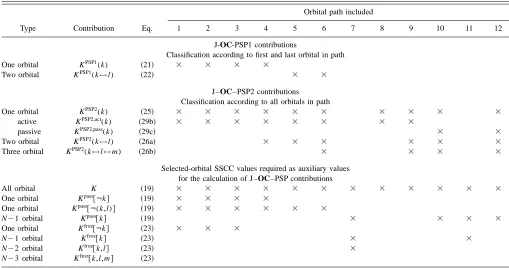
共Note that an orbital path can contribute to more than one orbital contribution in J–OC–PSP2.兲This can be clarified by considering the 12 orbital paths of Fig. 1. Paths 1, 2, and 3 are the first three members of an infinitely large set of paths defined by repeated involvement of orbital k. For example, path 2 describes how orbital k is perturbed by the spin mo-ment of nucleus B. This leads to a change in the exchange potential associated with k, which in turn changes k again by self-exchange before orbital k interacts with the spin moment of nucleus A. Hence, a path such as 1, 2, and 3 describe the self-consistent adjustment of orbital k to the perturbation provided by nucleus B. Clearly, the self-consistent adjust-ment process is of little interest for the analysis and therefore it is reasonable to sum all the corresponding path contribu-tions into a one-orbital term.

given orbital, is summed into the one-orbital contribution of this orbital, see Table I兲. All the remaining orbital terms

共third part of Table I兲 are auxiliary terms needed for the calculation rather than the analysis. The J–OC–PSP analyses

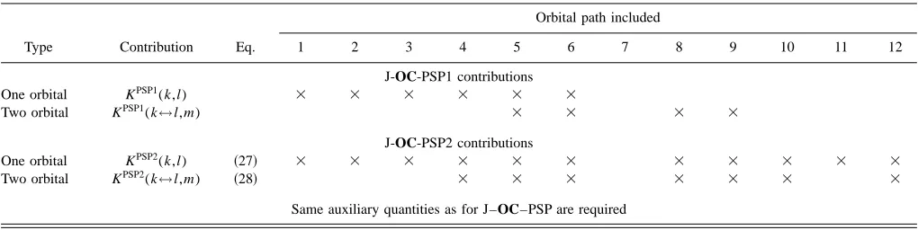
can be drastically simplified if groups of orbitals rather than individual orbitals are considered. The corresponding orbital contributions are listed in Table II.

In Table III we have summarized the orbital contribu-tions calculated by the NJC methods39,40 共classification ac-cording to the last orbital in the path; first part of Table I兲. Any analysis method that considers just the last orbital inter-acting with the responding nucleus ignores the major part of the information on the spin–spin coupling mechanism共both the active orbital at the perturbing nucleus and all interme-diate steps兲and is asymmetric with respect to the two cou-pling nuclei. In addition, any explanation must be done in terms of one-orbital contributions, which does not provide a basis to discuss the important steric exchange interactions. Therefore, we will not any longer consider terms of the type Kk used in the NJC-methods.39,40 The same applies to an analysis based on Eq.共15兲 共second part of Table III兲although such an analysis includes one-orbital terms K(k) and two-orbital terms K(k←l)and therefore should be better suited for a discussion of the electronic effects influencing the spin– spin coupling mechanism. However, any approach based on Eq.共15兲suffers from the fact that this classification is based on the last two orbitals in the path. This is chemically mis-leading and breaks the symmetry between perturbing and responding nucleus unless just one- and two-bond SSCCs are considered. Hence, we will also refrain from calculating con-tributions K(k) and K(k←l) 共see Table III兲.

[image:8.612.55.295.49.311.2]

For a decomposition of the SSCC and its Ramsey terms into one- and two-orbital terms one must use J–OC–PSP1 and calculate KPSP1(k) and KPSP1(k↔l). This analysis can be improved by obtaining active and passive contributions

FIG. 1. Selected orbital paths for spin–spin coupling between perturbing nucleus B and responding nucleus A in a three-orbital system共orbitals k, l, m兲. The paths are numbered from 1 to 12共encircled numbers兲.

TABLE I. Distribution of different orbital paths among orbital contributions as described by J–OC–PSP1 and J–OC–PSP2 for a three-orbital problem.a

Type Contribution Eq.

Orbital path included

1 2 3 4 5 6 7 8 9 10 11 12

J-OC-PSP1 contributions

Classification according to first and last orbital in path

One orbital KPSP1(k) 共21兲 ⫻ ⫻ ⫻ ⫻

Two orbital KPSP1(k↔l) 共22兲 ⫻ ⫻

J–OC–PSP2 contributions Classification according to all orbitals in path

One orbital KPSP2_{(k) 共25兲 ⫻ ⫻ ⫻ ⫻ ⫻ ⫻ ⫻ ⫻ ⫻ ⫻}

active KPSP2,act_{(k) 共29b兲 ⫻ ⫻ ⫻ ⫻ ⫻ ⫻ ⫻ ⫻}

passive KPSP2,pass_{(k) 共29c兲 ⫻ ⫻}

Two orbital KPSP2_{(k↔l) 共26a兲 ⫻ ⫻ ⫻ ⫻ ⫻ ⫻}

Three orbital KPSP2_{(k↔l↔m) 共26b兲 ⫻ ⫻ ⫻ ⫻}

Selected-orbital SSCC values required as auxiliary values for the calculation of J–OC–PSP contributions

All orbital K 共19兲 ⫻ ⫻ ⫻ ⫻ ⫻ ⫻ ⫻ ⫻ ⫻ ⫻ ⫻ ⫻

One orbital Kpass_{关¬k兴 共19兲 ⫻ ⫻ ⫻ ⫻}

One orbital Kpass_{关¬(k,l)兴 共19兲 ⫻ ⫻ ⫻ ⫻ ⫻ ⫻}

N⫺1 orbital Kpass_{关k兴 共19兲 ⫻ ⫻ ⫻ ⫻}

One orbital Kfroz_{关¬k兴 共23兲 ⫻ ⫻ ⫻}

N⫺1 orbital Kfroz_{关k兴 共23兲 ⫻ ⫻}

N⫺2 orbital Kfroz_{关k,l兴 共23兲 ⫻}

N⫺3 orbital Kfroz_{关k,l,m兴 共23兲}

[image:8.612.50.559.470.738.2]

and higher order orbital terms at the J–OC–PSP2共see Table I; at the J–OC–PSP1 level only active orbital contributions are considered兲 and thus only active orbitals can have non-zero orbital contributions, whereas orbital contributions at the J–OC–PSP2 level contain all contributions, no matter whether active or passive, of this orbital to the spin–spin coupling. In the latter case a number of auxiliary orbital con-tributions obtained in selected orbital SSCC calculations is needed to derive the actual orbital contributions KPSP2(k) and KPSP2(k↔l). Hence, for the analysis only two different types of orbital contributions共four if active and passive con-tributions must be considered兲are required whereas the cal-culations must also consider terms of the type K关k兴, K关k,l兴, etc.共see Table I兲. This comparison shows that although more than 20 different orbital contributions have been defined in this work, only a few are of importance for the actual J–OC–PSP analysis.

When applying the J–OC–PSP methods to, e.g., to the SSCC1J共CC) of ethylene, the relevant orbital contributions are KPSP1(␴(CC)) and KPSP1(␴(CH)), where at the J–OC– PSP2 level also the corresponding passive contribution of the

␲ orbital is obtained. For the simple analysis it is sufficient to handle all␴共CH兲orbitals in a single group thus reducing the number of calculations to just three. In this work, how-ever, we will further detail into individual ␴共CH兲 contribu-tions to clarify, which terms are important and which are not.

For the calculation of the auxiliary terms K关k兴, K关k,l兴, etc., given in Table I, the existing CP–DFT program16 was extended. By performing the selective orbital calculations in an order given by the equations in Sec. II A, the active and passive contributions of Table I are obtained.

D. Computational details

All SSCC calculations were carried out with the CP– DFT method described previously by us.16For this purpose, the hybrid functional B3LYP41– 43 and the basis set (11s,7p,2s/6s,2p)/关7s,6p,2d/4s,2p兴 共Refs. 44 and 45兲 de-signed for the calculation of magnetic properties was used. The SSCCs of ethylene were calculated at the experimental geometry of the molecule from Ref. 46 共bond lengths and bond angles are given in scheme 1兲.

[image:9.612.51.561.73.201.2]

The J–OC–PSP analysis and the orbital-selected SSCC calculations were carried out for LMOs obtained with a Boys localization47 where however core, ␴, and ␲ orbitals are TABLE II. Distribution of different orbital paths among orbital contributions as described by J–OC–PSP1 and J–OC–PSP2 for a three-orbital problem: Simplified version based on orbital groups.a

Type Contribution Eq.

Orbital path included

1 2 3 4 5 6 7 8 9 10 11 12

J-OC-PSP1 contributions

One orbital KPSP1_{(k,l) ⫻ ⫻ ⫻ ⫻ ⫻ ⫻}

Two orbital KPSP1_{(k↔l,m) ⫻ ⫻ ⫻ ⫻}

J-OC-PSP2 contributions

One orbital KPSP2_{(k,l) 共27兲 ⫻ ⫻ ⫻ ⫻ ⫻ ⫻ ⫻ ⫻ ⫻ ⫻ ⫻}

Two orbital KPSP2_{(k↔l,m) 共28兲 ⫻ ⫻ ⫻ ⫻ ⫻ ⫻ ⫻}

Same auxiliary quantities as for J–OC–PSP are required

[image:9.612.50.563.598.739.2]

a_{The numbering of the orbital paths refers to Fig. 1. An⫻in a table entry indicates that the orbital group contribution shown in the corresponding row includes} the orbital path given in the corresponding column.

TABLE III. Comparison with other analysis methods.a

Type Contribution Eq.

Orbital path included

1 2 3 4 5 6 7 8 9 10 11 12

Simple post-processing decomposition

Classification according to last orbital in path

One orbital Kk 共13兲 ⫻ ⫻ ⫻ ⫻ ⫻ ⫻ ⫻

Decomposition based on F˜l

(B),X

Classification according to last two orbitals in path

One orbital K(k) 共15c兲 ⫻ ⫻ ⫻ ⫻

Two orbital K(k←l) _{共15d兲 ⫻ ⫻}

Two orbital K(l←k) _{共15d兲 ⫻ ⫻}

Two orbital K(l↔k) _{共15e兲 ⫻ ⫻ ⫻ ⫻}

separately localized for reasons described elsewhere.20 All discussions are based on LMOs.

For the visualizing of the FC coupling mechanism, we will show diagrams of the FC spin density distribution

␳(B),FC_{(r) derived recently,}20

␳共B兲,FC_共r兲⫽2

兺

k occ

␺k共 0兲_共r兲␺

k 共B兲,FC_共

r兲. 共31兲

The distribution ␳(B),FC(r) can be split up into orbital con-tributions. The ␳(B),FC(r) and selected orbital contributions will be represented in form of contour line plots, where the contour levels are given by a geometric progression with the ratio of 1001/5between two subsequent contours. All SSCC calculations are performed with the ab initio program pack-ageCOLOGNE 2003.48

III. INVESTIGATION OF THE␲MECHANISM IN ETHYLENE—THE ROLE OF PASSIVE ORBITALS

In the following, we will discuss the results obtained for ethylene and unravel the role of the passive orbital contribu-tions step by step. Our focus will be predominantly on the␲ orbital and the spin information mediated by it. We will cal-culate the ␲ orbital contribution to the FC term and total SSCC.

A. The␲spin–spin coupling mechanism in ethylene

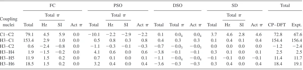
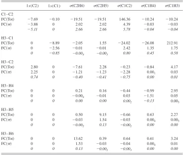
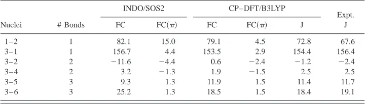
In Table IV, the calculated and measured SSCCs of eth-ylene are compared. In addition, the four Ramsey terms of the SSCCs are partitioned into active and passive ␲ contri-butions. The total ␲ contribution to each Ramsey term is given as well as the active part of this contribution. The passive ␲ contribution is obtained by deducting the active part from the total␲term. Similarly, one obtains the total␴ contributions by subtracting␲and core parts from the actual value of the Ramsey term. In Table V, the orbital contribu-tions to ␴ and␲ part, calculated according to Eq.共13兲, are listed.

The calculated SSCCs of ethylene are in reasonable agreement with the measured ones4,5共see also Refs. 33–36兲 where one has to consider that the latter must be adjusted for vibrational corrections to become directly comparable with the CP–DFT values. In this work, we are interested more in the observed trends of the SSCCs of a␲system rather than

their absolute values and in this respect the obtained agree-ment between theory and experiagree-ment is satisfactory.

Although the FC term dominates all SSCCs, the other Ramsey terms are non-negligible共Table IV兲. It is however a fact that the three noncontact terms largely cancel each other out. Therefore, we focus first on the FC coupling mechanism and the involvement of the ␲ electrons in this mechanism. Clearly there cannot be an active contribution to the FC mechanism by the ␲electrons共Table IV兲because they pos-sess zero density at the nuclei, which excludes any spin po-larization of the ␲ density by the internal magnetic field of the nucleus. However, there is a passive contribution of the␲ electrons to the FC term, which, despite the strong variation of the FC term between 0.6 and 153.4 Hz, is rather constant

共1.5 to 4.5 Hz; Table IV兲. As a result of this, the importance of the ␲part of the FC coupling mechanism increases with the length of the coupling path: For one-bond FC共CH兲 cou-pling the ␲ contribution is just 2% of the total FC term whereas for the three-bond FC terms it is more than 10%. The geminal FC terms represent an exception in so far as the magnitude of the ␲ part is comparable or even larger than that of the actual FC term and their signs differ.

In Fig. 2, the total FC spin polarization distribution关Fig. 2共a兲兴, the␲orbital contribution to the FC spin density关Fig. 2共b兲兴 and the ␲-induced part of the FC spin density in

␴共C1C2兲shown for ethylene in the y z plane, i.e., the plane cutting through the␲orbital of the molecule. The perturbing nucleus is C1 and since an␣-spin moment is assumed for the perturbing nucleus, Fermi coupling should imply a domi-nance of␤electron spin in the vicinity of C1. This is actually the case, but only in a small core region next to C1 共about 0.2 Å around C1兲not visible in Fig. 2共a兲. This core region is surrounded by a spherical region with a dominance of␣spin

关concentric solid circles in Fig. 2共a兲兴 which in turn is sur-rounded by a sphere of ␤ spin. The region around C1 is separated from a large region of␣-spin dominance surround-ing C2 by a nodal surface关Fig. 2共a兲兴.

[image:10.612.52.561.64.183.2]

The portion of the FC spin polarization that belongs to the␲共CC兲orbital is displayed in Fig. 2共b兲. This spin density is nearly identical with the spin density belonging to the J–OC–PSP2 contribution FCPSP2关␲(CC)兴 共not shown兲, i.e., the impact a freezing of the ␲ orbital has on the total spin density. In the following, we will use the notation FC共␲兲for TABLE IV. Ramsey terms, their total␲total, and their active␲contributions for all SSCCs of ethylene.a

Coupling nuclei

FC PSO DSO SD Total

Total

Total␲

Act␲ Total

Total␲

Act␲ Total Total␲ Act␲ Total

Total␲

Act␲ CP–DFT Expt.

Hz SI Hz SI Hz SI

C1–C2 79.1 4.5 5.9 0.0 ⫺10.1 ⫺2.2 ⫺2.9 ⫺2.2 0.1 0.04 0.04 3.7 4.6 2.8 4.6 72.8 67.6

H3–C1 153.4 2.9 1.0 0.0 0.5 0.8 0.3 0.8 0.4 0.3 0.3 0.1 0.4 0.1 0.4 154.4 156.4

H3–C2 0.6 ⫺2.4 ⫺0.8 0.0 ⫺1.1 ⫺0.3 ⫺0.1 ⫺0.3 ⫺0.7 ⫺0.03 ⫺0.03 0.0 0.0 0.0 0.0 ⫺1.2 ⫺2.4

H3–H4 1.9 ⫺1.5 ⫺0.2 0.0 4.1 0.6 0.0 0.6 ⫺3.8 ⫺0.1 ⫺0.1 0.3 0.1 0.0 0.1 2.5 2.5

H3–H5 11.9 1.5 0.2 0.0 0.7 0.1 0.0 0.1 ⫺1.1 ⫺0.04 ⫺0.04 ⫺0.1 ⫺0.1 0.0 ⫺0.1 11.4 11.7

H3–H6 18.5 1.5 0.2 0.0 3.2 0.4 0.0 0.4 ⫺3.6 ⫺0.3 ⫺0.3 0.3 0.4 0.0 0.4 18.4 19.1

a_{The total␲contribution is given as the sum of active共act兲and passive␲contribution. Experimental values from Ref. 35. For nuclei numbering, see scheme}

the J–OC–PSP2 contribution of the total ␲system, i.e., we will write FC instead of JFC_{and omit the superscript PSP2,}

as all orbital analyses in the present work are done at the J–OC–PSP2 level.

As the␲共CC兲orbital of ethylene has nodes at all atoms, this spin polarization is of a passive character being induced by the orbitals 1s,␴共CC兲, and␴共CH兲; similarly its impact on the responding nucleus needs to be mediated by other

elec-trons. At C1, there is a dominance of ␤spin and at C2 of␣ spin. This is also the case when considering just that part of the passive ␲contribution to the FC spin polarization trans-ported by the␴共CC兲 orbital to the responding nucleus. This part is obtained as a FC spin density difference for the␴共CC兲 orbital with the ␲共CC兲 orbital kept once unfrozen 共positive sign兲 and once frozen共negative sign兲. The spin polarization of the ␲共CC兲 orbital 关Fig. 2共b兲兴 as well as its echo on the

␴共CC兲 orbital 关Fig. 2共c兲兴, is nearly antisymmetric. Without understanding the FC spin–spin coupling mechanism, it is no longer possible to tell whether C1 or C2 is the perturbing nucleus as the spin information is transferred to the␲orbital via other orbitals rather than from the nuclear magnetic mo-ment.

Figures 2共b兲and 2共c兲suggest that the ␲ mechanism in ethylene should follow a simple pattern: From the perturbing nucleus, the spin information is coupled into the␲orbital via some ␴ orbital or chain of ␴ orbitals. The only possible reaction of the␲orbital is a polarization along the CC bond axis, and that results in a surplus of␣density in the ␲area around one of the C atoms and a corresponding ␤ surplus density at the other C atom in the bond. Hence, the values of the FC共␲兲terms should be less dependent on details of the bonding situation than the value for the total FC term.

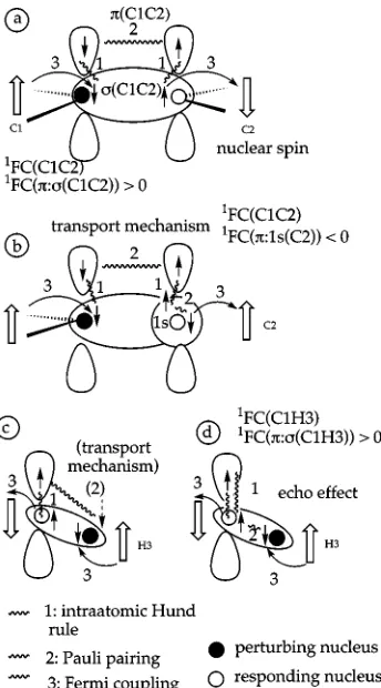
Figure 3 schematically shows the inclusion of the␲ or-bitals into the FC coupling mechanism in the case of

[image:11.612.124.486.72.378.2]

1_{J共CC). The density of the 1s(C1), ␴共C1C2兲,␴共C1H3兲, and}

TABLE V. Decomposition of the passive␲contribution to the FC term of the SSCCs of ethylene into orbitals transmitting the␲spin–spin coupling mechanism to the responding nucleus.a

1s(C2) 1s(C1) ␴共C2H6兲 ␴共C2H5兲 ␴共C1C2兲 ␴共C1H4兲 ␴共C1H3兲

C1–C2

FC共Tot兲 ⫺7.69 ⫺0.10 ⫺19.51 ⫺19.51 146.36 ⫺10.24 ⫺10.24

FC共␲兲 ⫺3.88 0 2.02 2.02 4.39 ⫺0.03 ⫺0.03

⫺5.11 0 2.66 2.66 5.78 ⫺0.04 ⫺0.04

H3–C1

FC共Tot兲 0 ⫺8.89 ⫺2.05 1.55 ⫺24.02 ⫺26.08 212.91

FC共␲兲 0 ⫺2.56 ⫺0.01 ⫺0.01 2.42 1.35 1.75

0 ⫺0.85 ⫺0.004 ⫺0.003 0.80 0.45 0.58

H3–C2

FC共Tot兲 2.80 0 ⫺7.61 2.28 ⫺0.23 ⫺0.84 4.17

FC共␲兲 2.25 0 ⫺1.21 ⫺1.23 ⫺2.28 0.001 0.03

0.74 0 ⫺0.40 ⫺0.41 ⫺0.75 0.00 0.01

H3–H4

FC共Tot兲 0 0 0.21 0.16 ⫺0.44 ⫺0.99 2.95

FC共␲兲 0 0 ⫺0.004 ⫺0.01 0.03 ⫺1.51 0.05

0 0 0.00 0.00 0.002 ⫺0.13 0.003 H3–H5

FC共Tot兲 0 0 0.50 9.15 ⫺0.66 0.63 2.27

FC共␲兲 0 0 ⫺0.03 1.54 ⫺0.03 0.004 0.003

0 0 ⫺0.002 0.13 ⫺0.002 0.00 0.00

H3–H6

FC共Tot兲 0 0 13.62 0.39 0.64 0.61 3.24

FC共␲兲 0 0 1.53 ⫺0.03 ⫺0.04 0.004 0.01

0 0 0.13 ⫺0.002 ⫺0.003 0.00 0.00

a_{For nuclei numbering see Scheme 1. The nucleus given first is the perturbing nucleus. Italicized numbers are}

reduced SSCCs in SI units of 1019_{J T}⫺2_{, all others are in Hz. CP–DFT/B3LYP/(11s,7p,2d/5s,1p)}

⫻关7s,6p,2d/4s,2p兴calculations.

␴共C1H4兲orbital is spin polarized by the perturbing nucleus C1 by Fermi coupling 关Fig. 3共a兲, mechanism 3兴 in the way that the spin density close to C1 is dominated by␤spin. The spin-polarized␴ density causes also a dominance of␤ spin in the␲orbital at C1 according to the intra-atomic Hund rule

共mechanism 1兲. Pauli coupling 共mechanism 2兲 of the elec-trons of the␲bond leads to a dominance of␣spin at nucleus C2, which of course does not affect the spin of nucleus C2, however the C2 surrounding␴density is affected in the way that this also is preferentially of␣spin共mechanism 1兲. The

␴-spin density leads to a ␤-spin moment of nucleus C2

共Fermi coupling, 3兲and a positive␲contribution of 4.4 Hz, i.e., by this amount the FC coupling mechanism transmitted through the ␴共CC兲-spin density 共142 Hz, Table V兲 is in-creased.

The external CH bonds all lead to a negative ␴ contri-bution to1FC共CC)共⫺21.5 and⫺10.2 Hz, Table V兲, which is typical of one-bond coupling constants and has been dis-cussed in Ref. 20共the one-bond path is extended to a two-bond coupling path thus implying a change in sign兲. At the

site of the responding nucleus C2, there are passive ␲ con-tributions of 2.0 Hz 共Table V兲 caused by a transmission of the ␲-spin polarization to the␴共C2H5兲- and ␴共C2H6兲-spin density. Since the mechanism via the ␲-orbital functions in the same way as described in Fig. 3共a兲, the contribution is positive, although somewhat smaller than for ␴共C1C2兲 con-sidering the fact that the CH LMOs have smaller amplitudes at the responding nucleus.

A relatively strong passive␲contribution of⫺3.9 Hz is obtained via the 1s core orbital at C2. This change in sign and the FC spin density pattern at C1 are related. The 1s orbital is fully localized in the core region of C2. If the electron in the outer sphere of the 1s(C2) orbital adopts preferentially␣spin because of the spin-polarization mecha-nism via the ␲ orbital 关Fig. 3共b兲兴, the ␤ 1s electron must contract toward the C2 nucleus and generate a surplus of ␤ spin there关Fig. 3共b兲兴, as␣and␤electron always respond in an opposite way to the FC perturbation. Fermi coupling leads to an ␣nuclear spin and accordingly to a negative 1s(C2) contribution of the passive␲part.

The electron pair in the 1s(C1) orbital is spin polarized in the opposite way共␤spin close to the nucleus;␣spin in the outer sphere of the 1s orbital兲 as can be seen in Fig. 3共b兲. This spin distribution is superimposed by that of the s p2

hybrid orbital forming the CC ␴bond, which is completely negative 共␤ dominated兲in the region of C1 but positive 共␣ dominated兲 in the region of C2 again due to the opposite response of ␣ and ␤ electron, which is enhanced by ex-change effects and left–right correlation. Figure 2共a兲shows that in the 共outer兲core region of C1 the spin polarization of 1s共dominance of␣兲, in the valence region the spin polariza-tion of the s p2 hybrid orbital dominates共dominance of␤兲.

The passive␲contributions to the FC term of1_J共C1H3)

can be explained in the same way if one considers that the

␴-bond density C1H3 is anisotropic共because of the ␲ den-sity at C1兲 rather than rotationally symmetric. In the quan-tum chemical calculation, this can only be correctly de-scribed by the inclusion of p-type polarization functions at the H atom. Hence, there is a ␲-type contribution to reflect the anisotropy of the C1H3 bond density. In Figs. 3共c兲 and 3共d兲, this is schematically indicated where Fig. 3共c兲indicates the ␲-type mechanism similar to the case of 1J共CC) 关Fig. 3共a兲兴and Fig. 3共d兲describes an echo effect: spin polarization is transmitted via the␴共C1H3兲-orbital to nucleus C1共H3 is the perturbing nucleus兲. There it causes the spin polarization of the ␲ density at C1, which can in turn increase the spin polarization of any s-type density close to the nucleus C1.

Clearly, the␲effects for the1FC共CH) coupling mecha-nism are smaller than those of the1FC共CC) one as there are no real p orbitals at the H atom. However, both the type and the relative ratio of positive and negative␲contributions are the same so that the calculated value of 2.9 Hz reflects again the partial cancellation of positive valence共2.4, 1.7, 1.4 Hz, Table V兲and the negative core contribution共⫺2.8 Hz兲.

[image:12.612.89.261.49.359.2]

All passive␲-contributions to the orbital terms listed in Table V can be explained in a similar way. Only those orbit-als with a sizable amplitude at the responding nucleus lead to a significant contribution. For example, for the C1C2 cou-pling, these are the ␴共C1C2兲, ␴共C2H5兲, ␴共C2H6兲, and the

FIG. 3. FC coupling mechanism in ethylene involving the passive␲orbital.