Determination of the Fundamental Image Categories for Typical Consumer Imagery

Rochester Institute of Technology

RIT Scholar Works

Theses

Thesis/Dissertation Collections

2007

Determination of the Fundamental Image

Categories for Typical Consumer Imagery

Kenneth N. Fleisher

Follow this and additional works at:

http://scholarworks.rit.edu/theses

This Thesis is brought to you for free and open access by the Thesis/Dissertation Collections at RIT Scholar Works. It has been accepted for inclusion in Theses by an authorized administrator of RIT Scholar Works. For more information, please [email protected].

Recommended Citation

Determination of the Fundamental Image Categories

for Typical Consumer Imagery

Kenneth N. Fleisher

B.F.A. Rochester Institute of Technology

(1989)

A thesis submitted in partial fulfillment of the requirements

for the degree of Master of Science in Color Science

in the Chester F

.

Carlson Center of Imaging Science of the College of Science

Rochester Institute of Technology

September 2007

Kenneth N. Fleisher

Signature of the Author

Roy S.

Berns

Accepted by Dr. Roy S. Berns

CHESTER F

.

CARLSON CENTER FOR IMAGING SCIENCE

COLLEGE OF SCIENCE

ROCHESTER INSTITUTE OF TECHNOLOGY

ROCHESTER

,

NEW YORK

CERTIFICA TE OF APPROVAL

M.S. DEGREE THESIS

The M.S. Degree Thesis of Kenneth N. Fleisher

has been examined and approved by two members of the color science faculty

as satisfactory of the thesis requirement for the Master of Science Degree

Mark D. Fairchild

Dr. Mark D. Fairchild

Roy S.

Berns

CHESTER F. CARLSON CENTER FOR IMAGING SCIENCE

COLLEGE OF SCIENCE

ROCHESTER INSTITUTE OF TECHNOLOGY

ROCHESTER, NEW YORK

THESIS REPRODUCTION PERMISSION STATEMENT

Title of thesis

:

Determination of the Fundamental Image Categories for Typical

Consumer Imagery

I, Kenneth N. Fleisher, hereby

grant permission

to the Wallace Library of the Rochester

Institute of Technology to reproduce my thesis in whole or in part. Any reproduction will

not be for commercial use or profit.

Kenneth N. Fleisher

Signature of the Author

Determination

of

the

Fundamental

Image Categories

for Typical

Consumer

Imagery

Kenneth N. Fleisher

B.F.A. Rochester Institute of

Technology

(1989)

ACKNOWLEDGEMENT

Iwouldliketoextend_mysincerestthankyoutoDr. Ethan D.

Montag

for hisguidance on thisproject andfor

helping

metolearna greatdealabout psychophysics.

Iwould alsoliketo thankDr.

Roy

S.

Berns,

Dr. Mark D. Fairchild,and everyoneatthe

Munsell Color Science

Laboratory

for

helping

tomake_my

journey

incolor science a

truly

memorableexperience.

A specialthanks toDave WybleandLawrence Taplinfortheir

help

withtheDistributed

Experimentandto

Li, Willy, Iris, Mahnaz,

andMahdi for

listening

toand

helping

me with an endlessamountof random questions about color science.

Thisresearch was supported

by

a grantfromLexmark

International,

Inc. Iwantto thank

Ann

McCarthy

andBrant Nystrom from Lexmarkfor makingthis_opportunitypossible.

Determination

of

the

Fundamental

Image Categories

for

Typical Consumer

Imagery

Kenneth N. Fleisher

B.F.A. Rochester Instituteof

Technology

(1989)

Athesissubmittedinpartialfulfillmentoftherequirements

forthedegreeofMasterofScience in Color Science

intheChester F. Carlson Centerof

Imaging

ScienceoftheCollegeofScience

Rochester Instituteof

Technology

ABSTRACT

Many

tasks in

imaging

science are image-dependent. While a particular

dependency

might _{simply be} a function of certain physical attributes ofan

image,

often it is _closely relatedto theperceivedsemantic category.

Therefore,

athorough_{understanding}ofimage semanticswouldbe ofsubstantial practical value. _{The primary}goal ofthisresearch was to determine the fundamental semantic categories for typical consumer imagery. Two

psychophysical experiments were performed. Experiment I was a Free

Sorting

Experimentwhere observerswere asked tosort 32 1 images into piles of similarimages.

ExperimentII wasa Distributed Experimentconducted overthe internet which usedthe

method oftriadsto collect similarityand

dissimilarity

data from 321 images. Due to the

largenumber ofimages included in the experiment, themethod of_{non-repeating} random

paths wasemployedtoreducethe numberof required responses. Bothexperiments were

analyzed _using multidimensional _scaling and hierarchical cluster analysis. The Free

Sorting

Experiment was also analyzed _{using dual} scaling. The results from all three methodswere compiled andasetof34categoriesthatprovedtobe stable acrossmultiple methods of analysis was formed. A multidimensional perceptual image semantic space has been suggested andadvantages to_utilizing such a structurehave been outlined. The

34 fundamental categories were represented

by

10perceptual dimensions that

described

the _underlying perceptions

leading

to categorical assignments. The 10 perceptual

dimensions were

humanness,

artificialness, perceived_{proximity, candidness,}

wetness,

TABLE OF CONTENTS

1. INTRODUCTION 1-1

2. EXPERIMENTAL 2-1

2.1 IMAGESELECTIONPROCESS 2-1

2.1.1

Category

Selection 2-1

2.1.2 ImageSelection 2-5

2.2 IMAGE PREPARATION 2-6

2.3 EXPERIMENT I FREESORTING EXPERIMENT 2-8

2.3.1 Observer Statistics 2-9

2.4 EXPERIMENTII DISTRIBUTED EXPERIMENT. 2-9

2.4.1 Experimental Design 2-9

2.4.2 Experiment Interface 2-12

2.4.3 Observer Statistics 2-15

2.4.4

Pre-Filtering

Observer Responses 2-16

3. METHODSOF ANALYSIS 3-1

3.1 MULTIDIMENSIONALSCALING 3-1

3.1.1 Goodness-of-Fit 3-3

3.1.2

Dimensionality

3-5

3.1.3 Configuration 3-6

3.2 DUAL SCALING 3-7

3.3 HIERARCHICAL CLUSTER ANALYSIS 3-11

3.3.1 Agglomerative Hierarchical Methods 3-12

3.3.2 Divisive Hierarchical Methods 3-12

3.3.3 Linkage Methods 3-13

3.3.4 Interpretation oftheCluster Tree 3-15

3.3.4.1 Cophenetic Correlation Coefficient 3-15

3.3.4.2 Dendrogram 3-16

3.3.5 Cluster Interpretation 3-19

4. DATAPREPARATION 4-1

4.1 EXPERIMENTI FREESORTINGEXPERIMENT 4-1

4.2 EXPERIMENTII DISTRIBUTED EXPERIMENT. 4-2

5. DATA ANALYSIS 5-1

5.1 MULTIDIMENSIONAL SCALING 5-1

5.2 DUALSCALING 5-3

5.3 HIERARCHICAL CLUSTER ANALYSIS 5-4

6. GOODNESS-OF-FIT 6-1

6.1 MULTIDIMENSIONALSCALING 6-1

6.2 HIERARCHICAL CLUSTER ANALYSIS 6-3

7. DIMENSIONALITY 7-1

8. CLUSTER INTERPRETATION 8-1

8.1 2-DIMENSIONAL MULTIDIMENSIONALSCALING 8-1

8.2 3-DIMENSIONAL MULTIDIMENSIONAL SCALING 8-5

8.3 DUALSCALING 8-10

8.4 HIERARCHICAL CLUSTERANALYSIS 8-12

8.5 LOCAL MULTIDIMENSIONAL SCALING CONFIGURATIONS 8-16

8.6 FINAL FUNDAMENTAL CATEGORIES 8-24

9. DISCUSSION 9-1

9.1 COLOR PERCEPTION. 9-1

9.2 PERCEPTUALIMAGESEMANTICDIMENSIONS 9-2

9.3 PERCEPTUALDIMENSIONDEFINITIONS 9-7

10. SUMMARY 10-1

10.1 CONCLUSIONS 10-1

APPENDIX A Final 321 ImagesSelected forPsychophysicalExperiments A-l

APPENDIXB Sheppard Diagrams fortheDistributed Experiment B-₁

APPENDIXC Silhouette Plots C-l

APPENDIXD Three-DimensionalMultidimensional

Scaling

Configurations D-₁

APPENDIXE Dual

Scaling

Dimension Extremes E-l

APPENDIX F Heirarchical Cluster Analysis Free

Sorting

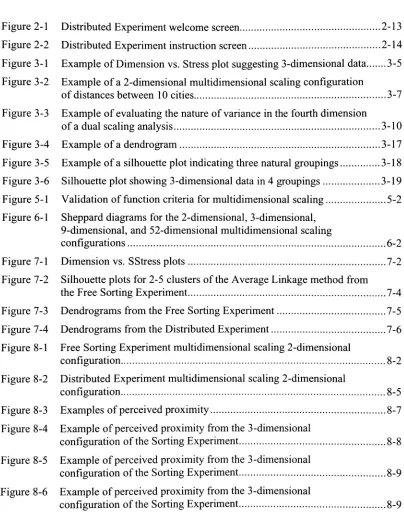
Experiment F-₁

LIST OF

FIGURES

Figure2-1 Distributed Experimentwelcomescreen 2-13

Figure 2-2 Distributed Experiment instructionscreen 2-14

Figure 3-1 ExampleofDimensionvs.Stressplot_{suggesting 3-dimensional}data 3-5

Figure 3-2 Exampleof a2-dimensionalmultidimensional_scalingconfiguration

ofdistances between 10 cities 3-7

Figure3-3 Exampleof_evaluatingthenature ofvarianceinthefourthdimension

of adual_scalinganalysis 3-10

Figure 3-4 Exampleof adendrogram 3-17

Figure3-5 Exampleof a silhouette plot

indicating

threenatural groupings 3-18

Figure3-6 Silhouetteplot_{showing 3-dimensional data in 4}groupings 3-19

Figure5-_{1 Validation offunctioncriteriaformultidimensional}

scaling 5-2

Figure6-1 Shepparddiagramsforthe

2-dimensional, 3-dimensional,

9-dimensional,

and52-dimensionalmultidimensional_scaling

configurations 6-2

Figure 7-1 Dimensionvs. SStressplots 7-2

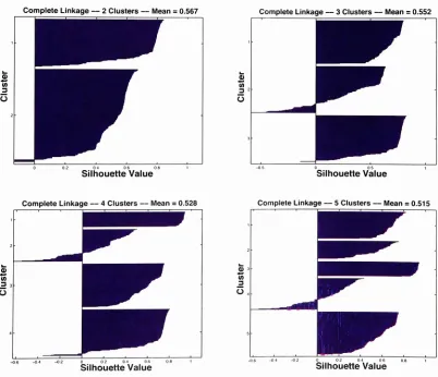
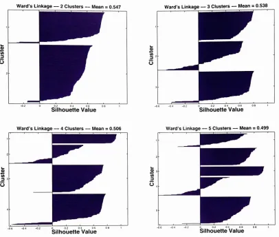
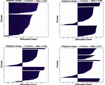
Figure 7-2 Silhouetteplotsfor 2-5 clusters oftheAverage Linkagemethodfrom

theFree

Sorting

Experiment 7-4

Figure 7-3 DendrogramsfromtheFree

Sorting

Experiment 7-5 Figure 7-4 Dendrograms fromtheDistributed Experiment 7-6 Figure8-1 Free

Sorting

Experimentmultidimensional_scaling2-dimensional

configuration 8-2

Figure8-2 Distributed Experimentmultidimensional_{scaling 2-dimensional}

configuration 8-5

Figure8-3 Examplesofperceived_proximity 8-7

Figure8-4 Exampleofperceived_proximityfromthe3-dimensional

configurationofthe

Sorting

Experiment 8-8

Figure 8-5 Exampleofperceived_proximityfromthe3-dimensional

configurationofthe

Sorting

Experiment 8-9

Figure8-6 Exampleofperceived_{proximity from}the3-dimensional

[image:10.511.56.460.103.627.2]

Figure 8-7 Imagesattheextremesofdimension 1 anddimension2 from dual

scalinganalysisfortheFree

Sorting

Experiment 8-10

Figure 8-8 Cluster interpretations fromhierarchicalcluster analysis 8-15

Figure 8-9 Multidimensional_{scaling 2-dimensional} configurationfortheFree

Sorting

Experiment.Imagesare coloredbasedonthe 6-cluster

grouping usingtheweightedlinkagemethod ofhierarchicalcluster

analysis 8-17

Figure 8-10 _{Multidimensional scaling 2-dimensional}configurationforthe

DistributedExperiment. Imagesare coloredbasedonthe6-cluster

grouping usingtheWard'slinkagemethod ofhierarchicalcluster

analysis 8-18

Figure 8-1 1 _{Multidimensional scaling 2-dimensional}configurationfortheFree

Sorting

Experiment. Imagesare coloredbasedonthe6-cluster grouping usingtheweightedlinkagemethod ofhierarchicalcluster

analysis. Localmultidimensional_scalingwasappliedtoimage

groupingswithineach circle.Thecircle centers arethecentroids

fromthe_{corresponding hierarchical}clusteranalysis clusters 8-19

Figure 8-12 Multidimensional scaling 2-dimensionalconfigurationforthe Distributed Experiment. Imagesare coloredbasedonthe6-cluster

grouping usingtheWard'slinkagemethodofhierarchicalcluster analysis. Localmultidimensional_scalingwasappliedtoimage

groupingswithineach circle. Thecircle centers arethecentroids

fromthe_{corresponding hierarchical}clusteranalysis clusters 8-20

Figure8-13 Localmultidimensional_{scaling 2-dimensional}configurationforthe

Free

Sorting

_{Experiment using images}fromwithin circle#2

(green)

in Figure8-10 8-21

Figure 8-14 Localmultidimensional_{scaling 2-dimensional}configurationforthe

Free

Sorting

_{Experiment using}images fromwithincircle#3

(blue)

inFigure 8-10 8-22

Figure A-l Final321 images selectedforuseinthepsychophysicalexperiments A-l

Figure B-l Sheppard diagramsforthe

2-dimensional,

3-dimensional,

9-dimensional,

and52-dimensionalmultidimensional_scaling

configurations B-l

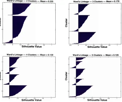
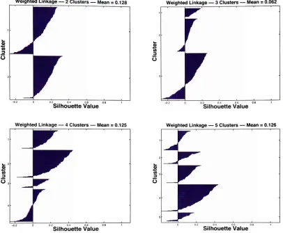
FigureC-_{1 Silhouetteplotsfor2-5} clustersfortheFree

Sorting

Experiment C-l

FigureC-2 Silhouetteplotsfor2-5 clustersfortheDistributedExperiment C-4

Figure D-l Three-dimensionalmultidimensional_scalingconfigurationforthe

Figure D-2 Three-dimensional multidimensional_scalingconfigurationforthe

Distributed Experiment D-ll

FigureE-_{1 Imagesatthedimensional}

extremesfortheFree

Sorting

Experiment E-l FigureE-2 Imagesatthedimensionalextremesforthe DistributedExperiment E-3 Figure F-l Hierarchical Cluster_{Analysis 5-Cluster division using}theaverage

linkagemethodfortheFree

Sorting

Experiment F-l Figure F-2 _{Hierarchical Cluster Analysis 6-Cluster division using}theaverage

linkagemethodfortheFree

Sorting

Experiment F-8 FigureG-l Localmultidimensional_scaling2-dimensionalconfigurationforthe

Free

Sorting

_{Experiment using}imagesfromwithinclustergroupings

in Figure 8-10 G-l

Figure G-2 Localmultidimensional_scaling2-dimensionalconfigurationforthe Distributed Experiment usingimages fromwithin clustergroupings

LIST OF TABLES

Table 2-1 Categories fromprevious studies 2-3

Table 2-2 Finalcategoriesused as a criteriaintheimageselection process 2-4

Table2-3 Totalnumber of required observationsforn samples 2-11

Table 2-4 Metadatacollected

during

Distributed Experiment 2-15

Table 2-5 ObserverstatisticsfortheDistributed Experiment 2-16 Table 3-1 Goodness-of-Fit "ruleofthumb"forstressvalues 3-3

Table6-_{1 Copheneticcorrelationcoefficientforthesevenlinkage}methods 6-4

Table 8-_{1 Categories resultingfromdual scalinganalysis oftheimagesatthe}

extremes ofthe dimensions 8-12

Table 8-2 _{Categories resulting from interpretation}of2-dimensional local

multidimensional_scalingconfigurations 8-23

Table8-3 Finallistoffundamentalcategories_resultingfrombothexperiments

andall methodsof analysis 8-25

semantics, si-man'tiks, _{The study} ofmeanings. The termis derived throughGreek "semainein"

("to signify"

or "to

mean"). Itisconcernedwiththerelationbetween words

or other symbols and the objects or conceptsto which

they

refer, as well as withthe

history

ofmeanings and

the changes

they

undergo.

(Semantics,

2001)

1. INTRODUCTION

The term semantics refers to the aspects of _meaning that are expressed in a

language. Photographic images tend to be perceived as

belonging

tobroad categories of

images such as human portraits,

landscapes,

sports, animals, etc. These categorical

identifiers are referred to as image semantics language that is used to describe the

meaningofpictorialcontent.

Many

tasks in

imaging

science are image-dependent. While a particular

dependency

might _simplybeafunctionof certain physicalattributes of an

image,

oftenit

is _closely related to the perceived semantic category.

Therefore,

a thorough

understanding ofimage semantics would be of substantial practical value. _{For example,}

there are _many

imaging

tasks where image dependencies can influence the results of a

certain _processing task. Gamut mapping,

halftoning,

contrast _adjustment, and

compression are alldependantonthe typeofimage

being

processed.

Additionally,

_image

quality judgments have been shown to exhibit image dependencies

(Montag

and

Kasahara,

2001). If one could determine in advance what type of image was

being

processed, thenan appropriateset of_processing parameterscouldbe selected so that the

Before one can

identify

which fundamental image category a particular image

belongs to, it is necessary to determine what those categoriesare. There has been a lot

work in the area of automatic image classification

(Wardhani,

2003; Lee,

et al.,

2005;

Le

Borgne,

et _al., 2003).

However,

most of these methods _rely on

finding

image

descriptors thata machine can discriminate.

Unfortunately

thesesamedescriptors are not

necessarily perceptually significant. The

difficulty

lies in the fact that low-level image

descriptorssuchas color and contrastfailtocaptureimportantsemantic

information,

lack

fine

discrimination,

and do not tend to match human perception

(Moj

silovie,

Hu,

&

Soljanin,

2002). Another concern is related to the basic goal of automatic image

classification. "Classificationpertains toa known number of_groups, and the operational

objective is toassign new observations to one ofthese groups."

(Johnson and

Wichern,

2002,

p. 668). The problem here is that the fundamental groups, or _categories, are not

known and are _simply selected

by

researchers based on a wide range of inconsistent

criteria.

There is a

body

of work that addresses the problem of _{correlating image}

semantics with machine discernable image descriptors

(Depalov,

et _al,

2006;

Iqbal and

Aggarwal, 2002;

Le

Borgne,

etal.,

2003; Lee,

et_al.,

2005;

Mojsilovicand

Gomes, 2002;

Mojsilovic and

Hu,

2000; Mojsilovic, Hu,

&

Soljanin, 2002;

Mojsilovic and

Rogowitz,

2001a; Serrano,

et_al.,

2002)

but work inthis area isnot extensive.

Further,

justas there

are image

dependencies,

it has been shown that _any set of

fundamental

semantic

categories that are determined will be influenced

by

the image genre

(Laine-Hernandez

dependent on what images were used in the _study and images from different areas of

photographywill exhibitdifferent fundamentalcategories.

Besides_using semantic categoriestooptimizeimage processingalgorithms, there

are other ways this information canbe utilized. Imageretrieval from large databases of

images is a significant problem andtechniques thatcan

help

theuser

identify

the image

they

are

looking

formore _quickly can _greatly improve the process. Much ofthe image

classification researchhasbeenorientedtoward_solving thisproblem

(Chen,

et_al.,

2005)

(Cox,

et_al.,

2000; Chen,

et_al.,2003).

Unfortunately,

much ofthiswork doesnot

directly

addresstheproblem offirst

identifying

thesemantic categories thattheimages shouldbe

divided into.

Instead,

categories are selected based on either intuition or the ease of

relating the image to low-level descriptors. Little or no regard for the perceptual

significance ofthecategories isconsidered.

Another usefor semantic image categoriesis image qualityresearchinwhichthe

results canbeshowntobe image dependent. Becausethe _{image qualityresulting from}an

image processing algorithm or an

imaging

system will depend on the image

being

evaluated, it would be _very useful to know in advance what the fundamental image

categoriesare. Althoughthisissue isnotunknown_{to researchers,}most oftenthe solution

is topick a _variety ofimages _arbitrarily to include in an experiment or study. There are

twopotential problems withthisapproach.

First,

it ispossible that thereare wholeimage

classes thathave been

inadvertently

leftout ofthe study

thereby

makingthe results less

comprehensivethandesired. Thesecondprobleminvolves

including

multiple

images

that

could result in extra work

(particularly

in collecting the

data)

which would not produce

any additional information.

Therefore,

by knowing

in advance the fundamental image

categoriesforaparticular_application, one canbe surethat

they

are

testing

the fullrange

of possibleimagetypeswithout_{unnecessary duplication}ofeffort.

By identifying

the fundamental image categories for aparticular_application, one

can _apply this knowledge to

develop

optimized image _processing algorithms, better

2.

EXPERIMENTAL

The _primary goal of this research was to

identify

the fundamental image

categories for typical consumer

imagery

(snapshots). To achieve this _goal, two

psychophysical experiments were conducted. Experiment I was a Free

Sorting

Experiment and ExperimentII was aDistributed Experimentwhich wasconducted over

theinternet.

2.1 IMAGE

SELECTION

PROCESS

The design of both psychophysical experiments began with image selection.

Because the same set of images was used for both experiments and because the

usefulnessoftheexperimental results isdependentontheimages selectedfor inclusionin

the studies, a greatdealof care wastaken toensurethat theimageswere representative of

the intended application and that

they

spanned a wide gamut across potential image

categories. There is an inherent

difficulty

in this processbecause it is _necessary to first

make categorical judgments in order to select a range of images for the _studies, but

determining

categoricaljudgments is_preciselythe objective oftheresearch. Therefore it

was_necessarytoapproachimageselectionwiththemost objective methodspossible.

2.1.1

Category

Selection

Without

knowing

the image categories inadvance, how does one

determine

that

the widest range of categories are _properly represented and how does one avoid

make use of results fromprior studies as a _startingpoint. An extensive list of semantic

categories was compiled from _many sources (Mojsilovic and

Rogowitz,

2001b;

Wardhani, 2003;

Wardhaniand

Thomson, 2004; Oldfield, 2005;

Rogowitz,

etal.,

1998)

and is listed in Table 2-1. There were _manystudies investigated thatare not included in

Table

2-1,

however the categories that were identified in those studies were _already

represented and _therefore, therewasno needtoreport redundantinformation. Categories

thathad been_{previously identified}

by

other researchersbutwere notconsidered semantic

categories such as shape dominant and geometric objects were not included in the

final _category selection. Thisisjustified because the categories thatwere excluded were

originallyidentifiedtorepresentobjectsdescribed

by

variouslow-level image descriptors

that were calculatedfrom the test imagesratherthan to represent image semantics. Also

excluded were _any categories that could not be considered typical consumer

imagery

such as product _photography and artificial scenes (i.e. graphics). The final list of

[image:20.511.54.460.102.611.2]

TABLE 2-1:

Categories

fromprevious studies.

STUDY1 STUDY2 STUDY3 STUDY4 STUDY 5 STUDY 6 STUDY7

Portraits Landscape Natural Scene Manmade People

High-Frequency Animals

People

Outdoors People People Natural Non-People

Low-Frequency People

People Indoors Shape Dominant

Geometric Shapes

MoreHuman

like General Occasion Color Indoor Scenes

OutdoorScenes

withPeople

Color

Dominant Single Object

Less Human

like Vacation HighKey Nature Crowdsof People Texture Dominant Multiple Objects Special Days (Birthdays, Celebrations)

Low_Key Buildings

Cityscapes Structure

Dominant MainlySmooth Weddings Textures

Outdoor Architecture

Mainly

Textural Holidays Manmade

Technoscenes Recreation,

SportingEvents

Objects Indoors SubjectDistance

<10ft. Waterscapes withHuman Influence SubjectDistance 10-30ft.

Waterscapes Subject Distance

>30ft.

Landscapes

withMountains Outdoors

Sky/Clouds Indoors

Winter/Snow ElectronicFlash

Green

Landscapes Sunlight/Daylight

Landscapes

withFieldsand

Foliage Cloudy Day Plants, Flowers, Fruits, andVegetables Dawn/Dusk

Animals Indoor Natural

TABLE 2-2: Final categories used as a criteria in the image selection process.

Categoriesfor Image Selection Process

Portraits

PeopleOutdoors PeopleIndoors

Outdoor SceneswithPeople CrowdsofPeople

Cityscapes

Outdoor Architecture Objects Indoors Objects Outdoors

Waterscapes

WaterscapeswithHuman Influence LandscapeswithMountains

LandscapeswithFieldsandFoliage GreenLandscapes

LandscapeswithWater Sky/Clouds

Winter/Snow

Plants,

Flowers, Fruits,

andVegetables Animals

Textures, Patterns,

andClose-ups General Occasion

Vacation

Special Days

(Birthdays, Celebrations,

etc.) Weddings

Holidays Recreation

2.1.2 Image Selection

There werefourcriteria usedintheimageselection process. Thesewerebasedon

criteria identified from prior work and were determined to be a reasonable guide for

imageselection.

They

fourcriteria usedwere:

1)

Widerange _ofcategories For each _{category listed in Table}

2-2,

images were

selected such that each _categorywas represented

by

a minimum offour images.

Naturally,

therewas an inherent _overlapand some imagescouldbeconsideredto fill therequirements formore than one category. For example,ifone_category is people outdoors and anotherisnaturescenes, then animageofapersoninnature could fulfill the requirement for both categories.

Many

categories were represented

by

fargreaterthanfourimages.

2)

Camerazoom Foreach _category,a rangeof_{wide-angle, normal,} and_close-up

imageswereincluded.

3)

Image orientation A distribution of landscape and portrait orientation was

included foreach ofthecategories.

4)

Color A broad range of color and lightness levelswas included. These were

determined

by

_examining average CIELAB values for each

image,

which was

calculated as a simple average of_everypixel color. Carewastaken to includean evendistribution inallthreedimensions

L*,

_a*,andb*.

The images were obtained from a _variety of sources. Most ofthe images in the

final selection were supplied

by

Lexmark

International,

Inc. A

library

of_{nearly 1,000}

images were

initially

provided. Despite this large number of

images,

there was not

enough _{variety among} them to _satisfy all four selection criteria. _{After pre-editing} the

remaining images were obtained from the Corel Image Database and from the Munsell

Color Science Laboratory. For example, after ananalysis ofaverage CIELABvalues for

theselected

images,

itwasdeterminedthat therewereno_{very light images}which wasan

indication that pictures with snow were missing.

Therefore,

a _variety of snow images

were addedfromtheCorelImage Database.

A total of321 images were included in the final selection. The complete set of

321 images can be found in Appendix A. To the experienced scientist, this may seem

alarming since the typical number of images included in this type of _study is usually

closerto 100 orfewer. Thereason for _usinga smaller number ofimages is

because,

for

manyexperimental

designs,

as thenumber of samples

(images) increases,

thenumber of

required observations increases rapidly. This generally makes a sample size of 321

infeasibleto workwith. The experimental design forthe Distributed Experiment (which

wouldbemore sensitive tosample sizethan the Free

Sorting Experiment)

wastaken into

consideration while

deciding

on thenumber ofimages toinclude. Thedetails ofhowthe

experimentaldesignwouldeffect selectionof a sample sizeis describedinsection2.4.1.

2.2 IMA GE

PREPARA

TION

The321 test imageswereobtainedfroma_varietyof sources. Someofthe images

weretaggedwithan ICCprofile, but manywere not. Forthis_reason, the imagesneeded

to beadjusted in ordertopresent a consistent appearance to the observers. _ExperimentI

requiredprintedoutput oftheimagesandExperiment IIrequiredthe

images

tobeviewed

sRGB color space.

Therefore,

all test images were adjusted so that

they

produced a

pleasing imagewhile viewedinthesRGB colorspace.

The firsttaskwastocharacterize themonitor onwhich

they

would be evaluated.

This was accomplished _using

industry

standard calibration hardware and software. An

Apple LCD

display

was calibrated _using a GretagMacbeth EyeOne Pro

spectrophotometer and GretagMacbeth ProfileMaker Pro software version 5.0. Images

were viewedinAdobe Photoshop. A Lexmarkinkjetprinterwasusedtomake prints.The

printer was characterized _{using ProfileMaker Pro} and a GretagMacbeth Spectrolino

Spectroscanspectrophotometer.

Ifan imagewas untagged, it was assigned the sRGB profile. Ifthe image was

taggedwith_somethingother_{than sRGB, then}itwas convertedto sRGB. All imageswere

then adjusted,whennecessary, sothat

they

produced a_pleasingappearance while viewed

under the conditions specified

by

sRGB. Since the objective of this _study was not

dependent on specific colors in the

images,

it was not _necessary to ensure exact color

reproduction. The purpose for _{setting up} color management and _performing color

adjustments was_simplytonormalize theappearance ofimages froma_varietyofsources.

Onceallimageswere_adjusted,

they

werescaledtoa common sizeappropriatefor

theinternet(200pixels ontheshortdimensionand300pixels onthe

long

dimension)

and

savedintheJPEGformat_usinglow compression

(Photoshop

level 1

0)

which yieldedfile

sizes_ranging from52KB to 120 KB. Some images were adifferent dimension and were

printer at a size of4x 6 inches.

Finally,

theimagesweretrimmedandnumberedwithbar

codes onthebacktoaidthedatacollection process.

2.3 EXPERIMENT

I

FREE

SORTING

EXPERIMENT

The first experiment was a

tabletop

_sortingexperiment. Observers were asked to

sortthe321 testimages intopilesthatrepresented categories.

They

were freetocreate as

few or as _many piles as

they

felt _necessary to _properly represent the categories.

They

were also free to change their mind and rearrange images in the piles as needed. Exact

instructions as to how to categorize the images were not provided. The instructions

providedtotheobservers read asfollows:

You will be given a stack of 321 4x6 photographic prints. Your task is to sort these into piles that represent different categories ofimage types. _{You may decide}

by

what criteria to separate the images into categories and you _may create as_manypiles

(categories)

as you feelarenecessary.

Ifaparticularimage seems appropriate formore than one _category that you have

defined,

then use whichever

identifying

featureyou feel is the_primary

feature,

or create a new category. Ifyou create a new_category, remember to go through theimages that_{have already been} sortedtoseeif any ofthose

belong

to thenew category.

After youare

finished,

you willbe asked tocomplete one additional smalltask.

After the observers completed the task ofseparating the images into piles,

they

were askedto writedown what criteria

they

usedto separate the imagesinto categories.

Finally,

the observers were asked to name the categories thatrepresented each pile that

they

made.

2.3.1 Observer Statistics

Thirty (30)

observers participated inthe _sorting experiment ofwhichtherewere

19 males and 11 females with an average age of38 years old. Twenty-four observers

were considered expert observers. Seventeen observers were from the United States of

America,

eight observers were from

China,

two observers were from

Japan,

two

observers werefrom

Iran,

and oneobserverwasfromIndia.

2.4

EXPERIMENT II

DISTRIBUTED EXPERIMENT

Thesecond experiment was adistributedexperimentconducted overthe internet.

Because ofthe nature of the experiment, it was necessary to first obtain Institutional

Review Board approval from Rochester Institute of Technology's Human Subjects

ResearchOffice.

2.4.1 Experimental Design

Themethod oftriadswas usedtocollect_similarityand

dissimilarity

_{data. Because}

n(n-l)(n-2)

number ofimages intheexperiment,for 321 imagesand30observersthiswouldrequire

163,838,400 individual observations. This is _clearly unreasonable and is also the main

reason most other studies limit the number ofimages to an average of one hundred or

fewer.

Therefore,

alternate methods were exploredthatcould

help

reduce thenumber of

totalrequiredobservations.

By

limiting

thenumber of samplesthat aretobe compared withone another, the

incompleteblock design can_greatlyreducetheworkthatneedstodone inanexperiment.

However,

for 321 images there would be approximately 1.3 million total observations

required and eventhiswouldstillresultinanintractableexperimentaldesign.

The method selected for this experiment was

Non-Repeating

Random Paths

(Moroney

and

Tastl,

2005)

which _only requires n observations per observer where n is

the number of images in the experiment.

However,

because this method generates a

sparse matrix, the number of observers must be increased

by

an order of magnitude.

Therefore,

the total number of observations required becomes 300 which is equal to

96,300observationsfor=321 images. Withadistributedexperiment intendedtoreach a

large number of people over the

internet,

it is assumed that not _many people would

choosetoparticipate ifthe experiment was notquick to complete. One cannot expectto

find observers _willing to make 321 judgments.

Therefore,

the total number of

observations was divided such that each observer would _only be responsible for 10

judgments. Inotherwords, the experiment must reach 9,630people who will eachjudge

Onemightquestionthe_validityof

dividing

each setof32 1 observationsintended

fora singleobserverintosmaller setsintendedfor 32observers.The decisiontodothisis

justified because spreadingtheobservations over a greaternumberofobservers willhave

the effect of_{removing any bias} that might have been introduced

by

a single observer.

Moroney (2003)

describes a "distributedexperiment in whichthe timerequirements for

eachobserver is reducedto a minimum

by having

a large number of_observers, none of

which completethe entire experiment. Thisreduces the impactof_any given participant

and provides a means to reduce the effect of multiple submissions and disruptive

observers."

Because observers in the present _study were encouraged to repeat the

experiment as _many times as

they desired,

it is possible that some amount of observer

bias isre-introduced, butthis is considered a reasonable riskwhen evaluated against the

totalnumber of observations.

A comparison ofthe total number observations required for each of the three

experimental designs is given in Table 2-3. This table was useful in

helping

to decide

howmanyimagestoinclude inthe_experiments,asdiscussed insection 2.1.2.

TABLE 2-3: Totalnumber of required observationsfornsamples.

n 100 200 300 400 500 600

Methodof 4,851,000 39,402,000 133,653,000 317,604,000 621,255,000 1,074,606,000 Triads

Incomplete 151,500 603,000 1,354,500 2,406,000 3,757,500 5,409,000

BlockDesign

Non-Repeating 30000 60000 90 000 120,000 150,000 180 000

Non-Repeating

Random Paths

(Moroney

and

Tastl,

2005)

is a technique that

reducestheburden foreach observer

by

_{only requiring}arandom pathtobeevaluated. A

random pathis defined

by

taking

each ofthe n samples and_randomizing them. Forthe

method of

triads,

the first set of three consecutive samples is evaluated.

Utilizing

a

movingwindowthatisthreesamples_{wide, the}windowisthen steppeddownthepath

by

one sample and thenextthree samples within thewindow are evaluated. This continues

321 times until all sets ofthree consecutive samples havebeen viewed. Samples at the

ends ofthepath are wrapped aroundtocompletethepath.

2.4.2

Experiment Interface

Observers were firstpresented with a welcome screen and an instruction screen

thatdescribed howtoperformthe experiment.To entice peopleto take the experiment, a

drawing

forafreeApple iPodwasheld where eachtime the experiment was completed

successfully, the participant would receive one _entry into the drawing. Observers were

encouragedto take theexperiment multipletimes. Figures 2-1 and2-2 showthewelcome

screen andinstructionscreen respectively.

Observers were presented with three images at a time and were asked to pick

whichtwo imageswerethe most similar andwhichtwoimageswerethemostdissimilar.

Asample experiment page

demonstrating

the interface is shownwithinFigure 2-2. After

makingthe selections, thenext set ofthreeimageswas presented andthiscontinueduntil

all 10triads hadbeenviewed. At theend ofthe experiment, theobservershadtheoption

The

interface

was firstprototypedinMatlabto validatethe experimental design.

The final

implementation

was created_usingbasicHTML pagesthat were generated and

customized

by

use of_{PHP. The datawas collectedintoaMySQLdatabase. Inaddition}to

the _similarityand

dissimilarity

judgments,

additionalinformationabouteach session was

recorded andisreportedin Table 2-4.

fton _Image

Categorytxpenmeni

Rochester Institute

of

Technology

Munsell Color Science

Laboratory

Created in 1983throughm gUthorntheMunsell Foundation.

letermination of Image

Categories

for

Typical Consumer

Imagery

MSColorScience Thesis Kenneth N. Fleisher

INTRODUCTION

Welcomelomyinternetexperiment!_Mynameis Ken FleisherandIam anMS ColorSciencecandidate attheMunsell Color Science_LaboratoryatRochesterInstituteof_Technology.Thepurpose of

myresearchistodeterminethefundamental imagecategoriesfortypical consumerimagery. Theresults ofthis research willbenefitimagingand color scientists who arc investigatingissueswhose results exhibit_{image dependencies. Please direct any}questions/comments to

[email protected].

EXPERIMENT INSTRUCTIONS

Youwillbepresented withthreeimagesat alime.Yourtaskisto select whichtwoimagesarethemost similar and which two are the mostdissimilar.It is importanttorememberthaiyou arefreetodecideonyour own criteria_forjudgingimages as_beingsimilar ordissimilar.Somechoices willbemore obviousthan others.Althoughthis experimentis_beingconducted as part of a color science researchproject,yourdecisions donolhavetoinvolvecolor.

Formoredetailedinstructioni,anexample,and tolcam howyou can ininiflodsimplybyparticipating,clickhere._Every time you complete theexperiment,you_{automatically}receive another_entryinthedrawing. Youare encouraged to take the experiment and enter as_manytimes as youlike!

BEGIN

Pleaseprovidethe_followinginformationwhich will_onlybeusedfordemographicanalysis. //isnot required,butwillbe(Appreciated!

O No Response E-mail(onlyrequiitydifyouwishtoeluer'iliedrawingforafreeiPod)

esr>r\ _Image

Categoryexperiment

Rochester

Institute of

Technology

Munsell Color

Science

Laboratory

Created in 1983through giftfromthe MunsellFoundation.

Determination

of

Image

Categories

for

Typical Consumer

Imagery

MS Color Science Thesis Kenneth N. Fleisher

EXPERIMENT INSTRUCTIONS

Thisexperimentisverysimple.Youwillbepresented withthreeimagesat atime.Yourtaskisto select which twoimages

arethemost similar and which two arethemostdissimilar. To dothis,_simplycheck theboxthatis betweenthetwoimages

andwhose arrows pointto the twoimagesyou wishtoselect.(Seetheexamplebelow.)Afteryouhavemade your selections,clickthe"Next"

buttontoviewthenext set ofthreeimages. Intotal,you will bepresented with10setsofimages

andtheentiretaskshould_onlytakeafewminutes of yourtime.Youarc encouragedtotake theexperimentas_manytimes as youlike!

EXAMPLE

Inthisexample, one possible response mightbetoselectthe_topimageandthebottomrightimageasthemostsimilar because theyareboth_{primarily landscapes}thatincludelargeareas of rock(themountain and canyon).Thetwobottom

imagesmightbeselected asthemostdissimilarbecausethe_{top image}andthebottom left image both have identifiabletrees which might makethemsomewhat more similarthan thetwobottom images. It isimportantto rememberthatyou arefreeto

decideonyour own criteria_forjudgingimagesas_beingsimilar ordissimilar. Somechoices willbemore obviousthan others. Rk>cBs*hkroolml^mtSKJST\lMn>l<iidhlloie.til;MOSTr*iln*r Mol Similar MoIDissimilar 3JHE2 :"

?.

"

Z.Mok! Similar Mwt Duiimilar

Motf

Similn-mMost DiuimiUr

TABLE 2-4: Metadatacollected

during

Distributed Experiment.

Data Collected_{Automatically} Data CollectedVoluntarily

SessionID Gender

Session Start Time Age

Session EndTime Comments

SessionIPAddress

Session AgentID_(Browser)

The session

ID,

IP

Address,

andAgent ID information was usedto troubleshoot

potential problems with internet connections and withthe execution ofthe experiment.

The session startandendtimeswere usedto

help

determinevalidresponsesas discussed

insection2.4.4.

2.4.3

Observer

Statistics

Atotalof_{approximately 9,152}peopleparticipated intheexperimentwhichbegan

data collection on March

13,

2006 and ended on

May

17,

2006. A total of 98,364

individual trialswere collected. An individualtrialincludedone_similarityjudgmentand

one

dissimilarity

judgment. Becauseparticipation overtheinternetintroducesadecreased

level of control overtheexperiment versus anexperiment conductedin alab _setting,the

trialswerepre-filteredforvalidresultstoreducetheamountof noiseinthedata.

Ifa participant entered_anyofthe_voluntary

information,

then

they

were counted

as an observer. Participants who included their e-mail address were _only counted once

even if

they

revisited the experiment at a latertime. The goal was to count _{how many}

differentpeople participated in the experiment.

However,

participants who did notenter

returnedto the experimentat alatertime.

Therefore,

theactual numberof observers_may

be somewhat lower thanwhatis reported.

Additionally,

participants who did _{supply any}

of the _{voluntary information} were not counted as observers with respect to observer

statistics. Table 2-5 list the observer statistics that were collected for the Distributed

Experiment. Therewere 5,195participantswhoprovided_{voluntary information.}

TABLE2-5: ObserverstatisticsfortheDistributed Experiment.

Gender Age

(years)

#Responded 5,108

Male 3,257

Female 1,851

Responded 4,905

Average 30.8

Median 24

Maximum 85

Minimum 8

2.4.4

Pre-Filtering

Observer Responses

To pre-filter the 98,364 trials and

identify

invalid responses, it was_necessary to

make certain assumptions. The first assumption was that most observers would be

participating in orderto

try

andwin the

drawing

fora free iPod.

Therefore,

the_primary

reasontoprovideinvalidresponseswouldbeto complete as_manysessions aspossible(a

session consisted of 10 individual

trials)

in order to increase the odds of_winning the

drawing. Forthis reason, onlyusers who completed 1 0 or more sessions were evaluated

for invalid responses. Ifthere were users with fewer than 10 completed sessions who

providedinvalid_{responses, then the} impactontheresults shouldbe small. Inordertobe

possible that someone did not includetheir e-mail address and still had greater than 10

sessions, but there was no mechanism to

identify

such a case. It is also _unlikely that

someone would goto the trouble of

disrupting

the experiment withoutthe _possibility of

winning the

drawing,

so this case was not considered. Ofthe 4,155 participants who

entered their e-mail _{address, only 84} participants completed 10 or more sessions. The

sessions _{corresponding} to the 84 participants were evaluated based on five possible

situations:

1)

Scriptedresponses Ifa script were createdtocomplete_many sessionswithout

theneedto_actuallyparticipate, then thesessions wouldhavebeencompleted_very

quickly. On average,ittookbetween 2 and3minutesfora participanttocomplete

the experiment

honestly

but a script would

likely

complete each session _very

quickly.

Therefore,

a conservative cutoffwas to remove _any sessions that were

completed in less than 60 seconds. There were 3,222 trials from 323 sessions

completed inless than60 seconds that were removed. (Thenumber_oftrialswas

not equalto 10timesthenumber_ofsessionsduetosomePHPcode errors which

caused someincompletesessions to berecorded. Theproblem wasidentifiedand

fixed within the first few days _of the experiment. Individual trials that were

recorded

during

this timearevalid even though thesessions were

incomplete.)

2)

Same response _{A fast way} to enter responses and increase the number of

completed sessionswouldbeto

blindly

selectthe sameresponsefor everytrial. It

is_{statistically unlikely}that thesewould bevalidresponses andtherefore a series

of sessions from a single user with all same responses would be a candidate for

exclusion.

3)

Patternedresponse An approachsimilarto thesame responseapproach would

betoenter a patterned responsetoall_trials, such as

A, B, C, A, B,

C,

... Patterned

4)

Random response This was the most difficult to

identify

because it required

the author'sjudgment as to whether theresponse was random or sincere. For all

84 users with greaterthan 10 sessions, arandom _viewing oftheirresponses was

conducted. Sometimes it was undeniable that the response was not sincere. For

example,if image 1 was a

dog,

image2wasalsoa

dog,

andimage 3was ahouse

and the observer selected images 1 and 3 as the most similar, then this can be

considered aninvalidresponse.

However,

a_veryconservative approachwastaken

so as notto

inadvertently

exclude valid responseswherethejudgmentwas_simply

different from the author's.

Only

after _many invalid trials were identified for a

particular observer werethatobserver's responsesexcluded.

Basedon same_response,patternedresponse, andrandom response _criteria, 510

trialswereexcludedfromtheanalysis.

5)

Negative comments There was an option at the end of the experiment to

includecomments.Whilemostcommentswere eitherpositive or

inquisitive,

there

werefour sessions wheretheparticipant _simply statedthat

they

didnot evenlook

attheimagesandthat

they

_simply responded randomly.

Naturally,

these sessions

wereexcludedfromtheanalysis.

To summarize, there were 98,364 individual trials collected. 3,222 trials were

excludedduetoatotalsessiontimeofless than60 seconds. 510trialswereexcludeddue

to _{same, patterned,} or random responses. 40 trials were excluded based on user

3.

METHODS

OF

ANALYSIS

To analyze the experimental

data,

several methods of analysis were used.

Althougha complete descriptionof each methodisbeyondthescope ofthis report, each

methodis

briefly

describedand

key

features are explained. Fora fulltreatment ofthese

techniques,please referto therelevant references.

3.1

MULTIDIMENSIONAL SCALING

"The problem of multidimensional scaling,

broadly

stated, is to find n points

whose interpoint distances match in some sense the experimental dissimilarities of n

objects"

(Kruskal,

1964a). Another way to express this is to _say that multidimensional

scaling "enables us to represent the similarities of objects _spatially as in a

map."

(Schiffman,

et al.,

1981,

p.

3)

Thus the _primary output ofmultidimensional _scaling is a

low-dimensional,

spatial representation ofpoints where each point corresponds to an

object in the original data. This configuration, or ordination ofthe data (Johnson and

Wichern, 2002,

Ch.

12),

is then interpreted in an effort to uncover the _organizing

concepts and_{underlying dimensions} thatare

being

investigated. This laststatement is of

particular importance because it implies that

dimensionality

and significant

characteristics oftheobjects neednotbe known a prioriandarediscoveredas a result of

interpretationoftheconfiguration.

As

input,

multidimensional_scalingrequires_{only similarity (or}

dissimilarity)

_data.

When the data is defined

by

an interval or ratio level of_{measurement, the} algorithm is

of_measurement, the method is called nonmetric multidimensional _scaling

(Young

and

Hamer, 1987,

Ch. 2).

Multidimensional scaling isa

family

of algorithmsthatoperate ontheprinciple of

minimizing the error between similarities (or

dissimilarities)

in the experimental

measurementsand distances inthe configuration. There aredifferent measuresavailable

to minimize inthe objective function. One ofthe most common measures is a _quantity

called stress and is given in Equation (1). Stress is

"essentially

the root-mean-square

residual departure" from the hypothesisthat "theobserveddissimilarities differ from the

truedissimilarities_onlybecauseof randomfluctuation."

(Kruskal,

1964b)

stress=S=^<j

(1)

]

where dare the dissimilarities and d are the "numbers whichminimize Ssubject to the

constraint"

of_monotonicity

(Kruskal,

1 964a). Avariation ofstress known as _sstress, or

squaredstress, is givenin Equation (2). Sstress isanother common measure ofhowwell

theconfigurationfitsthedata(while some authors usethesumofthedisparitiesto the4th

powerfor _{normalization,} the implementation ofMatlab usedinthis analysis normalizes

withthe sum ofthedistancesto the4thpower).

?(4X

sstress=

, -.

(2)

3.1.1

Goodness-of-Fit

Stress and sstress are _essentially measures of the goodness-of-fit for the

configuration. Aperfect fitwillhave a stress ofzero, butthisis unlikely toever happen

with experimental data. As the fit _{worsens, the} stress score increases.

Therefore,

it is

more proper to think of this as a measure ofbadness-of-fit.

However,

because of the

general acceptance of_{the term goodness-of-fit,} we will continue to use this expression.

Table 3-1 enumerates a general "rule ofthumb" for

interpreting

the stress value as it

relatesto thegoodness-of-fit

(Kruskal,

1964a).

TABLE 3-1: Goodness-of-Fit"ruleofthumb"forstress values.

Stress Goodness-of-Fit

20% Poor

10% Fair

5% Good

2.5% Excellent

0% Perfect

Another technique for

investigating

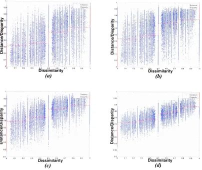
the goodness-of-fit is to examine a scatter

diagram,

also known as a Sheppard diagram. A scatter diagramis "aplot _comparing the

distances derived

by

[multidimensional scaling] and the transformed data

(disparities)

with the original data values or

proximities."

(Schiffman,

et _al.,

1981,

p. 17). What the

scatter diagramcan tell us is whether the stress value is _reliable, ifthere is

degeneracy,

One

thing

tolook for in a scatterdiagram ofametric solution is how clearlythe

points fitsome curve. Whenthepoints seemtofitsomefunctionotherthan the

function/

assumed inthemodel (suchas a linear

function),

then the stress value willbe magnified

due to an incorrect assumption about the

function/

_{This may} be an indication that the

dataneeds to bereanalyzed. For a non-metric _solution, one can_only checkto see ifthe

function is monotonic. Ifit is non-monotonic then _{it may be necessary}to

try

adifferent

starting position. The general shape of a smooth curve drawn through the points can

sometimes provide information about the

data,

such as artifacts due to a particulardata

collection method.

Lastly,

ifthe data points on a scatter diagram are _strongly clumped,

this is a good indication ofdegeneracy. "If

degeneracy

occurs, the clustering it springs

from should be noted and considered, but no other conclusions should be drawn. In

particular, theverysmall stress should notbetakenas

indicating

goodfit ina substantive

sense, since it is obtained

by

_violating two tacit assumptions: that the true _relationship

between distance and _proximity is smooth, and that points should _only lie in the same

positionifthe _{corresponding} objects function as virtuallyidentical." (Kruskal and

Wish,

3.1.2

Dimensionality

It is possible to estimate the _underlying

dimensionality

ofthe _{data. One way} to

approachthis istocomputethe stress(or sstress)valueforeachof several configurations

representing a range ofdimensions.

By

_examining a plot ofdimension versus stress, it

maybe possible to find some clues about dimensionality. As thenumber ofdimensions

increases,

the stress value shoulddecrease. _{In many}cases, there will be an elbowinthe

curve atthe dimension that represents the true dimensionality. Figure 3-1 illustratesthis

concept where the true

dimensionality

ofthe data isthree dimensions.

However,

not all

datawillproduce such a clearindicationofdimensionality. Whenthat

happens,

itmaybe

possibleto interpreta range of possible dimensionsorit maynotbepossible tointerpret

dimensionality

at all.

(A

12 14

Dimension

FIGURE 3-1: Example of Dimension vs. Stress plot _suggesting

3.1.3

Configuration

The _primary output of multidimensional scaling is a low-dimensional

configurationof points that _graphicallyrepresents similaritiesinthedata.

By

examining

the _{configuration,} it is possible to look for clues that

help

to interpret the _organizing

conceptsinherentinthe data. Althoughtheconfiguration will attempttoproducethebest

spatial representation ofthe

data,

the orientation ofthe configuration is arbitrary. Take

for example Figure 3-2which demonstrates the two-dimensionalconfiguration_resulting

from multidimensional _scaling of the distances between ten cities. It is clear that the

dimensions north/south and east/west are not in alignment with the axes. The

configuration is still correct becausethe distances between thepoints wouldremain the

same iftheplotwere rotated sothat thedimensions didalign withtheaxes (Kruskaland

Wish, 1978,

Ch. 2). It is also possible that the dimensions are not orthogonal to one

another and that there _{may be only} one

dimension,

or _potentially more than two

dimensionsthatare interpretableon aparticular2-dimensionalconfiguration.

A configuration can exhibit local structure as well as global structure.

By

selecting a cluster of points within the global configuration and _performing

multidimensional _scaling on just these _objects, the new configuration _may reveal

additional structure that was _previously obscured. This type of neighborhood

interpretationcanleadtofurtherunderstandingofthe_organizingconceptsand_underlying

o E Q -500 Seatle 1 r SanFrancisco LosAngeles Denver -Chicago -Houston Washington_DC# Atlanta NYC

1 i i

Miami

-500 0 500

Dimension 1_(Miles)

FIGURE 3-2: Example of a 2-dimensional multidimensional _scaling

configuration ofdistances between 10cities.Theorientationisarbitrary.

3.2 DUAL

SCALING

Dual scaling is often referred to as principal component analysis for categorical

data

(Maraun,

et _al., 2005). Principal component analysis operates

by

_maximizing the

varianceforaset ofvariables,or principle components,whichare linearcombinationsof

the original variables. The principal components are orthogonal to one another which

minimizes _redundancy of information. Dual scaling accomplishesthe same goal except

that it operates on categorical data to produce multidimensional

decomposition

of the

dataas explained

by

Nishisato&Nishisato

(1994,

p. 8):

Whentheoptimal solutiondoesnotexplainthe data inanexhaustive_way,

dual scalingdetermines asecondset of scores and weightsthat_maximally explains the portion ofdata unexplained

by

the first optimal solution. If

scores and_{weights, dual scaling looks forthe third optimal set of scores}

and weights that _maximally explains the portion of the data left

unexplained

by

the first two solutions. This process continues until the

originaldata can_{be perfectly}reproduced

by

the solutions obtained so

far,

that

is,

until the data are _exhaustively analyzed. This process is called

multidimensional

decomposition

ofdata.

This type of decomposition identifies the solution that provides the most

information

first,

followed

by

the solution that provides the next largest amount of

information,

and so on. Thisprocess makes itpossible to representthemostinformation

with the fewestnumber of solutions. Theusefulness ofthe solutions canbe determined

by

the amount of_variability ofthe original data thatis included in the solutions and

by

theresearcher's_abilitytointerpretthesolutions.

There are _many aspects ofdual scaling that differentiate it from other types of

analysis. Some ofthe

key

characteristics of_{dual scaling} are listed

by

Nishisato

(1994,

Ch.

2)

and are summarizedhere:

1)

Dual scalingprovides a simpler,oftenclearer, descriptionof

data,

thus_serving as atechnique toformauseful_summaryofotherwise complexdata.

2)

It derives anumeric

(quantitative)

description from non-numeric

(qualitative)

data...

3)

Ithandlesanalysisof a_varietyof so-calledcategoricaldata...

4)

It offers an exhaustive analysis of information in the

data,

often through multidimensional analysis...

5)

Itserves as atechnique fordiscriminantanalysisofcategoricaldata.

7)

It uses

individual

differences in judgment to explore the

data,

rather than

averaging them out as in most statistical analyses. Individual differencesare often more

interesting

thanaverageresponses.

8)

It can _quantify qualitative information so that traditional analysis

(e.g.,

analysisof_{variance) for}quantitativedata_maybecarried out.

Thereare numeroustechniques _{for analyzing}theresults ofdualscaling. One very

useful outcome is the _abilityto visualizehigh-dimensional _{data. Humans normally have}

difficulty

visualizing greaterthan threedimensions. _{Multidimensional scaling}provides a

way torepresenthigh-dimensional data in alow-dimensional configurationas described

in section 3.1.3.

However,

there is _ultimately a loss of information when _performing

dimensional reduction. Thedimensionsthatresultfrommultidimensional _scaling are not

orthogonal and therefore _may contain _redundancy of information. This is where dual

scaling can provide some insight where multidimensional _scaling cannot. Because the

solutions of_{dual scaling} are _orthogonal, each successive solution can be considered an

addeddimensionwithnew information. Although it isstill notpossible tocreate a

high-dimensional graphical representation ofthis

information,

it is still possible to evaluate

dimensionsgreaterthan three.

By

examining the objects at either end of a particular

dimension,

it ispossibleto

develop

an interpretation about certain characteristics ofthe objects which _may lead to

clues aboutthe nature ofthevariance contained inthatdimension. Inother_words, ifthe

objects at _opposing ends are _{significantly different in} some _way,

identifying

_{what that}

differenceiswill provide someinformationaboutthe_underlyingstructureinthedata. For

dual scalinganalysisofimage categorization. Theeightimages fromtheone extreme are

allhistoric

buildings.

Theeightimages fromtheopposite extreme are comprisedof

land,

water, and air vehicles. In other _words, several modes of transportation vehicles are

represented.

''. , ,

8

fcetiiiuli

WW

YkMn-\

:

-.

FIGURE 3-3: Exampleof_evaluatingthenature of variance inthe fourth

dimensionofadual scalinganalysis. Even without a spatial_{configuration,} it ispossibletointerpretcharacteristics ofthisdimension.

This example illustrates an important point about _performing this type of

relatedto each other nor do

they

have tobe opposites of oneanother (such as light and

dark). Transportation vehicles are not the opposite of historic buildings. These two

categories ofimages _simply providedthe greatest amount ofvariance forthis particular

dimension _usingthis particular dataset. When the

dimensionality

becomes high enough

that the amount of variance represented

by

thatdimension is very small, then itwill no

longerbepossibletoderivea reasonable interpretation fortheobjectsattheextremes.

"The chief aim of adual _scalinganalysis isnot statistical inferencebutrather the

description of the high-dimensional categorical data structures that often arise in

psychological research. The researcher who believes he or she has found an

interesting

relationship through the employment of _{dual scaling should,} as per sound scientific

practiceingeneral, attempttoreplicate the

finding

atalaterdate."

(Maraun,

et_al.,

2005)

In the current _study, this is accomplished through simultaneous analysis through

multidimensional_scalingandhierarchicalclusteranalysis.

A general description of dual scaling and some its uses have been presented.

Althoughathorough treatmentofthemathematicsof_{dual scaling}is beyondthe scope of

this paper, an excellent source forthemathematical details canbe found in Chapter 6of

Nishisato(1994).

3.3

HIERARCHICAL

CLUSTER

ANALYSIS

The basic objective of _any cluster analysis algorithm is to discover natural

groupings of the objects. Because it is not _generally possible to explore all object

need to examine _every cluster.

Many

_clustering algorithms will _group n objects into a

fixed number of k clusters which must be specified in advance. Hierarchical cluster

analysis does not have such a requirement and instead builds a tree-like structure, or

hierarchy,

which representsall values ofk. This is achieved

by

_usingone oftwo general

approaches agglomerative hierarchical methods or divisive hierarchical methods.

(Kaufmanand

Rousseeuw, 1990,

Ch. 5).

3.3.1

Agglomerative

Hierarchical Methods

Agglomerative hierarchical methods begin with computation of a _similarity

matrixbetweentheobjects. The _{initial clustering is}defined as a singleobject per cluster

sothat there are the same number of clusters as objects. _{Groups containing} objects with

the greatest similarities are mergedto form the first distance level ofthe

hierarchy

(the

initial grouping ofindividual objects is consideredthe zero distance level). Thisprocess

continues

iteratively

until all objects are merged into a single cluster (Johnson and

Wichern, 2002,

Ch. 12). Mostimplementationsofhierarchicalclusteranalysis,

including

theMatlab implementationusedinthis study,areagglomerativehierarchicalmethods.

3.3.2 Divisive Hierarchical Methods

Divisive hierarchicalmethods operate inreverseofagglomerativemethods.After

computinga

dissimilarity

matrixbetween_{the objects,} all objects aregroupedintoasingle

cluster. The initial cluster is then divided into two clusters such that the

dissimilarity

greatest _{distance from the objects in the}

second _group or are the most dissimilar. The

process of

dividing

groups into subgroups continues until each _group contains _only a

single object(Johnsonand

Wichern, 2002,

Ch. 12).

Most software

implementations

of hierarchical cluster analysis do not include

divisive methods due to the high computational overhead required. While an

i i j n(n-l) . . .

agglomerative method contains possible combinations to evaluate, a divisive

method will have

2""1 - 1

possible combinations. Note that the agglomerative methods

will grow _{quadratically} as n increases while the divisive methods will grow

exponentially. The number of possible combinations to evaluate for a divisive method

can _{quickly "exceed} the current estimate of the number of atoms in the universe"

(Kaufman and

Rousseeuw, 1990,

pp. 253-254).

Therefore,

few implementations of

divisivemethodsexist.

3.3.3 Linkage Methods

Fortheagglomerative hierarchical methods, the maindifference betweenthemis

the manner in which linkage distance is calculated. Linkage describes the process

by

which groups are merged. There are seven distance _measures, also called linkage

methods, implemented in Matlab single, complete, average, weighted, centroid,

median, and Ward's. Everitt

(1974,

Ch.

2)

provides a good description of how each

linkage method is calculated (except for weighted linkage which _{is described in the}

1)

SINGLE

-This _method, alsoknown as thenearest neighbormethod,uses

the smallest _{distance between}objects. For groups with morethanone

object, distance is definedasthedistance betweentheirclosestobjects.

2)

COMPLETE

-This method, alsoknownasthefur