Rochester Institute of Technology
RIT Scholar Works
Theses Thesis/Dissertation Collections
3-1-2009
Fast unsupervised multiresolution color image
segmentation using adaptive gradient thresholding
and progressive region growing
Sreenath Rao Vantaram
Follow this and additional works at:http://scholarworks.rit.edu/theses
This Thesis is brought to you for free and open access by the Thesis/Dissertation Collections at RIT Scholar Works. It has been accepted for inclusion in Theses by an authorized administrator of RIT Scholar Works. For more information, please [email protected].
Recommended Citation
FAST UNSUPERVISED MULTIRESOLUTION COLOR
IMAGE SEGMENTATION USING ADAPTIVE GRADEINT
THRESHOLDING AND PROGRESSIVE REGION
GROWING
by
Sreenath Rao Vantaram
A Thesis submitted in Partial Fulfillment of the
Requirements for the Degree of
M
ASTER OF
S
CIENCE
In
E
LECTRICAL
E
NGINEERING
Approved by:
Prof.
Thesis Advisor – Dr.Eli Saber
Prof.
Thesis Committee Member – Dr.Sohail A. Dianat
Prof.
Thesis Committee Member and
Head of the Department of Electrical Engineering – Dr.Vincent Amuso
Department of Electrical Engineering,
Kate Gleason College of Engineering,
ROCHESTER INSTITUTE OF TECHNOLOGY,
Rochester, New York
Thesis Author Permission Statement
Title of Thesis : Fast Unsupervised Multiresolution Color Image Segmentation using Adaptive Gradient Thresholding and Progressive Region Growing.
Name of Author : Sreenath Rao Vantaram Degree : Master of Science Program : Electrical Engineering
College : Kate Gleason College of Engineering
I understand that I must submit a print copy of my thesis or dissertation to the RIT Archives, per current RIT guidelines for the completion of my degree. I hereby grant to the Rochester Institute of Technology and its agents the non-exclusive license to archive and make accessible my thesis or dissertation in whole or in part in all forms of media in perpetuity. I retain all other ownership rights to the copyright of the thesis or dissertation. I also retain the right to use in future works (such as articles or books) all or part of this thesis or dissertation.
Print Reproduction Permission Granted:
I, __Sreenath Rao Vantaram __, hereby grant permission to the Rochester Institute Technology to reproduce my print thesis or dissertation in whole or in part. Any reproduction will not be for commercial use or profit.
Signature of Author: _____________________________________ Date: ____________
Inclusion in the RIT Digital Media Library Electronic Thesis & Dissertation (ETD) Archive
I, __Sreenath Rao Vantaram __, additionally grant to the Rochester Institute of Technology Digital Media Library (RIT DML) the non-exclusive license to archive and provide electronic access to my thesis or dissertation in whole or in part in all forms of media in perpetuity.
I understand that my work, in addition to its bibliographic record and abstract, will be available to the world-wide community of scholars and researchers through the RIT DML. I retain all other ownership rights to the copyright of the thesis or dissertation. I also retain the right to use in future works (such as articles or books) all or part of this thesis or dissertation. I am aware that the Rochester Institute of Technology does not require registration of copyright for ETDs.
I hereby certify that, if appropriate, I have obtained and attached written permission statements from the owners of each third party copyrighted matter to be included in my thesis or dissertation. I certify that the version I submitted is the same as that approved by my committee.
DEDICATION
This thesis dedicated to my family
To my father, Mr. Viswanath Rao Vantaram, for his unparalleled and unique ways of
motivating me from time to time
To my mother, Mrs. Dharmavani Rao Vantaram, for her never-ending love
ACKNOWLEDGMENTS
I feel it to be a unique privilege combined with immense happiness to acknowledge
the contributions and support of all the wonderful people who have been responsible for
the completion of my master’s degree. The two years of graduate study at RIT has taught
me that creative instinct, excellent fellowship and perceptiveness are the very essence of
engineering. It not only imparts knowledge but also lays emphasis on the overall
development of an individual. I am extremely appreciative of RIT, especially Department
of Electrical Engineering in this regard.
I would like to thank Dr. Sohail Dianat, Dr. Vincent Amuso and Dr. Eric Peskin for
their valuable assistance that has made this work possible. Also, I extend my sincerest
gratitude to all my friends/colleagues in and outside the ‘signal processing community’ at
RIT for their encouragement and being a part of a grueling yet enjoyable educational
experience. I am grateful to Mr. Mark Shaw, Mr. Ranjit Bhaskar and the Hewlett Packard
Company for their generosity in supporting and sponsoring this research and showing
tremendous confidence and satisfaction in my work and the results achieved.
Finally, I am extremely indebted to the man whose unique ways of teaching and
relentless guidance is solely responsible for transmuting an ordinary student like me to a
confident graduate researcher. His inspired notion that “if intellect can find the right
question, learning and research help find the answer, seek and thou shall find”, has been
instrumental in what I am today. Thank you Dr Eli Saber for everything that you have
ABSTRACT
In this thesis, we propose a fast unsupervised multiresolution color image segmentation
algorithm which takes advantage of gradient information in an adaptive and progressive
framework. This gradient-based segmentation method is initialized by a vector gradient
calculation on the full resolution input image in the CIE L*a*b* color space. The
resultant edge map is used to adaptively generate thresholds for classifying regions of
varying gradient densities at different levels of the input image pyramid, obtained
through a dyadic wavelet decomposition scheme. At each level, the classification
obtained by a progressively thresholded growth procedure is combined with an
entropy-based texture model in a statistical merging procedure to obtain an interim segmentation.
Utilizing an association of a gradient quantized confidence map and non-linear spatial
filtering techniques, regions of high confidence are passed from one level to another until
the full resolution segmentation is achieved. Evaluation of our results on several hundred
images using the Normalized Probabilistic Rand (NPR) Index shows that our algorithm
outperforms state-of the art segmentation techniques and is much more computationally
TABLE OF CONTENTS
Thesis Author Permission Statement ... II
Dedication ... III
Acknowledgments ... IV
Abstract ... V
Table of Contents ... VI
List of Figures ... VIII
List of Tables ... XVII
Chapter 1: INTRODUCTION ...1
1.1 Objectives and Motivations ...1
1.2 Literature Review ...1
1.3 Contributions...6
1.4 Potential Applications ...8
1.5 Thesis Outline ...11
Chapter 2: BACKGROUND ...12
2.1 Wavelet Transform ...12
2.2 Multiresultion Image Decomposition/Representation ...14
2.3 CIE L*a*b* Color Space ...19
Chapter 3: Proposed Algorithm ...21
3.1 Adaptive Gradient Thresholding...23
3.2 Dyadic Wavelet Decomposition ...32
3.5 Texture Characterization and Region Merging ...61
Chapter 4: Evaluation of Segmentation Algorithms ...65
4.1 Rand Index ...66
4.2 Probabilistic Rand (PR) Index ...67
4.3 Normalized Probabilistic Rand (NPR) Index ...68
Chapter 5: Results and Discussions...71
Chapter 6: Conclusions and Future Work ...85
LIST OF FIGURES
Figure 1: Overview of proposed approach ...6
Figure 2: Image Rendering utilizing MAPGSEG ...9
Figure 3: CBIR utilizing MAPGSEG ...10
Figure 4 a): Multiresolution image representation ...18
Figure 4 b): Analysis filter bank ...18
Figure 5: Block diagram of MAPGSEG ...22
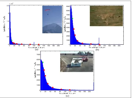
Figure 6 a): Gradient histogram of ‘Parachute’ image ...23
Figure 6 b): Gradient histogram of ‘Cheetah’ image ...23
Figure 6 c): Gradient histogram of ‘Cars’ image ...23
Figure 7 a): Gradient histogram RGB Vs. CIEL*a*b* of ‘Parachute’ image ...26
Figure 7 b): Gradient histogram RGB Vs. CIEL*a*b* of ‘Cheetah’ image ...26
Figure 7 c): Gradient histogram RGB Vs. CIEL*a*b* of ‘Cars’ image ...26
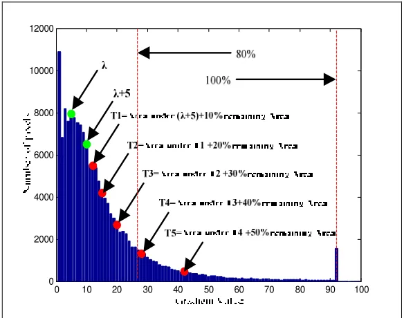
Figure 8: Histogram based adaptive gradient thresholding ...28
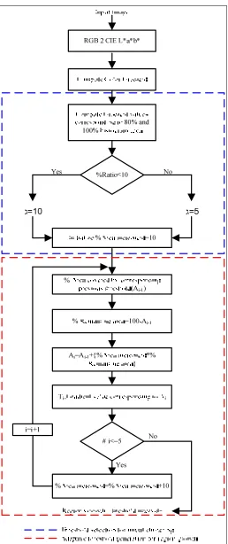
Figure 9: Flowchart of adaptive gradient thresholding ...30
Figure 10 a): Static Vs Adaptive thresholds ...31
Figure 10 b): Multiresolution gradient histograms ...31
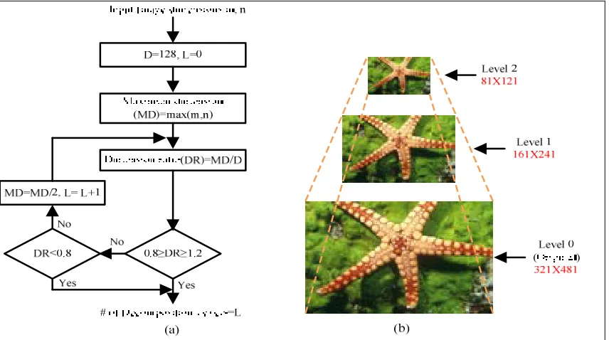
Figure 11 a): Determination of number of decomposition levels ...33
Figure 11 b): Two level decomposition with corresponding designations ...33
Figure 12: Progressive region growth involving distributed dynamic seed addition.35 Figure 13 a): Cars-L*a*b* (81 X121) ...36
Figure 13 d): Logical seed map ...36
Figure 13 e): Logical seed map after dilation ...36
Figure 13 f): Padded seeds in the gradient map ...36
Figure 13 g): Initial clusters at λ+5 (10), 25*MSS...36
Figure 13 h): Parent seeds ...36
Figure 14 a): Logical PS map ...37
Figure 14 b): Unassigned pixels ...37
Figure 14 c): Large unassigned regions ...37
Figure 14 d): Small and isolated unassigned pixel locations ...37
Figure 14 e): Small and isolated unassigned pixel map after dilation ...37
Figure 14 f): Small and isolated unassigned pixel borders ...37
Figure 14 g): Small and isolated unassigned pixel neighborhood labels ...37
Figure 14 h): Small and isolated unassigned pixel label assignment ...37
Figure 15 a): Parent seeds map after seed saturation ...40
Figure 15 b): New seeds after threshold increment ...40
Figure 15 c): Parent seed borders...40
Figure 15 d): Adjacent child seeds map ...40
Figure 15 e): Seed map after one interval of the region growth procedure ...40
Figure 15 f): Seeds obtained during the first stage of dynamic seed addition procedure ...40
Figure 15 g): Parent seeds for the next region growth interval ...40
Figure 16 a): Cars-L*a*b*(161X241) ...43
Figure 16 c): Interim segmentation (81X121) ...43
Figure 16 d): High confidence seeds (161X241) ...43
Figure 16 e): Padded high confidence seeds in the gradient map...43
Figure 17 a): Gradient histogram comparison of ‘Cars’ image Vs unsegmented pixels, at the CDS (161X241): Entire histogram ...45
Figure 17 b): Gradient histogram comparison of ‘Cars’ image Vs unsegmented pixels, at the CDS (161X241): Zoomed view 1 ...45
Figure 17 c): Gradient histogram comparison of ‘Cars’ image Vs unsegmented pixels, at the CDS (161X241): Zoomed view 2 ...45
Figure 18 a): Classifying threshold intervals for DDSA...46
Figure 18 b): Zero crossing curve between red and green curves in (a) ...46
Figure 19 a): At decision boundary 1 (gradient value 22): Agglomeration of seeds obtained ...49
Figure 19 b): At decision boundary 1 (gradient value 22): Overall seed map prior to region growth ...49
Figure 19 c): At exact point of intersection (gradient value 108): (c) Agglomeration of seeds obtained ...49
Figure 19 d): At exact point of intersection (gradient value 108): (c) Overall seed map prior to region growth ...49
Figure 20 a): Cars-L*a*b* (321X481) ...50
Figure 20 b): Corresponding color gradient ...50
Figure 20 c): Interim segmentation (161X241) ...50
Figure 20 e): Padded high confidence seeds in the gradient map...50
Figure 20 f): Agglomeration of seeds obtained at various thresholds lower than the decision gradient value ...50
Figure 21: Gradient histogram comparison of ‘Cars’ image Vs unsegmented pixels, at the CDS (321X481) ...51
Figure 22 a): MAPGSEG region growth map: Level1 ...52
Figure 22 b): MAPGSEG region growth map: Level0 ...52
Figure 22 c): Neighborhood label assignment: Level1 ...52
Figure 22 d): Neighborhood label assignment: Level0 ...52
Figure 22 e): Iterative morphological label assignment: Level1 ...52
Figure 22 f): Iterative morphological label assignment: Level0 ...52
Figure 22 g): V2.2 region growth map: before residual pixel label assignment ...52
Figure 22 h): V2.2 region growth map: after residual pixel label assignment ...52
Figure 23: Seed transfer module ...54
Figure 24 a): Interim output: Level2 ...54
Figure 24 b): Interim output: Level1 ...54
Figure 24 c): Zero insertion yielding: Level1 ...54
Figure 24 d): Zero insertion yielding: Level0 ...54
Figure 24 e): Neighborhood label assignment: Level1 ...54
Figure 24 f): Neighborhood label assignment: Level0 ...54
Figure 25: Quantized gradient map at level1 (161X241) ...57
Figure 26 b): High confidence pixel locations corresponding to quantization levels 5
and 12 at a level1: Color map ...57
Figure 26 c): High confidence pixel locations corresponding to quantization levels 5 and 12 at a level1: Zoomed in version of circular area in (b) ...57
Figure 27 a): High confidence pixel locations color map ...60
Figure 27 b): MSBR ...60
Figure 27 c): High confidence pixel locations color map after MSBR removal ...60
Figure 27 d): Large confident regions ...60
Figure 27 e): Large confident regions seed borders ...60
Figure 27 f): MSBR labels ...60
Figure 27 g): High Confidence MSBR regions ...60
Figure 27 h): A-priori information after border refinement ...60
Figure 28: Euclidean space representation of L*a*b* ...63
Figure 29 a): Multiresolution representation of: original RGB ‘Star Fish’ image ....72
Figure 29 b): Multiresolution representation of: Color converted ‘Star Fish’ image72 Figure 29 c): Multiresolution representation of: Color gradient ...72
Figure 29 d): Multiresolution representation of: Seeds maps at the end of progressive region growth ...72
Figure 29 e): Multiresolution representation of: Entropy based texture maps ...72
Figure 29 f): Multiresolution representation of: Interim and final segmentation outputs ...72
Figure 30 a): Interim Segmentation at: Level2 ...73
Figure 30 c): A-priori information at level1 ...73
Figure 30 d): Interim Segmentation at: Level1 ...73
Figure 30 e): Interim Segmentation at: Upconverted to Level0 ...73
Figure 30 f): A-priori information at level0 ...73
Figure 30 g): MAPGSEG final segmentation output ...73
Figure 31 a): Church Results: Original ...75
Figure 31 b): Church Results: GRF ...75
Figure 31 c): Church Results: JSEG ...75
Figure 31 d): Church Results: DCGT ...75
Figure 31 e): Church Results: GSEG-V2.2...75
Figure 31 f): Church Results: MAPGSEG ...75
Figure 32 a): Parachute Results: Original ...75
Figure 32 b): Parachute Results: GRF...75
Figure 32 c): Parachute Results: JSEG ...75
Figure 32 d): Parachute Results: DCGT ...75
Figure 32 e): Parachute Results: GSEG-V2.2 ...75
Figure 32 f): Parachute Results: MAPGSEG ...75
Figure 33 a): Cheetah Results: Original ...76
Figure 33 b): Cheetah Results: GRF ...76
Figure 33 c): Cheetah Results: JSEG ...76
Figure 33 d): Cheetah Results: DCGT ...76
Figure 33 e): Cheetah Results: GSEG-V2.2 ...76
Figure 34 a): Nature Results: Original ...77
Figure 34 b): Nature Results: GRF ...77
Figure 34 c): Nature Results: JSEG ...77
Figure 34 d): Nature Results: DCGT ...77
Figure 34 e): Nature Results: GSEG-V2.2 ...77
Figure 34 f): Nature Results: MAPGSEG ...77
Figure 35 a): Cars Results: Original ...77
Figure 35 b): Cars Results: GRF ...77
Figure 35 c): Cars Results: JSEG ...77
Figure 35 d): Cars Results: DCGT ...77
Figure 35 e): Cars Results: GSEG-V2.2 ...77
Figure 35 f): Cars Results: MAPGSEG ...77
Figure 36 a): Island Results: Original ...78
Figure 36 b): Island Results: GRF ...78
Figure 36 c): Island Results: JSEG ...78
Figure 36 d): Island Results: DCGT ...78
Figure 36 e): Island Results: GSEG-V2.2 ...78
Figure 36 f): Island Results: MAPGSEG ...78
Figure 37: Human segmentations for the ‘Island’ image provided by University of California, at Berkeley...78
Figure 38 a): Asians Results: Original ...79
Figure 38 b): Asians Results: GRF ...79
Figure 38 d): Asians Results: MAPGSEG Level2 ...79
Figure 38 e): Asians Results: MAPGSEG Level1 ...79
Figure 38 f): Asians Results: MAPGSEG Level0...79
Figure 39: Human segmentations for the ‘Asians’ image provided by University of California, at Berkeley...79
Figure 40 a): Tree Results: Original ...80
Figure 40 b): Tree Results: GRF ...80
Figure 40 c): Tree Results: JSEG ...80
Figure 40 d): Tree Results: MAPGSEG Level2 ...80
Figure 40 e): Tree Results: MAPGSEG Level1 ...80
Figure 40 f): Tree Results: MAPGSEG Level0 ...80
Figure 41 a): Road Results: Original ...80
Figure 41 b): Road Results: GRF ...80
Figure 41 c): Road Results: JSEG ...80
Figure 41 d): Road Results: MAPGSEG Level2 ...80
Figure 41 e): Road Results: MAPGSEG Level1 ...80
Figure 41 f): Road Results: MAPGSEG Level0 ...80
Figure 42 a): NPR scores distribution for 300 images of the Berkeley database: GRF. ...80
Figure 42 b): NPR scores distribution for 300 images of the Berkeley database: JSEG...80
Figure 42 d): scores distribution for 300 images of the Berkeley database: GSEG ..81
Figure 42 e): NPR scores distribution for 300 images of the Berkeley database: MAPGSEG ...81
Figure 42 f): NPR scores distribution for 300 images of the Berkeley database: All algorithms distributions superimposed...81
Figure 43 a): Computational time comparison utilizing Berkeley database (321X421): MAPGSEG, GSEG and DCGT ...83
Figure 43 b): Computational time comparison utilizing Berkeley database (321X421): Various levels of MAPGSEG ...83
Figure 43 c): Computational time comparison utilizing large resolution image database (750X1200): MAPGSEG, GSEG ...83
Figure 43 d): Computational time comparison utilizing large resolution image database (750X1200): Various levels of MAPGSEG ...83
Figure 44 a): Segmentation results: Original ...84
Figure 44 b): Segmentation results: GSEG ...84
LIST OF TABLES
Table 1: Daubechies 9/7 analysis filter coefficients ...19
Table 2: MAPGSEG threshold selection for a two level decomposition (‘Cars’
image) ...51
Table 3: Evaluation of MAPGSEG using 300 images of the Berkeley database in
comparison to published work ...82
Table 4: Evaluation of various levels of MAPGSEG using 300 images of the
Berkeley database ...82
Table 5: Evaluation of various levels of MAPGSEG using 445 large resolution
Chapter 1: INTRODUCTION
1.1
OBJECTIVES AND MOTIVATIONSUnsupervised image segmentation is a long standing problem in many computer
vision and image understanding applications. Segmentation is defined as the meaningful
partitioning of images into non-overlapping homogenous regions exhibiting similar
features or image content. It finds a place in many important applications such as image
rendering/indexing, object classification, content based image retrieval, medical imaging,
image/video compression, image/video surveillance and multi-media applications. Few
segmentation algorithms have been developed that efficiently facilitate: 1) selective
access and manipulation of individual content in images based on desired level of detail,
2) handling sub sampled versions of the input images and decently robust to scalability,
3) a good compromise between quality and speed, laying the foundation for fast and
intelligent object/region based real-world applications of color imagery.
1.2 LITERATURE REVIEW
Many grayscale/color domain methodologies have been adopted in the past to tackle
this ill-defined problem (see [1, 2] for comprehensive surveys). Initial multiscale research
was aimed to overcome drawbacks being faced by Bayesian approaches for
segmentation/classification, using Markov Random Fields (MRF’s) and Gibbs Random
Field’s (GRF’s) estimation techniques. Derin et al. [3] proposed a method of segmenting
clustering algorithm using adaptive and spatial constraints, and the Gibbs Random Field
(GRF) model to achieve segmentation in the gray scale domain. Chang et al. [5] extended
this to color images by assuming conditional independence of each color channel.
Improved segmentation and edge linking was achieved by Saber et al. [6] who combined
spatial edge information and the regions resulting from a GRF model of the segmentation
field. Bouman et al. [7] proposed an algorithm for segmenting textured images consisting
of regions with varied statistical profiles using a causal Gaussian autoregressive model
and a MRF representing the classification of each pixel at various scales. However most
of the aforementioned methods suffered from the fact that the obtained estimates could
not be calculated exactly and were computationally prohibitive. To overcome these
problems, Bouman et al. [8] extended his work by incorporating a multiscale random
field model (MSRF) and a sequential MAP (SMAP) estimator. The MSRF model was
used to capture the characteristics of image behavior at various scales. However, the
work in [7,8] had either used single scale versions of the input image, or multiscale
versions of the image with the underlying hypothesis that the random variables at a given
level of the image data pyramid were independent from the ones at other levels.
Comer et al. [9] used a multiresolution Gaussian autoregressive model (MGAR) for a
pyramid representation of the input image and “maximization of posterior marginals”
(MPM) for pixel label estimates. He established correlations for these estimates at
different levels using the interim segmentations corresponding to each level. He extended
his work in [10] by using a multiresolution MPM model for class estimates and a
multiscale MRF to establish interlevel correlations into the class pyramid model. Liu et
segmentation of the input image using MRF’s in a quad-tree structure. An MRF model in
combination with the discrete wavelet transform was proposed by Tab et al. [12] for
effective segmentations with spatial scalability, producing similar patterns at different
resolutions. Cheng et al. [13] incorporated Hidden Markov Models (HMM’s) for
developing complex contextual structure, capturing textural information, and correlating
among image features at different scales unlike previously mentioned MRF models. The
methods usefulness was illustrated on the problem of document segmentation where intra
scale contextual dependencies can be imperative. A similar principle was applied by Won
et al. [14] who combined HMM and Hidden Markov Tree (HMT) forming a hybrid
HMM-HMT model to establish local and global correlations for efficient block-based
segmentations.
Watershed and wavelet-driven segmentation methods has been of interest for many
researchers. Vanhamel et al. [15] proposed a scheme constituting a non-linear anisotropic
scale space and vector value gradient watersheds in a hierarchical frame work for
multiresolution analysis. In a similar framework Makrogiannis et al. [16] proposed
watershed based segmentations utilizing a fuzzy dissimilarity measure and connectivity
graphs for region merging. Jung et al. [17] combined orthogonal wavelet decomposition
with the watershed transform for multiscale image segmentation.
Edge, contour and region structure are other features that have been adopted in
various approaches for effective segmentations. Tabb et al. [18] instituted a multiscale
approach where the concept of scale represented image structures at different resolutions
rather than the image itself. The work involved performing a Gestalt analysis facilitating
other hand, Gui et al. [19] obtained multiscale representations of the image using
weighted TV flow and used active contours for segmentation. The contours at one level
were given as input to the next higher level to refine the segmentation outcome at that
level. Munoz et al. [20] applied fusion of region and boundary information, where the
later was used for initializing a set of active regions which in turn would compete for
pixels in the image in manner that would eventually minimize a region-boundary based
energy function. Sumengen et al. [21] showed through his work that multiscale
approaches are very effective for edge detection and segmentation of natural images.
Mean shift clustering followed by a minimum description length (MDL) criterion was
used by Luoet al. [22] for the same purpose.
Fusion of color and texture information is an eminent methodology in multiresolution
image understanding/analysis research. Deng et al. [23] proposed a method prominently
known as JSEG that performed color quantization and spatial segmentation in
combination of a multiscale growth procedure for segmenting color-texture regions in
images and video. Pappas et al. [24] utilized spatially adaptive features pertaining to
color and texture in a multiresolution structure to develop perceptually tuned
segmentations, validated using photographic targets. Dominant color and homogenous
texture features (HTF) integrated with an adaptive region merging technique were
employed by Wan et al. [25] to achieve multiscale color-texture segmentations.
The task of segmenting images in perceptually uniform color spaces is an ongoing
area of research in image processing. Paschos et al. [26] proposed an evaluation
methodology for analyzing the performance of various color spaces for color texture
uniform/approximately uniform color spaces such as L*a*b*, L*u*v* and HSV possess a
performance advantage over RGB, a non uniform color space traditionally used for color
representation. The use of these color spaces was found to be suited for the calculation of
color difference using the Euclidean distance, employed in many segmentation
algorithms. Yoon et al. [27] utilized this principle to propose a Color Complexity
Measure (CCM) for generalizing the K-means clustering algorithm, in the CIE L*a*b*
space. Chen et al. [28] employed color difference in the CIE L*a*b* space to propose
directional color contrast segmentations. Contrast generation as a function of the
minimum and maximum value of the euclidean distance in the CIE L*a*b* space, was
seen in the work of Chang et al. [29]. This contrast map, subjected to noise removal and
edge enhancement to generate an Improved Contrast Map (ICMap), was the proposed
solution to the problem of over-segmentation in the JSEG algorithm. More recently, Gao
et al. [30] introduced a ‘narrow-band’ scheme for multiresolution processing of images
by utilizing the MRF expectations-maximization principle in the L*u*v* space. This
technique was found to be competent especially for segmenting dermatoscopic images.
Lefevre et al. [31] performed multiresolution image segmentation in the HSV space,
applied to the problem of background extraction in outdoor images.
Color gradient-based segmentation is a new contemporary methodology in the
segmentation realm. Dynamic color gradient thresholding (DCGT) was first seen in the
work by Balasubramanian et al. [32]. The DCGT technique was primarily used to guide
the region growth procedure, laying emphasis on color homogenous and color transition
regions without generating edges. However this algorithm faced problems of over
expensive. Ugarriza et al. [33] proposed a Gradient SEGmentation (GSEG) algorithm
that was an enhanced version of the DCGT technique, by incorporating an entropic
texture descriptor and a multiresolution merging procedure. The method brought
significant improvement in the segmentation quality and computational costs, but was not
fast enough to meet real time practical applications.
1.3CONTRIBUTIONS
In this thesis we propose a new unsupervised Multiresolution Adaptive and
Progressive Gradient SEGmentation (MAPGSEG) algorithm, facilitating: 1) robust
handling of sub-sampled versions of the original input image, 2) multiple segmentation
outputs representing distinct levels of detail, desired by the user, 3) a potential solution
that computationally measures up to the demands of most practical applications involving
segmentation, 4) an effective compromise between quality and speed.
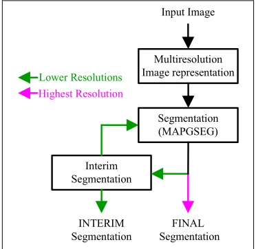
Input Image
Multiresolution Image representation
Segmentation (MAPGSEG)
FINAL Segmentation Interim
Segmentation
INTERIM Segmentation
Lower Resolutions Highest Resolution
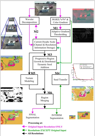
[image:24.612.231.417.463.644.2]An overview of the proposed approach is shown in Fig. 1. The algorithm begins with
a vector gradient computation [34] in CIE L*a*b* color space on the input image at full
resolution, followed by a wavelet decomposition to obtain a pyramid representation of it.
Starting at the smallest resolution, the functionality of the CIE L*a*b* space includes,
but is not limited to, automatically and adaptively generating thresholds required for
initial clustering, as well as carrying out a computationally efficient region growth
procedure. The resultant classification is combined with an entropy-based texture model
and statistical procedure to obtain an interim segmentation representing a certain degree
of detail, in comparison to the original input. The up scaled version of this segmentation
map is utilized as the a-priori knowledge for segmenting the next higher resolution.
Furthermore, this up scaled segmentation is put through confidence computation utilizing
the gradient map of the current resolution and non-linear spatial filtering techniques.
Regions of high confidence are passed to a fresh run of the algorithm, at the current
resolution, subjecting it to lesser work in comparison to its previous stage. However, the
thresholds for region growth and distributed dynamic seed generation at higher
resolutions are selected in a progressive manner based on a histogram analysis of the
gradient values of the image at the current resolution and the unsegmented ‘low
confidence’ regions. The aforementioned procedure takes into account the fact that low
gradient regions in images can be segmented at relatively small resolutions in comparison
to the size of the original, and to this effect, only when more detail is required do we need
to perform segmentation at subsequent bigger resolutions. Our algorithm is entirely
implemented in MATLAB and tested on a large database of ~745 images. Its
NPR index on the same test bed of images in Berkeley database [42] comprising of 300
images (inclusive in the testing database). Furthermore, a comprehensive runtime
evaluation was performed on all 745 images with varied resolutions (from 321X481 to
768X1024), and the two evaluations combined show that the MAPGSEG is significantly
less computationally intensive, maintaining benchmark segmentation quality with the
capabilities of facilitating real time performance.
1.4POTENTIAL APPLICATIONS
Image segmentation has wide spread medical, military and commercial interests. Our
algorithm is designed from a commercial standpoint with an enormous emphasis on
performance. Here we illustrate few applications that can take advantage of the
capabilities our algorithm.
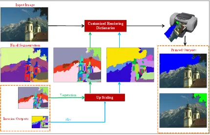
1.4.1 IMAGE RENDERING
Rendering is often utilized in cameras and printers to acquire images with superior
visual or print quality. This application is a tool that comes closest to transmuting reality
to a photograph or printer output. A typical region/object oriented rendering algorithm,
designed for better print quality is shown in Fig. 2. The rendering procedure illustrated is
commenced by segmenting the input image using the MAPGSEG algorithm. As can be
seen, the output of the MAPGSEG consists of multiple interim results and one final
segmentation. Interim output1 obtained at the lowest resolution, represents a coarse
segmentation where only the low gradient regions such as the sky and mountain are well
we see more detail associated with vegetation and manmade structures. The final result
shows fine detail with well defined edges for all regions. This hierarchy of detail and
corresponding computational performance can be utilized for efficient and intelligent
rendering.
Fig.2 Image rendering utilizing MAPGSEG
If the rendering objective is just limited to the low gradient regions then customized
rendering intents are applied to these regions extracted from the up scaled coarse
segmentation, to achieve better print quality. The advantage is that the coarse result
achieved is much faster than its higher resolution counterparts. Furthermore, the up
scaling operation is performed to acquire a coarse segmentation at the same resolution of
the input image. As the scope of the rendering intentions are increased, higher resolution
[image:27.612.109.539.181.458.2]segmentation-integrated rendering approach is much more flexible and computationally
inexpensive than utilizing an approach that operates only on a single scale.
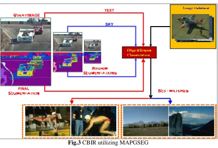
1.4.2 CONTENT BASED IMAGE RETRIEVAL (CBIR)
Content based image retrieval also known as Query By Image Content (QBIC) is
defined as the process of sifting through large archives of digital images based on color,
texture, orientation features, and other image content such as objects and shapes.
Fig.3 CBIR utilizing MAPGSEG
Fig. 3 illustrates the advantage of incorporating the MAPGSEG algorithm for
region-based image retrieval. Here again, if the objective of the retrieval procedure is to acquire
images with low gradient regions such as sky then a lower resolution of the input query
image would suffice. The query image at the lower resolution and its corresponding
[image:28.612.109.542.263.558.2]sky without much hindrance, owed to its low gradient content. Moreover, the
aforementioned inputs along with the classification output can be used for an effective
retrieval procedure. The computational costs are significantly reduced because all
operations are performed at a lower resolution of the query image. Regions of higher
gradient densities (such as text in Fig. 3) can be similarly used for retrieval at bigger
resolutions.
1.5 THESIS OUTLINE
The remainder of this report is organized as follows. In Chapter2, a review of the
necessary background required to effectively implement our algorithm is presented. The
proposed algorithm, presented in Chapter3, is subdivided into five Sections: 3.1
introduces the adaptive gradient thresholding module, 3.2 explains the dyadic wavelet
decomposition scheme, 3.3 illustrates the multiresolution region growth and distributed
dynamic seed addition procedure, and Sections 3.4 and 3.5 recap the texture modeling
and statistical merging procedure used in the GSEG (V2.2) algorithm. The NPR
technique used for evaluating various segmentation results is discussed in Chapter4.
Results obtained in comparison to popular segmentation methods and human
Chapter 2: BACKGROUND
This section familiarizes some technical concepts that are required for the optimal
implementation and understanding of our algorithm. Firstly, we provide a mathematical
insight into the Wavelet Transform, the foundation on which the wavelet theory has been
established. Secondly we provide a brief discussion involving the extension of the
wavelet transform for pyramidal image representations and its practical implementation
using filter banks, imperative from a multiresolution analysis standpoint. Thirdly, we give
a brief description of the CIE L*a*b* color space and its characteristics that helped us
develop this efficient algorithm.
2.1 WAVELET TRANSFORM
Wavelets are powerful tools capable of dividing data into various frequency bands
describing, in general, the horizontal, vertical, and diagonal spatial frequency
characteristics of the data. A detailed mathematical analysis of initial multiresolution
image representation models and its relation to the Wavelet Transform (WT) can be seen
in the work of Mallat et al. [35]. Let L2(R)denote the Hilbert space of square integrable
1-D functionsf(x). The dilation of this function by a scaling component scan be
represented as:
) ( )
(x sf sx
fs = (1)
translation and dilation of a function ψ(x). Here, ψ(x)is called a wavelet and the class of
functions is defined, using (1), by 2
) , ( ))) ( ( ( R u s u x s
sψ − ∈ . To this effect, the WT is defined
as: dx u x s s x f u s
Wf =∫+∞ −
∞
− ( ) ( ( ))
) ,
( ψ (2)
An inner product representation of Eq. (2) can be written as:
) ( ), ( ) ,
(s u f x x u
Wf = ψs − (3)
To enable the reconstruction of f(x)from Wf (s,u)the Fourier transform of ψˆ(x)must comply with:
∫
+∞ +∞ < = 0 2 | ) ( ˆ | ω ω ω ψ ψ dC (4)
Eq. (4) signifies that ψˆ(0)=0,and ψˆ(x)is small in the vicinity of ω =0. Therefore, ψ(x)
can be construed as the impulse response of a Band Pass Filter (BPF). WT can be now
written as a convolution product given as:
) ( ~ * ) ,
(s u f u
Wf = ψs (5)
where ψ~s(x)=ψs(−x). Thus, a WT can be interpreted as a filtering of f(x)with a BPF
whose impulse response is ψ~s(x). Furthermore from the aforementioned discussion we
see that the resolution of a WT varies with scale parameter s. Sampling s, u and
selecting a sequence of scales j j Z ∈
)
(α , can be utilized to discretize the WT. Thus Eq. (5)
2.2 MULTIRESOLUTION IMAGE DECOMPOSITION/REPRESENTATION
A signal f(x) at resolution r can be acquired by filtering f(x)with a Low Pass Filter
(LPF) whose bandwidth is proportional to the desired uniform sampling rate r, of the
filtered result [35]. To negate the possibility of inconsistency with resolution variation
these LPF’s are obtained from a function θ(x)dilated by the resolution parameter r and
can be represented in form identical to that of Eq. (1), given below:
) (rx r
r θ
θ = (8)
Likewise to Eq. (7) the discrete approximation of a function f(x)on a dyadic array of
resolutions j j Z ∈
) 2
( can be represented as:
(
)
(
f jn)
n Zf
A j j
∈ −
= * 2
2
2 θ (9)
Eq. (9) represents an important category of the DWT known as orthogonal wavelets.
Consequently, a wavelet orthonormal basis corresponds to the DWT for α =2andβ =1.
Although orthonormal basis can be constructed for scale sequences other than j j Z ∈
) 2
( , in
general dyadic scales are used because they result in simple decomposition algorithms.
For pyramidal multiresolution image representations, θ(x)is chosen with a Fourier
transform defined by:
(
)
∏ = +∞ = − − 1 2 ) ( ˆ p p i e U ω ωθ (10)
where
(
iω)
e
Subsequently, the approximation of a function f(x)at a scale j j Z ∈
) 2
( is obtained by
filtering A2j+1fn∈Zwith Uand restoring every alternate sample in the resultant convolution,
written as: Z n n U f
A j = ∈
=
Λ 2+1 * (λ ) (11)
Z n n
f
A2j =(λ2 ) ∈ (12)
where
(
(
)
)
Z n j n f f
A j j
∈ + − + + = ) 1 ( 2
2 1 *θ 1 2 . Eq. (11) and (12) can be utilized iteratively to find the
approximation of the signal f(x) at any dyadic resolution (2− , >0
J
J where
J j≥− ≥
0 ).
Furthermore the apart from an estimate, the details of a signal at a particular resolution
can be also obtained. From Eq. (11) and (12) we see that A j1f
2+ has double the number of
samples inA jf
2 . Thus the details D2j f at a resolution j
2 is given by:
f A f A f D e j j j 2 2
2 = +1 − (13)
where Ae f j
2 is the expanded version of A jf
2 acquired by inserting a zero between each of
its samples followed by filtering the resultant signal with an LPF.
Altogether, the previously mentioned discussion can be utilized to develop a
multiresolution wavelet model. Earlier, Eq. (9) represented the estimate of f(x) at a scale
of 2j, utilizing Eq. (3) and (5) this estimate can be re-written as:
(
)
(
j)
n Zn x x f f
A j j
∈ − −
= ( ),~ 2
2
2 θ (14)
orthogonal projection of the signal on the array of all possible estimates designated by a
vector space V j
2 , a proposition of the projection theorem. The array
( )
V2j j∈Zis known asthe multiresolution approximation of L2(R), requires an orthonormal basis for its
computation. An orthonormal basis can be acquired by dilating and translating a scaling
functionφ(x), denoted at any 2j resolution (from Eq. (1) or (8)) as
) 2 ( 2 ) (
2 x x
j j
j φ
φ = .
Thus from the initial definition of the WT the class of functions
(
)
Z n j n x j ∈ −
−2 )
(
2
φ can be
called the orthonormal basis of the vector space V j
2 . From Eq. (10) we have:
(
)
∏ = +∞ = − − 1 2 ) ( ˆ p p i e H ω ωφ (15)
Here H
(
e−iω)
is the transfer function of a discrete filter. Furthermore if:(
−iω)
2 +(
− −iω)
2 =1e H e
H (16)
Then the discrete filters represented by H =
( )
hn n∈Z are called as quadrature mirror filters.In addition, the orthogonal projection of f(x) on V j
2 is given by:
(
u n)
(
x n)
u f x f P j Z n j
V j j
j
− ∈
− −
∑ −
= ( ), 2 2
) )( ( 2 2 2 φ
φ (17)
represents the best estimate of f(x). We now express A j f
2 in terms of ( )
~
x
φ instead of
) (x
θ , φ(x)being an LPF. Thus Eq. (9) becomes:
Utilizing Eq. (15), (18) in conjunction with Eq. (11) and (12) the discrete approximations
f A j
2 of a signal f(x)at a resolution j
2 can be obtained. In addition, the approximation of
a signal at a resolution 1
2j+ in V2j+1can be considered to be better than it counterpart at a
resolution j
2 in V j
2 . The difference in detail between the two resolutions is given by the
orthogonal projection of f(x) on the orthogonal complement of 1
2j+
V in V j
2 , denoted as
j O
2 . Hence, O j
2 orthogonal to V j
2 is given by:
1
2 2
2j ⊕V j =V j+
O (19)
The orthogonal projection of f(x)onto O j
2 can be obtained in a manner similar to
orthogonal projection of f(x)onto V j
2 . However, if we denote 2 (x) 2 (2 x) j j
j ψ
ψ = to be
the scaling function and
(
)
Z n j n x j ∈ −
−2 )
(
2
ψ be the orthonormal basis in this case, the
Fourier transform of ψ(x)is given by:
) ( ˆ ) ( ) 2 (
ˆ ω φ ω
ψ G e−iω
= and G(eiω) e−iωH(e−iω)
= (20)
where G
(
e−iω)
is the transfer function of a discrete filter( )
Z n ng
G= ∈ . From Eq. (17) and
(18) we have:
(
u n)
(
x n)
u f x f P j Z n j
O j j
j − ∈ − − ∑ −
= ( ), 2 2
) )( ( 2 2 2 ψ
ψ (21)
(
)
(
f x x jn)
n Zf
D j j
∈ − −
= ( ), 2
2
2 ψ (22)
it can be concluded that the notion of multiscale/resolution and quadrature mirror filters
are directly allied to a wavelet orthonormal basis. Without any loss of generalization, this
theory can be extended to 2-D signalsf(x,y).
f
D
12−1f
D
22−1
D
f
3 2−1
f D1
2−2
f
D2
2−2 D f
3 2−2
f
D3
2−3
f D1
2−3
f D2
2−3
f A2−3
(HL1) (LH1) (HH1) (HL2) (LH2) (HH2) (HH3) (HL3) (LH3) (LL3) L h H h L h H h L h H h f A2−J
f A2−J+1
f D J 3 2− f D J 2 2− f D J 1 2−
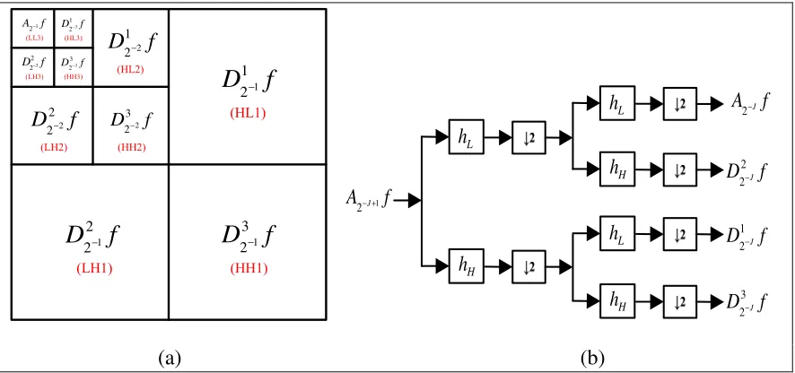
[image:36.612.104.547.156.364.2](a) (b)
Fig. 4. (a) Multiresolution image representation, (b) Analysis filter bank.
In 2-D the orthonormal basis is acquired using three wavelets ψ1(x),ψ 2(x),ψ 3(x),
where each of these can be considered to be the impulse response of a BPF with a certain
orientation preference. Thus the approximation A2jf of a signal f(x,y)at a scale
j
2 and
its information difference with A2j+1f are given as:
(
)
(
2)
( , ) 22 2 , 2
~ * ) , ( Z m n j j m y n x y x f f
A j j ∈
− −
− −
= θ (23)
(
)
(
2)
( , ) 21 1
2 ( , ), 2 , 2
Z m n j j m y n x y x f f
D j j
∈ −
− − −
= ψ (24)
(
)
(
2)
( , ) 22 2
2 ( , ), 2 , 2
Z m n j j m y n x y x f f
D j j
∈ −
− − −
= ψ (25)
(
)
(
2)
( , ) 23 3
2 ( , ), 2 , 2 nm Z
j j m y n x y x f f
D j j
∈ −
− − −
Here D jf 1
2 (HL) and D j f 2
2 (LH) correspond to the vertical and horizontal high frequencies
respectively, while D j f 3
2 (HH) corresponds to high frequency components in both
directions, represented in Fig. 4(a). However it must be noted that in Fig. 4 the scales are
in terms of 2− , >0
J
J where0≥ j≥−J.
Practical implementation of multiscale image decomposition has been done
effectively using filter banks. A filter bank is defined as an array of filters utilized to
separate a signal into various sub bands, generally designed in a manner to facilitate
reconstruction of the signal by simply combining the acquired sub bands. The
decomposition and reconstruction procedures are better known as analysis and synthesis
respectively. Fig. 4(b) and Table 1(below) portray the analysis filter bank and the
Daubechies 9/7 analysis coefficients (rounded to 16 digits) in the JPEG2000 compression
scheme [36], employed for multiscale analysis in the MAPGSEG algorithm.
TABLE 1: Daubechies 9/7 analysis filter coefficients
Low Pass Filter
High Pass Filter
0
0.6029490182363570
1.1150870524569900
±1
0.2668641184428720
-0.5912717631142470
±2
-0.0782232665289878
-0.0575435262284995
±3
-0.0168641184428749
0.0912717631142494
±4
0.0267487574108097
i hL(i) hH (i)
2.3 CIE 1976 L*A*B* COLOR SPACE
In 1976 the Commission International de l’Eclairage (CIE) proposed two device
independent approximately uniform color spaces, L*a*b* and L*u*v*, for different
important objective these color spaces were able to achieve with reasonable consistency
was that, given two colors, the magnitude difference of the numerical values between
them was proportional to the perceived difference as seen by the human eye [37].
Experimental data was used to model the response of a person through tristimulus values
X, Y and Z, which are linear transformations from R,G and B. Using these tristimulus
values the CIE L*a*b* was defined as:
16 116 * − = n Y Y f
L (27)
− = n n Y Y f X X f
a* 500 (28)
− = n n Z Z f Y Y f
b* 200 (29)
where ≤ ≤ + ≥ = α α x x x x x f 0 8276 1379310344 . 0 787 . 7 ) ( 3 / 1
,α=0.008856 , andXn, Yn and Zn are the
Chapter 3: PROPOSED ALGORITHM
The MAPGSEG algorithm embodied in six modules is shown in Fig. 5. The first
module (M1) is utilized to adaptively generate thresholds required for initial clustering
and region growth at varied levels of the input image pyramid. The second module (M2)
performs dyadic wavelet decomposition for multiresolution or pyramidal representation
of the input image. The third module (M3) carries out a progressively thresholded growth
procedure involving distributed dynamic seed addition. Module4 (M4) is responsible for
identifying transferable regions from one resolution to another by exploiting the interim
results as a-priori information. Texture modeling utilizing color quantization and entropy
computation, is performed in Module5 (M5). The proposed algorithm culminates in a
region merging module (M6) fusing the texture characterization channel and current fully
grown seed map, to give interim segmentations at low resolutions, and the final
segmentation map at a dyadic scale equal to that of the original input image.
Furthermore, it is imperative to note that the algorithm does not employ all modules at
every scale of the input image pyramid (observe the color coding legend in Fig. 5). The
Adaptive Gradient Thresholding Wavelet Decomposition
M1
M2
RGB2L*a*b* & Color GradientCurrent Dyadic Scale (Channel & Resolution
Information Storage)
Original Input Resolution ONLY
Resolutions EXCEPT Original Input
All Resolutions Processing at:
M3
M5
M4
M6
Progressive Region Growth & DistributedDynamic Seed Addition Texture Modeling Region Merging Seed Transfer INTERIM Segmentation FINAL Segmentation
0 20 40 60 80 100 120
[image:40.612.136.512.111.649.2]0 2000 4000 6000 8000 10000 12000 Gradient values N u m b e r o f p ixe ls Level2: 81X121 Level1: 161X241 Level0(Full Resolution): 321X481 Initial Clustering-MAPGSEG Progressive Region Growth-MAPGSEG
3.1 ADAPTIVE GRADIENT THRESHOLDING
The GSEG algorithm Version2.2 (V2.2) developed by Ugarriza et al. [33] utilized
fixed thresholds for segmentation, in the RGB color space. Initial clustering was
performed using a threshold value of 10, followed by a region growth procedure carried
out at thresholds intervals of 15, 20, 30, 50, 85, and 120. These fixed thresholds were
utilized for any image irrespective of its content, and intuitively can be deemed non-ideal,
owed to the varied gradient composition present in natural images. This intuitive notion
was substantiated as the fixed thresholds intervals were found to consistently pose major
problems that hindered the performance of the algorithm, clearly demonstrated by the
images in Fig. 6.
0 20 40 60 80 100 120 140 160 180 200 0
0.5 1 1.5 2 2.5
x 104
0 20 40 60 80 100 120 140 160 180 200 0
1000 2000 3000 4000 5000 6000 7000 8000 9000
0 20 40 60 80 100 120 140 160 180 200 0
1000 2000 3000 4000 5000 6000 7000
[image:41.612.111.541.364.682.2]3.1.1 EFFECTS OF STATIC THRESHOLD INTERVAL SELECTION
In Fig. 6 three natural scene images with their corresponding enhanced gradient map
histograms, are shown. In addition marked in green and red along each of the histograms
are the fixed threshold intervals utilized for initial clustering and region growth
respectively. Enhanced gradient maps are obtained by computing the gradient utilizing
the algorithm in [34] on the increased and decreased contrast versions of the original
RGB inputs and finding the pixel by pixel maximum among the two. Increased contrast
enhances dark regions and exposes edges present in these regions. On the contrary
decreased contrast exposes edge information present in bright areas of the image. Thus,
the maximum of the two yields a gradient map consisting of most edge information
present in the image. Although gradient map enhancement (employed in V2.2) is useful it
comes at the expense of increased computation, especially for large resolution images.
In Fig. 6 it can be observed that the varying shape of gradient histograms from image
to image causes the fixed thresholds to be distributed erratically without following a
uniform pattern, resulting in contrasting segmentation results. One way of analyzing the
effects of static threshold interval selection is by comparing the gradient content of the
images in each interval. Considering the first two intervals for region growth, from 10 to
15 and 15 to 20, we see large gradient content in the ‘Cheetah’ and ‘Cars’ images within
these intervals, and in contrast for the ‘Parachute’ image the content is small which may
result in over segmentation of flat regions with higher computational costs. In addition,
V2.2 was designed such that, only seeds (a labeled collection of pixels corresponding to a
particular region) which satisfy a certain minimum size criterion based on the current
seeds generated in these low gradient intervals, in the parachute image may be discarded,
rendering the thresholds constituting this interval to have negligible contribution to the
final segmentation result. Conversely, if an interval is very large in comparison to the
extent or span of the histogram, it causes regions with significantly different gradient
detail to be merged together, providing a segmentation that is incoherent with the original
input image (under segmentation).
Moreover, in Fig. 6(a) and 6(b) the span of the histogram both cases is smaller than
the final region growth threshold (120) resulting in wasted computational costs,
significantly effecting the overall performance of the algorithm. Thus, overcoming these
problems necessitated an adaptive thresholding approach based on image content.
3.1.2 ADVANTAGES OF CIE L*A*B* OVER RGB
The MAPGSEG employs adaptive gradient thresholding in the CIE 1976 L*a*b*
color space. The algorithm begins with a conversion from RGB to CIE L*a*b for correct
color differentiation, owed to the fact that the latter is better modeled for human
perception and is more uniform in comparison to the RGB space. The L*a*b* data is
8-bit encoded to values ranging from 0-255 for convenient color interpretation and to
overcome viewing and display limitations. In addition it has also been widely used for
commercial applications. The resultant color converted data is utilized for computing the
vector color gradient utilizing the previously mentioned algorithm described in [34],
without any enhancement methodology. In general for an image, 8-bit L*a*b* values
were found to span over a much smaller range than 8-bit RGB, consequently resulting in
0 20 40 60 80 100 120 140 160 180 200 0
0.5 1 1.5 2 2.5 3 3.5 4 4.5
x 104
Enhanced RGB CIE L*a*b*
0 20 40 60 80 100 120 140 160 180 200 0
5000 10000
15000 Enhanced RGB
CIE L*a*b*
0 20 40 60 80 100 120 140 160 180 200 0
2000 4000 6000 8000 10000
12000 Enhanced RGB
[image:44.612.110.536.70.403.2]CIE L*a*b*
Fig. 7. Gradient histogram RGB vs. CIE L*a*b* of: (a) Parachute, (b) Cheetah, (c) Cars.
In Fig. 7(a), 7(b) and 7(c), shown are the histogram comparisons of RGB (in blue)
and L*a*b*(in red), along with the color converted equivalents for the three images in
Fig. 6. It can be observed that the red curves are squeezed versions of the blue curves,
where the span of the red curves are significantly smaller than the ones in blue but the
amplitude of the red are much larger in comparison. To this effect, if we limit our
thresholds to the span of the histogram, this squeezed property is an advantage as the
region growth procedure is now confined to a significantly smaller range and for any
arbitrary threshold interval in this reduced range a higher number of pixels are worked
has enabled distinct differentiation between the chromatic and achromatic regions,
presenting the algorithm with this additional piece of information.
3.1.3 ADAPTIVE THRESHOLD GENERATION
The MAPGSEG algorithm is initiated with a color space conversion of the input
image from RGB to CIE L*a*b* for reasons specified in Sections 2.3 and 3.1.2. Using
the resultant L*a*b* data, the magnitude of the gradient G(i, j) of the full resolution
color image field is calculated. The threshold values required for segmentation are
determined utilizing the histogram of the color converted gradient map.
At first, the objective is to select a threshold for the initiation of the seed generation
process. Preferably, a threshold value should be selected to expose most edges while
ignoring the noise present in images. However, accomplishing this task is precluded by
the unique disposition of natural scene images, where a threshold that correctly
demarcates the periphery of a given region may unify other regions. Due to this factor,
we initiate our thresholding algorithm by estimating a value λ that aids in selecting the
regions without any edges or with extremely weak and imperceptible edges. We estimate
this threshold primarily based on the span of the histogram in combination with empirical
data. Given an image, we propose choosing one of two empirically determined threshold
values for initiating the seed generation process, by validating how far apart the low and
high gradient content in the image are, in its corresponding histogram. The idea is that a
high initial threshold be used for images in which a large percentage of gradient values
spread over a narrow range and a low initial threshold value be used for images in which
of the histogram. The choice of λ made in such a manner ensures that significant low
gradient regions are acquired as initial seeds.
0 10 20 30 40 50 60 70 80 90 100 0
[image:46.612.178.470.126.356.2]2000 4000 6000 8000 10000 12000
Fig. 8. Histogram based adaptive gradient thresholding
From a practical implementation standpoint, we made this decision of selecting the
initial threshold by obtaining the percentage ratio of the gradient values corresponding to
80% and 100% area under the histogram curve, as shown in Fig. 8. If 80% area under the
histogram curve corresponds to a gradient value that is less than 10% of the maximum
gradient value in the input image, a high threshold value is chosen else a low initial
threshold value is chosen. Keeping in view the problems posed by over and
under-segmentation, the low and high threshold values were empirically chosen to be 5 and 10
respectively. The former case was used for images where background and foreground
have largely indistinguishable gradient detail from each other. The latter case was used
for images consisting of a slowly varying background with less gradient detail, well
distinguished from prominent foreground content. Having obtained λ, all significant flat
varied size criterions, to form the initial seeds map. Once the threshold for initiating the
segmentation process is determined, we proceed to calculate thresholds intervals for the
dynamic seed addition portion of the region growth procedure.
Dynamic seed generation is that portion of the growth process where additional seeds
are added to the initial seeds at the lowest resolution or existing high confidence seeds at
subsequent higher resolutions. These threshold limits constituting various intervals
selected for region growth are determined utilizing the area under the gradient histogram
that does not fall within the g