School of Economics and Finance
Aid and Growth in Malawi
Daniel Chris Khomba and Alex Trew
Aid and Local Growth in Malawi
∗
Daniel Chris Khomba
†and Alex Trew
‡February 1, 2019
Abstract
We study the local impact of foreign aid to constituencies and districts in Malawi over the period 1999–2013 using a highly detailed new aid database that includes annual disbursements at each project location. First, we show using household panel surveys that growth in light density is a good proxy for growth in per capita consumption. Second, we introduce a new political dataset that permits novel instrumental variables. Using two instruments, together or separately, we find a consistent, robust and quantitatively significant role for aid in causing growth in light density. Constituency-level regressions point to a larger effect than at district level, suggesting that aid causes some relocation of activity across space but not enough to make the net effect zero. The impact on growth peaks after two to three years but then falls to zero, implying that foreign aid has a level effect on incomes but does not stimulate sustained growth. Bilateral aid appears to be better in causing growth than multilateral aid. Aid delivered as a grant has an impact while that given as a loan does not.
JEL Classifications: F35, O19, O55, R11.
Keywords: Foreign aid, economic development, favoritism.
∗We are grateful to Nicholas Crafts, Nathalie Ferri`ere, Stephan Heblich, Margaret Leighton, Bradley
Parks, Luigi Pascali, Jon Temple, Jessica Wells and seminar participants at St Andrews, the College of William & Mary and at the 2017 CSAE conference for helpful comments and discussion. Remaining errors belong to the authors. Khomba thanks the University of St. Andrews for PhD funding through a 600th Year Celebration Scholarship.
†School of Economics and Finance, University of St. Andrews, Email: dck2@st-andrews.ac.uk. ‡For correspondence: School of Economics and Finance, University of St. Andrews, St. Andrews,
1
Introduction
Evidence to support the hypothesis that development assistance stimulates economic
growth has been limited but growing over the last ten years.1 The search for a causal role for aid at a country level has long been bedevilled by problems of identification (see Qian,
2015). Since the allocation of aid can be related to the growth rate of the recipient it is
necessary to isolate exogenous variation in aid to establish a causal connection. Recent
country-level contributions, such as Galiani et al. (2017), have found an economically and
statistically significant role for aid in causing growth.
Aid is not uniformly distributed within a recipient country, however. Given the
impor-tance of urbanization and industrialization to growth, it could be informative to examine
the disaggregated aid disbursement pattern and the spatially proximate consequences for
growth. Recent efforts to use regional instruments (Dreher and Lohmann, 2015) have
found limited evidence of a any causal effect on regional growth as measured by nighttime
light data. That aid matters at a national level, but apparently not at a regional level,
presents a puzzle.
In this paper we evaluate the effectiveness of aid flows to different regions (both
parlia-mentary constituencies and administrative districts) in Malawi over the period 2000–2013.
We use two determinants of the internal distribution of development aid2 that are based on the political, institutional and cultural environment in Malawi. Our instruments
ex-ploit the Presidential powers to influence the disbursement of the Malawian development
budget. In general, one concern might be that this President-influenced spending carries
with it much more than foreign aid. However, in Malawi, foreign aid comprises nearly
three quarters of the discretionary budget over the period studied here. In district-level
regressions, we can also control for overall public spending and still find a significant,
causal role for aid. We can thus be confident that growth effects generated by the
dis-cretion exercised by the President is primarily due to the internal variation in foreign aid
flows. Our first instrument is a variable for ethnic affinity that is measured as the
pro-1See, for example, Boone (1996), Easterly et al. (2004), Rajan and Subramanian (2008), Doucouliagos
portion of a constituency or district population that is co-ethnic with the president. One
concern with this instrument might be that the ethnicity of the President is related to
those areas that anticipate future growth and so vote for a co-ethnic President; we show
using Malawian electoral records that there is no significant voting along ethnic lines. The
second instrument ispolitical switching measured as a dummy equal to one if the Member
of Parliament (MPs) in a constituency defects to join the party of the ruling President. In
district level regressions, this is the share of the district’s MPs that defect. As we argue
below, the likelihood of defection is unrelated to expected future growth. Using each of
these instruments, and both combined, we find economically and statistically significant
evidence on the effectiveness of aid in causing growth (as proxied by the log change in
nighttime light intensity which, as we show using household surveys, is strongly correlated
with the growth of household consumption). The growth impact of aid is quantitatively
significant and robust to local and year fixed effects, as well as a number of time-varying
controls. We show that the effect on growth is hump-shaped (with a peak at a lag of two
to three years), declining to zero over time. Aid for agriculture and education projects is
the most beneficial while multilateral aid appears to be less effective than bilateral aid.
Our use of these instruments is related to recent work on political favoritism. Hodler
and Raschky (2014) document the existence of regional favoritism in 126 countries. That
study finds a significant effect of a leader’s birthplace on the log of the average lighttime
night in a region. It also finds a positive interaction between aid and birthplace, which
Hodler and Raschky interpret as aid exacerbating the extent of favouritism. De Luca
et al. (2018) shows just how significant the role of co-ethnicity is in the allocation of
public funds in countries around the world. There are a number of difficulties in using
favoritism to instrument for aid, however. First, in many countries the aid budget is only
a small portion of the total discretionary budget being influenced by the political elite.
Favoritism may thus capture the allocation of non-aid spending and bias the measured
effect of aid on growth. Second, regions that vote for a particular leader may do so with
the expectation of returns – co-ethnic support for a President may be on the back of
explicit campaign promises of post-election investment. Third, using birthplace of the
where Presidents can remain incumbent for extended periods.
A number of features of Malawi over the period 2000–2013 help us address these
concerns. First, aid comprises a substantial portion of the budget controlled by the
President. Over our period of study, aid is 73% of development expenditures in Malawi.3 As we argue below, non-development expenditures are not subject to the same Presidential
interference. Second, we show that votes in Malawian elections are not historically along
ethnic lines. Third, the political environment over our study period is particularly volatile
with three different Presidents and three different ruling parties. As a result, we have
substantial variation over time in both of our instruments.
This study makes use of two key datasets. The first is of sub-national allocation
of foreign aid projects which comes from Malawi’s Aid Management Platform (AMP).
AMP contains 623 different projects from 43 different donors comprising US$7.1 billion
in aid (which is 82% of the total over our period). The AMP was initially based on
AidData (see Peratsakis et al., 2012), since it was created using data collected during
the geo-coding exercise conducted in conjunction with AidData. A benefit of using the
AMP is that it contains annual figures (commitments and disbursements) as well as the
planned implementation period as per the project contract. AMP data also includes
information on the project intention (i.e., support of agriculture, health or education)
which allows us to disentangle the effects of aid. The data also takes into account project
extensions or modifications (to, for example, project length or locations). We thus have an
exceptionally high level of information on actual annual disbursements of aid. The second
set of data is nighttime light data which is used to proxy for economic activity. There is
a growing literature that finds nighttime light images can be used as a proxy for output
growth and correlate well with other GDP-based measures of economic growth.4 For Malawi in particular, we use the World Bank’s Integrated Household Surveys to show that
there is a high correlation between district-level growth in average real annual household
consumption and district-level growth in light density. In addition to these data, we use
district and year fixed effects as well as employing a wide range of district-level controls,
3Data from Ministry of Finance’s annual Financial Statements.
4See Henderson et al. (2012), Michalopoulos and Papaioannou (2013), Lowe (2014) and Storeygard
including population density, non-development public expenditure, the poverty rate and
rainfall. We also control for a variety of measures of development need, such as gross
primary school enrolment, the number of classroom buildings, life expectancy, and infant
mortality as well as the number of people in a district that are food insecure.
Our contribution is related to the existing body of literature on aid effectiveness.
After the early work of Boone (1996), cross-country studies have used instruments such as
population size (Burnside and Dollar, 2000; Rajan and Subramanian, 2008) or bilateral
relationships (Bjørnskov, 2013). However, these approaches suffer from possibly direct
effects on growth (see Bazzi and Clemens, 2009; Dreher et al., 2013). Temple and Van de
Sijpe (2017) studies the consequences of aid for macroeconomic ratios. They find that
aid increases consumption and has an impact on investment with a lag. Galiani et al.
(2017) uses a convincingly excludable instrument and identifies a sizeable impact of aid
on real per capita growth. Studies at a regional level have found mixed evidence of a
causal effect of aid on growth. To address causality, Dreher and Lohmann (2015) use
an interaction between a country’s crossing of the IDA threshold and a measure of the
region’s historical probability of receiving aid (see Nunn and Qian, 2013). Dreher and
Lohmann find no effect of aid when using this instrumental variable. Dreher et al. (2016),
in contrast, does find a role for aid in causing growth at the regional level of Chinese aid
flows when using an interaction with Chinese steel production as instrumental variable.
Dreher et al. (forthcoming) find that the effect of short-term political favoritism at a
country level reduces the effectiveness of aid. Our estimates of the effect of aid may be
lower bounds for the true causal role played by aid.
There are recent papers that consider the impact of aid in Malawian regions.
Ra-jlakshmi and Becker (2015) investigates the allocation and effectiveness of geo-coded aid
projects from 30 agencies over 2004-2011. They find that aid reduces disease severity and
diarrhoea incidence while it also increases school enrolment. Dionne et al. (2013) also use
co-ethnicity to understand the allocation of aid across districts. In their study, aid has a
limited impact on health and education outcomes.
Our study is also related to the literature on the ethnic and political distribution of
Hodler and Raschky (2014) find evidence for the importance of ethnicity in the distribution
of resources (including development aid). A growing literature following Alesina and
Dollar (2000) has found a role for political influence in both the distribution of aid and in
diminishing its effectiveness in generating development (see, for example, Dunning, 2004;
Heady, 2008; and, Jablonski, 2014). We use these insights in the particular context of
Malawi to motivate our instruments.
The rest of this paper is organized as follows. We discuss the Malawian political
and economic context in Section 2. In Section 3 we introduce the data and develop our
empirical strategy in section 4. Section 5 presents our main results first at the level of
193 constituencies and then at the level of the 28 administrative districts. Constituency
regressions permit us to cluster standard errors at the level of the district, while district
regressions allow us to use a wider set of controls. Section 6 considers the effect of aid
by project type and investigates the dynamic effects of aid. Finally, Section 7 offers some
concluding remarks.
2
Malawi
Malawi is a landlocked country in South Eastern Africa with a population in 2015 of 17.2
million (up from 3.6 million in 1960). With few natural resources, 85% of its population is
rural and relies upon small-scale subsistence farming of the staple food (maize). Over 29%
of GDP comes through exports and over half of that export revenue comes from one crop
(tobacco). Malawi has historically suffered from high poverty, poor health outcomes and
volatile growth. Nearly half (47.8%) of children under five years of age are malnourished
according to stunting data (the average for sub-Saharan Africa is 39.9%. Based on figures
from 2010, 70.9% of the population live below $1.90 a day (2011 PPP).5 The 2015 United Nations Human Development Index (HDI) ranked Malawi 173rd out of 186 countries.
5Data from Malawi National Statistical Office (NSO), World Bank, and the Human Development
Foreign Aid
Given the low tax base, and the susceptibility to domestic supply and international
de-mand shocks, foreign aid has constituted a significant proportion of government
expen-ditures. Over 40 multilateral and bilateral development partners6 have contributed an average 40% of the national budget over the last decade (Malawi Government (2011)).
Figure 1 depicts ODA7 per capita (panel a) and aid as a share of GNI (panel b) for Malawi against the average for Sub-Sahara Africa (SSA) and the average for Low Income
Countries (as defined by the World Bank for the World Development Indicators). As can
be seen, the per capita trend in aid flow to Malawi has followed that to other LICs but,
since it is one of the poorest, aid as a share of income is relatively high. The majority of
aid goes to health, education, agriculture and governance. Over the period of study, 8%
of assistance has been given as humanitarian (non-development) aid.
Politics and spending
Malawi is divided into 28 administrative districts with the capital in Lilongwe. Following
independence from British colonial administration in 1965, Malawi was for nearly three
decades a one-party State. Since 1993, Malawi has been a multi-party democracy with a
Parliament and President elected every five years. As can be seen in Figure 2, elections
have regularly resulted in a change of President and party. However, as typical in many
African countries, a ‘Big Man’ syndrome persists in Malawi – the President has significant
discretionary power and tends to favour a group of trusted co-ethnics (see Francois et al.,
2012). Some of the resources of the State are the patronage of this powerful ruler. In a
country without any notable natural resources, state resources in Malawi means control
over bureaucratic positions, powers to allocate rents (including foreign aid), public services
and determine policies and their beneficiaries.
Important for the purposes of this paper is the nature of the political system as it
relates to control of expenditure. Public spending is divided into the recurrent budget
6Among these are USAID, the World Bank, the Global Fund (to fight HIV/AIDS, malaria and
tuber-culosis), the European Union (EU), and, more recently, China.
7ODA is technically the same as development aid, as classified by OECD. It excludes aid to
and the development budget. As we describe below, the Malawian development budget is
that portion of the public spending that is under the influence of the President and this
development budget is three quarters development assistance from overseas.
3
Data
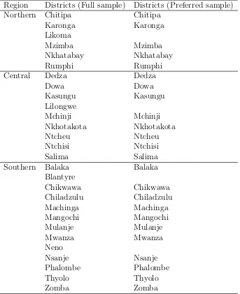
This study uses data available over the period 1999 to 2013. There are 193 constituencies
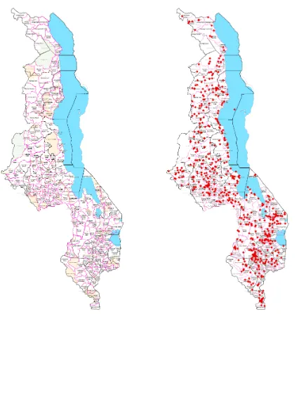
and 28 administrative districts in Malawi (see the left panel of Figure 3).8 In most specifications we omit those constituencies or districts that were recently formed or split.9 Further the two major cities of Lilongwe (the capital city) and Blantyre are omitted from
most estimations. In constituency regressions we also omit each district’s Boma (the
constituency in the district that hosts administrative office).
Data on projects financed by foreign aid is from the Aid Management Platform (AMP),
managed at the Ministry of Finance (MoF) in Malawi. The AMP is the government’s main
tool for tracking and reporting progress of aid-funded activities in Malawi and began with
AidData’s Malawi Geocoding Project which was the first effort to compile comprehensive
geocoded data of all donor activities in a single recipient country in Africa. Based on
information reported by both donors and the Malawi Government, the AMP contains
geocoded data on projects from over 40 donor agencies covering 623 projects across 706
project locations. These projects total $7.1 billion (82% of total foreign aid to Malawi
between 2000 and 2013). Figure 3 (right panel) shows a map of Malawi with the geocoded
projects. The AMP data disaggregates cumulative project totals into annual commitments
and actual disbursements of each project in a particular district. For this study, we use
actual disbursement figures. Those projects in the AMP without location information
have been excluded, reducing the number of projects used in this study to 593 projects.
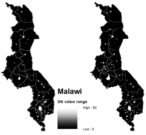
To proxy for economic growth we use nighttime light data.10 Geographers (Elvidge
8Table 1 gives all data and sources used. Table 2 lists all the districts in Malawi.
9Neno and Likoma districts were formed after splitting from Mwanza and Nkhatabay districts
respec-tively. For these new districts, some data on most of the variables is missing not because they are not necessarily reported, but rather because for most of the years under study they were still being reported as part of the districts they were split from. Thus they are entirely excluded but they are subsumed as part of the parent districts.
et al., 1997; Sutton et al., 2007) and ecologists (Doll et al., 2006) first used light density to
study urbanization. Chen and Nordhaus (2011) and Henderson et al. (2012) subsequently
showed that light intensity at night is a good proxy for local economic activity. By
using luminosity, we have reliable data at high spatial resolution for those countries in
which data availability is otherwise limited. Among more recent examples of its use are
Michalopoulos and Papaioannou (2013), which studies development in Africa, and the
aforementioned Hodler and Raschky (2014). We use the light data with intercalibration
correction for sensor degration and orbital changes (see Elvidge et al., 2014).
A further advantage of basing our study on Malawian data is that we can check
our proxy for development using the World Bank Living Standards Measurement Study
in the years 2010, 2011 and 2013. The Integrated Household Surveys contain a great
deal of information including real annual household consumption. In Table 3 we report
correlations between the log level of light density and the district level average of the
log level real annual consumption per capita and per household. The correlation is high,
between 52 and 72%, and consistent across years. Moreover, the correlation between
average growth in real consumption and growth in light density is just as strong. The
correlation between the growth in light density and the growth in per capita consumption
is 0.53 over the period 2010–13.
Figure 4 depicts luminosity at the pixel level for Malawi in 1999 and 2010 against the
district borders.11 For analysis in this paper, we calculate average light density at the constituency or district level (average light intensity per square kilometer) in each year
over the period 1999 to 2013.
At constituency level, we use a number of additional controls including the log of
population and the poverty rate from the National Statistic Office (NSO) census reports.
Data on party affiliations of Members of Parliament, as well as list of Cabinet Ministers,
is from Parliamentary Hansards found at the Malawi National Assembly library. Rainfall
data is from meteorological reports provided by the 22 meteorological stations that form
the weather network in Malawi. District-level regressions permit a wider range of controls.
noaa.gov/eog/dmsp/downloadV4composites.html.
11Maps for administrative districts are downloaded from DIVA-GIS, available at
We include data on local public spending excludes aid (since aid is managed by central
government Ministries), infant mortality, life expectancy and rate of food insecurity are
from various reports from the NSO. Education data (gross primary enrolment and number
of primary school classroom buildings) is from the Ministry of Education, Science and
Technology. Table 1 gives a summary of the data used in the analysis and their sources
while Table 4 shows descriptive statistics of the variables in the baseline sample.
4
Empirical strategy
We wish to estimate a light density growth regression of the following form,
∆LDi,t =β0+β1LDi,t−1+β2Aidi,t−1+X0i,t−1β+µi+γt+εi,t (1)
where LDi,t is log light density in constituency/district i at period t, ∆LDi,t =LDi,t−
LDi,t−1,Aidi,t is the log of aid disbursements,Xis a vector of control variables andµi and
γt are constituency/district and time fixed effects. Robust standard errors are clustered
at the level of the district in constituency regressions, and at the level of the three regions
in district level regressions.
A first concern with the specification in equation (1) is that aid disbursements are
not random. In particular, we may expect that development assistance is given to those
areas with the lowest expected growth, or those that have suffered negative shocks in the
past. Conversely, it may be that, particularly within a country, assistance is given to
those areas that show the greatest potential for generating growth. Second, we may face
attenuation bias since we are using an imperfect proxy for economic activity. Third, there
may be unobserved variables related to both aid and development, that make the role of
aid appear significant.
To account for these concerns we employ two novel instruments that are related to the
discretionary powers of the President to favour those in his/her inner circle but are not,
we argue, related to development through other channels. We thus use our instruments
∆LDi,t =β0+β1Aiddi,t−1 +β2LDi,t−1+X0i,t−1β+µi+γt+εi,t, (2)
Aidi,t =α0+α1zi,t+α2LDi,t−1+X0i,tα+µi+γt+νi,t, (3)
where z is an instrumental variable. For the instrument to be valid, it must be relevant
(α1 6= 0) and exogenous (cov(zi,t, εi,t) = 0).
We discuss a number of potential concerns about the validity of each of these
instru-ments below. One issue that is common to each regards the nature of the discretionary
powers that the President has. It may be that the President allocates a large portion of
State resources in addition to foreign assistance. In many countries, this would be a valid
concern but, by focusing on Malawi, it is less problematic. The Malawian Development
Budget is that portion of the public spending that is under the most influence of the
President. Other departmental expenditure is comprised of recurrent expenses such as
salaries, interest payments on public debt, procurement of goods and services, payment
of pensions and gratuities, etc. There is limited scope for the President to exert
discre-tion on the allocadiscre-tion of these budgets across districts. The allocadiscre-tion of transfers to
districts is determined by the National Local Government Finance Committee (NLGFC)
– a quasi-governmental institution mandated with effective mobilization, equitable
distri-bution and efficient utilisation of financial resources in local councils. Finally, in Malawi,
the Development Budget is 73% foreign aid over the period of study.
Ethnic affinity as instrument
Our first instrument is the proportion of the population in a district or constituency that
is co-ethnic with the sitting President. Malawi people are of Bantu origin and comprise
many different ethnic groups. Malawi Human Rights Commission (2005) finds that there
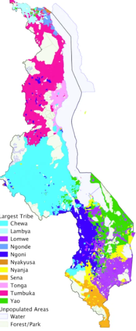
are about 15 ethnic groups in Malawi. The major ones are shown in Figure 5. The largest
group, the Chewa people, make up 38.4% of Malawi’s population and are mainly found
in the center. As shown in Figure 2, over our study period the President is either Lomwe
The relevance condition requires that the instrument be a predictor of aid
disburse-ments. There is already evidence that disproportionate amounts of aid are allocated to
an incumbent President’s district of birth, especially in Sub Saharan Africa. Franck and
Rainer (2012) use data from 18 African countries over 50 years and find significant
ev-idence of large and widespread ethnic favoritism in the allocation of aid resources. As
an example of this in Malawi, Figure 6 shows district-level aid disbursements in Malawi
under two Presidents of different ethnic origins. Despite the fact that President Bakili
Muluzi received a majority of votes in districts in the Southern region, the Yao districts
of Machinga (his birth district), Mangochi and Balaka are allocated disproportionately
higher amounts of aid than any of the other districts. When President Bingu wa
Muntha-lika of Lomwe origin was in office, and despite getting a bigger share of votes in the Yao
districts than he got from his birth district, Figure 6 shows that the Lomwe districts of
Thyolo, Mulanje and Phalombe received more aid than the Yao districts.
One concern with the exogeneity of this instrument relates to the connection between
co-ethnic voting behavior. There is a large literature on the role of ethnicity in African
voting behavior (see, for example, Posner, 2005). If districts supported Presidential
can-didates primarily along ethnic lines then a President’s ethnicity ceases to be random – a
district’s vote is for the candidate that will send the aid their way. If it is the poorest
districts that most vote along ethnic lines, then our instrument is not exogenous.
There is evidence against this clientelistic interpretation, however. Recent studies in
Ghana (Lindberg and Morrison, 2008) and South Africa (Anyangwe, 2012) find no or
very limited evidence that voting is subsumed in ethnicity. For Malawi, we report in
Appendix Table 12 results from a regression of the vote share that a winning candidate
received from each district in the 1999, 2004 and 2009 general elections on the proportion
of the winning candidate’s co-ethnics in a district. Ethnicity does not seem to affect the
vote share that a candidate gets in the district, being found to be statistically
insignif-icant. In contrast, party identification, a dummy variable that takes the value 1 if the
winning President’s party has a parliamentary majority in that district, or 0 otherwise,
is statistically significant.
ethnicity could affect the level of economic activity at the district level. For instance, it
may be that the cultural practices of a particular ethnic group are more consistent with
higher economic activity. To account for this possible channel, for each of the five largest
ethnic groups we include a dummy variable equal to 1 if a given district has a majority
of that ethnicity.
Political switching as instrument
Another determinant of aid distribution can be the desire of the incumbent President
to consolidate their political base. There is evidence that aid is distributed towards
electorally-strategic regions and away from opposition dominated regions (Briggs, 2012;
Jablonski, 2014). Our second instrument is thus the proportion of Members of
Parlia-ment (MPs) in a district that defect from the political party with which they won the
Parliamentary seat to the party of the ruling President. In constituency regressions this
is a dummy variable (i.e., the proportion is 1 if the constituency MP defects).
Political affinity is often viewed in a similar way as ethnicity in African politics.12 In this view, a leader is constrained in exercising full ethnic exclusion since doing so may
not adequately sustain a coalition of support. In order to consolidate their political base,
leaders look to co-opt other powerful elites, often from ethnic groups in regions distinct
from their own. In Malawi, this co-opting often takes the form of defection (‘crossing the
floor’) rather than the formation of cross-party coalition governments. As in many
Sub-Saharan countries, once the President is in power the biggest barrier to total control is not
having a majority representation in Parliament. Defection is induced by the promise of
personal gains (i.e., public office) and a flow of aid to the defecting MP’s region. Districts
that gave the President only limited electoral support may now be favored with aid flows.
Crossing the floor comes with risk for the politician, however. First, Section 65 of
the Malawi Constitution prohibits MPs from crossing the floor. This is intended to keep
the composition of Parliament close to that determined by the vote. By crossing the
floor, they risk their seats being declared vacant. Second, defection reduces the chances
of being re-elected in the next general election. As discussed, party identification is key
to voter behavior. By defecting, an MP is generally joining a party that does not have a
stronghold in their own district. For example, of the 68 MPs that defected to the DPP
in 2005, 35 MPs came from districts in the Central and Northern regions where the DPP
did not have wide support. Of these, 32 seats were contested in the 2009 general elections
for the DPP and 21 lost their seats.
Despite the possible costs of defection it has happened frequently in Malawi, especially
over the period 2005 and 2012. The need to consolidate political power can emerge when
coups threaten, when a sitting President dies or when the ruling political party is changed
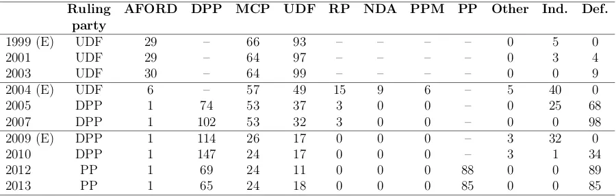
without an election. Table 5 provides the breakdown of the composition by party of
Malawi’s Parliament. The period of volatility since 2005 was the result of non-electoral
events. In 2005, Dr Bingu wa Munthalika formed the Democratic Progressive Party
(DPP), abandoning the United Democratic Front (UDF) on whose ticket he contested in
the 2004 elections. The DPP became the ruling party and the UDF, which had won the
2004 elections, became part of the opposition. In 2011, the then Vice President Dr Joyce
Banda formed a new party, the Peoples Party (PP), abandoning the DPP with which she
was Dr wa Munthalika’s running mate in 2009 elections. Upon Dr wa Munthalika’s death
in 2012, she assumed the presidency and her PP became the ruling party while the DPP
moved to opposition.
An example of the impact of the reconstitution of parties on aid disbursement is the
period from 2004–2005. When Dr wa Munthalika abandoned the party with which he
was elected president in 2004 (UDF) to form his own DPP in 2005, the DPP initially had
no MPs in Parliament and had difficulties in passing policies and legislations. Through
inducing defections, the DPP managed to co-opt MPs particularly from the Northern
districts (see figure 7). As can be seen in figure 6, from 2005 some of these Northern
region districts received significantly more aid disbursement than before.
For this instrument to be valid, we require that the likelihood of an MP’s defection is
unrelated with future economic growth in the constituency they represent. The motivation
to defect depends on the type of defector. Independent MPs are generally the first to be
to make quick and easy personal gains, though some may even be appointed into key
positions. As the Table 5 shows, almost immediately after each election, the number
of independent MPs reduce to rapidly to 0 in subsequent years (from 40 in 2004 and
from 32 in 2009). Figure 7 shows that many of the newly DPP regions were formerly
independent. A second type of defector is an influential, veteran MP that has already
served for a long period. For these power brokers, where they lose their positions when
the President changes, promise of re-appointment into the positions that accord them
powers, and development assistance in their district, induces their switching of parties. A
third type of defector is a member of a smaller or breakaway party. Table 4 shows that
the number in ‘Other’ is generally nonzero in an election year but declines to zero once
the winning party attracts them to defect. During 2004 election, National Democratic
Alliance (NDA), which broke away from the UDF after a leadership dispute, won 9 seats
and Peoples Progressive Movement (PPM) (another party formed from disputes) won 6
seats, however by 2005 when the DPP was formed and took power, they all defected and
joined the new ruling party.
5
Main results
We present results first at the constituency level and then at district level. Regressions at
constituency level benefit from a larger cross section and the ability to cluster standard
errors at the district level but limits the set of control variables. District level regressions
also permit a wider range of extensions, which we introduce in Section 6.
5.1
Constituency results
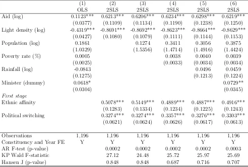
Table 6 reports results using both instruments at the constituency level. All regressions
include constituency and year fixed effects with robust standard errors clustered at the
level of the 24 districts. In Column 1 we report the OLS regression results using all
controls. The OLS result with all controls suggests a positive and statistically significant
connection between growth and the log of aid. Two-stage least squares results are in
of each instrument in the first stage regression is strong in all specifications. When we
instrument for the log of aid using political switching and ethnic affinity, the size of the
coefficient on aid increases and it is statistically significant at the 1% level across all
specifications in Columns 2–7.
As we would expect, the coefficient on initial light density is negative and significant
in all specifications, capturing a conditional convergence across districts. The log of
population and the log of rainfall are positively related with light density growth. The
poverty rate is not significant while a dummy for whether the constituency is represented
by a minister is generally significant. The log of aid disbursements is highly statistically
significant in all specifications.
Across all specifications, the Anderson-Rubin p-value is less than 0.01 and the F
-statistic for instrument exclusion is greater than 10. Thep-value of the HansenJ-statistic
is between 0.71 and 0.85, so we fail to reject the over-identifying restriction across all
spec-ifications. Results from regressions using only the ethnic affinity instrument are in
Ap-pendix Table 13; that from using only the political switching instrument are in ApAp-pendix
Table 14. Anderson-Rubin and KP statistics show that the instruments also perform
strongly individually.
Our preferred constituency-level specification is that in Column 6 of Table 6. This
implies that a 10% increase in aid disbursed to a constituency causes light density to
increase by 6.22% per year. The magnitude of the effect is larger than that found in
Galiani et al. (2017), although that study uses real GDP growth as a dependent variable.
While some of the effect of the aid disbursement may be to re-allocate activity across
space, the results from district-level regressions also support the finding that aid is causally
important.
5.2
District results
Table 7 reports results using both instruments at the district level. In addition to the
baseline controls used at the constituency level, we add the log of public spending since the
include district and year fixed effects. At the district level, the OLS regression with all
controls (column 1) suggests a positive but statistically weak connection between growth
and the log of aid.
Two-stage least squares results are in columns 2–9. The statistical significance of each
instrument in the first stage regression is strong in all specifications. When we instrument
for the log of aid using political switching and ethnic affinity, the size of the coefficient
on aid increases and it is statistically significant at the 1% level across all specifications
in Columns 2–9. The increase in the coefficient between OLS and 2SLS can be the result
of measurement error. This is common to recent studies on aid and growth (including
Dreher and Lohmann, 2015 and Galiani et al., forthcoming).
Public expenditure (excluding foreign aid) is insignificant, which is reassuring if we
are concerned that an affect on growth may operate through a President’s influence over
non-development spending. Districts with greater population density grow faster, which
is consistent with the literature on urbanization and development (see Desmet and
Hen-derson, 2015). The log of rainfall appears to play no role in explaining variations in
growth. Columns 3 and 4 add measures of education in districts. The log of the gross
primary enrolment rate is statistically significant in most specifications. The coefficient
on the number of classroom buildings is not statistically significant. Columns 5 and 6 add
health outcome variables while Columns 7 adds a measure of agricultural security.
Across all specifications, the Anderson-Rubin p-value is less than 0.01 and the F
-statistic for instrument exclusion is greater than 10. What is clear in the first stage results
is that the political switching instrument is less statistically significant at the district level.
This makes sense given we take the proportion of MPs that switch as our instrument; it
also suggests that there is limited within-district correlation in the likelihood of switching.
The p-value of the Hansen J-statistic is between 0.11 and 0.13, so we fail to reject the
over-identifying restriction across all specifications. Results from regressions using only
the ethnic affinity instrument are in Appendix Table 15; that from using only the political
switching instrument are in Appendix Table 16. Anderson-Rubin and KP statistics show
that the instruments also perform strongly individually.
in-crease in aid disbursed to a district causes light density to inin-crease by 1.9% per year, which
is smaller than in constituency regressions. The difference in the size of the coefficient
may result from aid causing some movement of economic activity across constituencies
within a district. Since the standard deviation of the log of aid is 1.1076, the effect of a
one standard deviation increase in aid disbursement is to increase light density by 21.4%.
The effect of aid on growth is, in absolute terms, quantitatively important for short-run
growth.
6
Extensions
Our dataset contains detailed information on the disbursements in each year of each
aid project, the type of project (agricultural, health and education) and the nature of
the funding body (whether a loan or a grant; whether multilateral or bilateral donor).
Moreover, one of the advantages of our identification strategy, is that it provides a way of
isolating the variation in aid disbursement to different districts over time. We can thus
look to understand impact of aid on growth over time.
Time lags
In a first extension, we look at the effect of aid on growth with a longer lag than one year.
To do so, we estimate the following system,
∆nLDi,t =β0+β1Aiddi,t−n+β2LDi,t−n+X0i,t−nβ+µi+γt+εi,t, (4)
Aidi,t−n =α0+α1zi,t−n+α2LDi,t−n+X0i,t−nα+µi+γi,t−n+νi,t−n, (5)
where ∆nLDi,t denotes LDi,t −LDi,t−n and n > 1. In other words, our estimate of β1 captures the effect of aid in time t−n on growth in light density over the subsequent n
years.
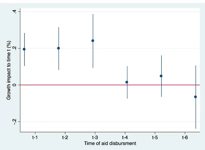
In Table 8, we add lags of up to six years to the constituency specification from Table
increasing over time until a peak effect on growth in light density after two years since
the aid was disbursed (that is, aid disbursed att−2 having an impact on growth between
t−2 and t). The effect declines thereafter, falling to close to zero at a lag of six years.
Table 9 and Figure 9 depict a similar story at the district level, although in this case the
(smaller) peak effect is seen after three years. Both the constituency and district results
suggest that there are real gains to aid, but that the effect on growth disappears after four
to six years. That is, aid appears to have a persistent effect on the level of light intensity,
but not on its growth rate.
Project type
Some aid projects in the AMP include information on the targeted outcome for the
fund-ing. Table 10 shows results for those projects that go to agriculture, health and education
(which together comprise 56% of total aid in the dataset). The performance of the
in-struments is mixed in some aspects, with limited strength in the first stage. The largest
coefficient is on aid to agriculture which makes sense given the direct importance of
agri-culture for the Malawian economy. The growth impact of aid for education and health
projects is lower, though it remains statistically significant at the 10% level.
Funding type
Table 11 reports results of the effect of aid on growth broken down into the type of funding,
multilateral or bilateral, grant or loan. The instruments work well in each of these types
of aid. Table 11 suggests that bilateral aid has a larger short-run impact on growth than
multilateral aid. Individual countries, particularly China, have increased bilateral aid
flows over recent years and these results suggest that the results from those projects in
terms of growth have been successful. Moreover, grants have a greater impact than loans,
suggesting that the expectation of future higher taxation may limit the contemporaneous
7
Concluding remarks
In focusing the disbursement of aid within one country, we have developed a new way of
isolating the causal relationship between the flow of aid and the rate of growth. We have
shown that there is a robust and qualitatively significant impact of aid on
contemporane-ous growth and a hump-shaped response up to two years after the initial disbursement.
The difference between the constituency and district results suggest that aid causes a
significant relocation of activity across space but that, nevertheless, the effect overall is
positive.
The identification strategy we employ is particular to the political and institutional
environment in Malawi. While there is evidence on the role of ethnicity (via birthplace)
in other contexts, the instrument based on attraction of political defections could also be
considered elsewhere. Malawi is among the poorest of the LICs, but the apparent success
of aid in causing growth in this country suggests that some of the pessimism regarding
aid effectiveness that has emanated out of the mixed empirical evidence in recent years
may have been misplaced.
Further study of the consequences of aid using geographically disaggregated data, with
particular attention to unbundling the different types of assistance, could significantly
improve our understanding of the effectiveness of foreign aid.
References
Alesina, A. and Dollar, D. (2000). Who gives foreign aid to whom and why? Journal of Economic Growth, 5(1):33–63.
Anyangwe, C. (2012). Race and ethnicity: Voters’s party preference in South African elections. International Journal of African Renaissance Studies - Multi-, Inter- and Transdisciplinarity, 7(2):38–58.
Arndt, C., Jones, S., and Tarp, F. (2010). Assessing foreign aid’s long-run contribution to growth and development. World Development, 69:6–18.
Arriola, L. R. (2009). Patronage and political stability in Africa. Comparative Political Studies, 42(10):1339–1362.
Bjørnskov, C. (2013). Types of foreign aid. University of Aarhus Working Papers, (2013-08).
Boone, P. (1996). Politics and the effectiveness of foreign aid. European Economic Review, 40(2):289–329.
Briggs, R. C. (2012). ‘Electrifying the base? Aid and incumbent advantage in Ghana’.
The Journal of Modern African Studies, 50(04):603–624.
Burnside, C. and Dollar, D. (2000). Aid, policies, and growth. American Economic Review, 90(4):847–868.
Chen, X. and Nordhaus, W. (2011). Using luminosity data as a proxy for economic statistics. The Proceedings of National Academy of Science, 108(21).
Dalgaard, C.-J. and Hansen, H. (2010). Evaluating aid effectiveness in the aggregate: A critical assessment of the evidence.
De Luca, G., Hodler, R., Raschky, P. A., and Valsecchi, M. (2018). Ethnic favoritism: An axiom of politics? Journal of Development Economics, 132:115–29.
Desmet, K. and Henderson, J. V. (2015). ‘The Geography of Development Within Coun-tries’. Chapter 22 in Duranton, G., J.V. Henderson and W. Strange. Handbook of Regional and Urban Economics, Elsevier.
Dionne, K., Kramon, E., and Roberts, T. (2013). Aid effectiveness and allocation: Evi-dence from Malawi. Paper Presentation at the ASA 2013 Annual Meeting.
Doll, C. N., Muller, J.-P., and Morley, J. G. (2006). Mapping regional economic activity from night-time light satellite imagery. Ecological Economics, 57(1):75 – 92.
Doucouliagos, H. and Paldam, M. (2009). The aid effectiveness literature: The sad results of 40 years of research. Journal of Economic Surveys, 23(3):433–461.
Dreher, A., Eichgenauer, V., and Gehring, K. (Forthcoming). ‘Geopolitics, Aid and Growth: The Impact of UN Security Council Membership on the Effectiveness of Aid’.
World Bank Economic Review.
Dreher, A., Fuchs, A., Hodler, R., Parks, B. C., Raschky, P. A., and Tierney, M. J. (2016). Aid on Demand: African Leaders and the Geography of China’s Foreign Assistance. AidData Working Paper 3.
Dreher, A., Klasen, S., Vreeland, J. R., and Werker, E. (2013). The costs of favoritism: Is politically driven aid less effective? Economic Development and Cultural Change, 62(1):157–191.
Dreher, A. and Lohmann, S. (2015). Aid and growth at the regional level. Oxford Review of Economic Policy, 31(3-4):420–446.
Easterly, W., Levine, R., and Roodman, D. (2004). New data, new doubts. American Economic Review, 94(3):774–780.
Elvidge, C. D., Hsu, F.-C., Baugh, K. E., and Ghosh, T. (2014). National trends in satellite-observed lighting 1992-2012. In Weng, Q., editor, Global Urban Monitoring and Assessessment through Earth Observation, chapter 6, pages 97–120. CRC Press: Taylor and Francis Group.
Elvidge, C. D., Kihn, E. A., Baugh, K. E., Kroehl, H., and Davis, E. (1997). Mapping city lights with nighttime data using dmsp operational linescan system data. Photogram-metric Engineering and Remote Sensing, 63:727–734.
Franck, R. and Rainer, I. (2012). Does the leader’s ethnicity matter? ethnic favoritism, education, and health in Sub-Saharan Africa. American Political Science Review, 106(02):294–325.
Francois, P., Rainer, I., and Trebbi, F. (2015). How is power shared in Africa? Econo-metrica, 83(2).
Galiani, S., Knack, S., Xu, L. C., and Zou, B. (2017). The effect of aid on growth: Evidence from a quasi-experiment. Journal of Economic Growth, 22(1).
Heady, D. (2008). Geopolitics and the effect of foreign aid on economic growth, 1970-2001.
Journal of International Develeopment, 20(2):161–180.
Henderson, J. V., Storeygard, A., and Weil, D. N. (2012). Measuring ecconomic growth from outer space. American Economic Review, 102(2):994–1028.
Hodler, R. and Raschky, P. A. (2014). Regional favoritism. The Quarterly Journal of Economics, 129(2):995–1033.
Jablonski, R. S. (2014). How aid targets votes: The impact of electoral incentives on foreign aid distribution. World Politics, 66(2):293–330.
Joseph, R. A. (1987). Democracy and prebendal politics in nigeria: The rise and fall of the second republic. African Study Series, 56.
Lindberg, S. I. and Morrison, M. K. C. (2008). Are African voters really ethnic or clien-telistic? Survey evidence from Ghana. 123(1):95–122.
Lowe, M. (2014). Rail revival in Africa? the impact of privatization. Joint RES-SPR Conference on Macroeconomic Challenges FacingLow-Income Countries: New Perspec-tives.
Malawi Government (2011). Malawi aid atlas, 2011 fiscal year. Technical report.
Malawi Human Rights Commission (2005). Report on cultural practices in malawi. Tech-nical report.
Michalopoulos, S. and Papaioannou, E. (2013). Pre-colonial ethnic institutions and con-temporary African development. Econometrica, 81(1):113–152.
Peratsakis, C., Powell, J., Findley, M., Baker, J., and Weaver, C. (2012). Geocoded Activity-Level Data from the Government of Malawi’s Aid Management Platform. Washington D.C. AidData and the Robert S. Strauss Center for International Secu-rity and Law.
Posner, D. (2005).Institutions and Ethnic Politics in Africa. Cambridge University Press.
Qian, N. (2015). Making Progress on Foreign Aid. Annual Review of Economics, 7:277– 308.
Rajan, R. G. and Subramanian, A. (2008). Aid and growth: What does the cross country evidence really show? The Review of Economics and Statistics, 90(4):643–665.
Rajlakshmi, D. and Becker, C. (2015). The Foreign Aid Effectiveness Debate: Evidence from Malawi. AidData Working Paper #6. Williamsburg, VA: AidData. Accessed at http://aiddata.org/working-papers.
Robinson, A. L. (2016). Internal Borders: Ethnic-based market segmentation in Malawi.
World Development, 87(C):371–384.
Storeygard, A. (2014). Farther on down the road: Transport costs, trade and urban growth in Sub-Saharan Africa. (0781).
Sutton, P. C., Ghosh, T., and Elvidge, C. D. (2007). Estimation of Gross Domestic Product at sub-national scales using nighttime satellite imagery. International Journal of Ecological Economics and Statistics, 8(S07).
Temple, J. and Van de Sijpe, N. (2017). Foreign aid and domestic absorption. Journal of International Economics, 108:431–43.
Van de Walle, N. (2007). Meet the new boss, same as the old boss? the evolution of political clientelism in Africa. In Kischelt, H. and Wilkinson, S. I., editors, Patrons, Clients and Policies: Patterns of Democratic Accountability and Political Competition, pages 50–67. Cambridge University Press.
A
Figures
Figure 1: Net aid to Malawi and other regions
(a) Per capita (current US$)
1995 2000 2005 2010 2015 20
40 60
(b) Share of GNI (%)
1995 2000 2005 2010 2015 10%
20% 30% 40%
Source: World Bank’s World Development Indicators.
—Malawi - - -SSA · · · LICs
Figure 2: Timeline of recent Malawian politics
President (ethnicity)
Muluzi
(Yao)
B. Mutharika
(Lomwe)
Banda
(Yao)
P. Mutharika
(Lomwe)
Party UDF DPP PP DPP
1994 election
1999 election
2004 election
2009 election
Figure 5: Spatial distribution of ethnic groups in Malawi
Figure 7: Map of political change in Malawi between 2004 and 2005
(a) Malawi political landscape 2004 (b) Malawi political landscape 2005
[image:30.595.133.470.486.741.2]B
Tables
Table 1: Data descriptions and sources
Variable Description Source Years
Light density Average nighttime light intensity per con-stituency or district
National Geographical Data Centre (http://ngdc.noaa.gov/eog/dmsp/ downloadV4composites.html)
1999 - 2013
Household Con-sumption
District level averages of annual real consump-tion.
World Bank Living Standards Mea-surement Study, IHS3.
2010–11, 2013. Distributed aid Amount of aid distributed to each constituency
or district, measured in million US dollars.
Malawi Ministry of Finance’s Aid Management Platform (AMP) and AidData (http://www.aiddata.org)
2000 - 2013
Political Affinity For constituency results, this is a dummy equal to 1 if the MP has defected from their politi-cal party to join the ruling party. For district results, it is the proportion of Members of Par-liament in a district who defected.
Malawi Electoral Commission (MEC) Reports and Hansards from the Malawi Parliament Library
1999, 2004, 2009
Ethnic Affinity The proportion of a District’s population that belong to the same ethnicity as the ruling Pres-ident. For constituencies, it is the proportion of the constituencies’ population co-ethnic with the President, estimated based on the district averages.
National Statistical Office (NSO) pop-ulation census reports (http://www. nsomalawi.mw)
1999 and 2008
Population density Estimate of a district’s population density (number of people per square kilometre).
National Statistical Office (NSO) pop-ulation census reports (http://www. nsomalawi.mw)
2000 and 2008
Public expenditures Estimate of all available financing at district level including central government transfers, but excludes foreign aid.
National Local Government Finance Commission (NLGFC) annual reports
2004 - 2013
Poverty rate Percentage of population per district whose in-comes are below the international poverty line ($1.25/day)
NSO’s Integrated Household Surveys (IHS); Demographic and Health Sur-veys and Living standards Manage-ment Surveys
2000, 2004, 2010
Rainfall Estimated amounts of rainfall received in each constituency or district.
Meteorological reports from Weather stations across Malawi
1999 - 2013
Minister Dummy variable that which takes the value 1 if a constituency or district is home to a current Cabinet member, or 0 otherwise
Various reports from the Office of the President and Cabinet (OPC); Parlia-mentary Hansards
1999 - 2013
constituencies Total number of constituencies in district Parliamentary Hansards 1999 - 2013 Distance from
Li-longwe
This is an estimated distance from each partic-ular district to the capital city (Lilongwe)
Google maps (https://www.google. co.uk/maps
Total land area Estimated total land area in each district Google maps (https://www.google. co.uk/maps)
Gross primary en-rolment
Number of students enrolled in primary school in a district
Ministry of Education, Science and Technology reports from the Educa-tion Management InformaEduca-tion System (EMIS)
1999 - 2013
Number of class-room buildings
Total number of building used as classrooms in a district
Ministry of Education, Science and Technology reports from the Educa-tion Management InformaEduca-tion System (EMIS)
2000 - 2013
Life expectancy Estimated average life expectancy of the pop-ulation in a district
NSO’s Integrated Household Surveys (IHS); Demographic and Health Sur-veys and Living standards Manage-ment Surveys
2000, 2004, 2010
Infant mortality Estimated number of deaths of infants (under 1 year) per 1000 live births in a district
NSO’s Integrated Household Surveys (IHS); Demographic and Health Sur-veys and Living standards Manage-ment Surveys
2000, 2004, 2011
Food insecurity rate Proportion of the population in a district who are reported to have inadequate food to sustain them throughout the year
NSO’s Integrated Household Surveys (IHS); Demographic and Health Sur-veys and Living standards Manage-ment Surveys
[image:32.595.82.515.157.737.2]Table 2: List of Malawi districts used in the study
Region Districts (Full sample) Districts (Preferred sample)
Northern Chitipa Chitipa
Karonga Karonga
Likoma
Mzimba Mzimba
Nkhatabay Nkhatabay
Rumphi Rumphi
Central Dedza Dedza
Dowa Dowa
Kasungu Kasungu
Lilongwe
Mchinji Mchinji
Nkhotakota Nkhotakota
Ntcheu Ntcheu
Ntchisi Ntchisi
Salima Salima
Southern Balaka Balaka
Blantyre
Chikwawa Chikwawa
Chiladzulu Chiladzulu
Machinga Machinga
Mangochi Mangochi
Mulanje Mulanje
Mwanza Mwanza
Neno
Nsanje Nsanje
Phalombe Phalombe
Thyolo Thyolo
Zomba Zomba
Table 3: District Light Density and Household Consumption
Correlations in levels
Light Density PC Cons. HH Cons.
2010 Light Density 1
Per Capita Consumption 0.6048 1
Household Consumption 0.555 0.9796 1
2011 Light Density 1
Per Capita Consumption 0.5201 1
Household Consumption 0.547 0.9586 1
2013 Light Density 1
Per Capita Consumption 0.7254 1
Household Consumption 0.6809 0.9858 1
Correlations of growth rates
∆ LD ∆ PC Cons. ∆ HH Cons.
2010-11 ∆ Light Density 1
∆ Per Capita Consumption 0.7119 1
∆ Household Consumption 0.6434 0.9815 1
2011-13 ∆ Light Density 1
∆ Per Capita Consumption 0.5865 1
∆ Household Consumption 0.5347 0.9736 1
2010-13 ∆ Light Density 1
∆ Per Capita Consumption 0.5228 1
∆ Household Consumption 0.4793 0.9648 1
Table 4: District level descriptive statistics
Percentiles
Obs Mean Std dev 25th 50th 75th
Light growth 332 0.0557 0.4711 -0.2291 0.0232 0.3015
Aid (log) 252 15.6832 1.1076 15.0614 15.7485 16.4323
Public expenditures (log) 336 14.0118 0.9927 13.1956 14.087 14.8704 Population density (log) 336 4.769 0.6449 4.3224 4.8178 5.1567
Rainfall (log) 336 6.8324 0.2999 6.638 6.8243 7.0475
Poverty rate 336 57.9478 13.0458 47.85 59.6 67.2
District vote share 336 0.5475 0.282 0.2734 0.5441 0.8187
Minister dummy 336 0.5361 0.4994 0 1 1
Gross primary enrollment 335 11.5109 0.6026 11.1838 11.4755 11.8864 Number of classroom buildings 335 6.8623 0.3951 6.608 6.8211 7.0825
Life expectancy 336 3.8552 0.0882 3.7865 3.8373 3.9057
Infant mortality 336 4.4389 0.3269 4.2529 4.4015 4.5508
Food insecurity rate 336 48.4574 17.3179 36.05 46.8 61.7
Maize production 336 11.1376 0.6804 10.7866 11.1856 11.5834
Ethnic affinity 336 0.2687 0.3088 0.01 0.09 0.61
Political switching 336 0.3403 0.4418 0 0 0.86
Notes: The table shows summary statistics of the main variables used in the analysis. Variables are mean averages over 24 districts in the preferred sample.
Table 5: Composition of Parliament and Defections (1999 - 2013)
Ruling AFORD DPP MCP UDF RP NDA PPM PP Other Ind. Def.
party
1999 (E) UDF 29 – 66 93 – – – – 0 5 0
2001 UDF 29 – 64 97 – – – – 0 3 4
2003 UDF 30 – 64 99 – – – – 0 0 9
2004 (E) UDF 6 – 57 49 15 9 6 – 5 40 0
2005 DPP 1 74 53 37 3 0 0 – 0 25 68
2007 DPP 1 102 53 32 3 0 0 – 0 0 98
2009 (E) DPP 1 114 26 17 0 0 0 – 3 32 0
2010 DPP 1 147 24 17 0 0 0 – 3 1 34
2012 PP 1 69 24 11 0 0 0 88 0 0 89
2013 PP 1 65 24 18 0 0 0 85 0 0 85
[image:35.595.73.523.517.660.2]Table 6: Constituency results with both instruments
(1) (2) (3) (4) (5) (6)
OLS 2SLS 2SLS 2SLS 2SLS 2SLS
Aid (log) 0.1123*** 0.6213*** 0.6206*** 0.6234*** 0.6298*** 0.6219***
(0.0377) (0.1109) (0.1134) (0.1190) (0.1238) (0.1250)
Light density (log) -0.4319*** -0.8691*** -0.8692*** -0.8623*** -0.8664*** -0.8629***
(0.0427) (0.1080) (0.1079) (0.1111) (0.1144) (0.1153)
Population (log) 0.1861 0.1274 0.3411 0.3056 0.3875
(1.0329) (1.5356) (1.4714) (1.4916) (1.4424)
Poverty rate (%) 0.0005 0.0038 0.0040 0.0039
(0.0025) (0.0033) (0.0034) (0.0034)
Rainfall (log) -0.0843 0.0496 0.0459
(0.1275) (0.1213) (0.1224)
Minister (dummy) 0.0618* 0.0729**
(0.0304) (0.0345)
First stage
Ethnic affinity 0.5078*** 0.5149*** 0.4889*** 0.4887*** 0.4916***
(0.1283) (0.1334) (0.1234) (0.1225) (0.1243)
Political switching 0.3274*** 0.3274*** 0.3357*** 0.3276*** 0.3303***
(0.0621) (0.0624) (0.0626) (0.0617) (0.0613)
Observations 1,196 1,196 1,196 1,196 1,196 1,196
Constituency and Year FE Y Y Y Y Y Y
AR F-test (p-value) 0.0002 0.0002 0.0002 0.0002 0.0003
KP Wald F-statistic 27.12 24.48 25.72 25.97 25.69
Hansen J (p-value) 0.848 0.848 0.687 0.716 0.707
Table 7: District results with both instruments
(1) (2) (3) (4) (5) (6) (7)
OLS 2SLS 2SLS 2SLS 2SLS 2SLS 2SLS
Aid (log) 0.0842** 0.2063*** 0.2047*** 0.1946*** 0.1937*** 0.1960*** 0.1937*** (0.0353) (0.0487) (0.0489) (0.0447) (0.0428) (0.0465) (0.0459) Light density (log) -0.9276*** -0.9369*** -0.9377*** -0.9464*** -0.9576*** -0.9548*** -0.9551***
(0.0736) (0.0714) (0.0714) (0.0695) (0.0706) (0.0718) (0.0725) Public expenditure (log) 0.0326 0.0418 0.0400 0.0459 0.0399 0.0397 0.0452
(0.0336) (0.0341) (0.0345) (0.0360) (0.0368) (0.0368) (0.0372) Population (log) 1.0825 1.2508*** 1.2670*** 1.3527*** 0.3802 0.2953 0.4599
(1.3714) (0.4484) (0.4547) (0.4211) (1.1815) (1.2266) (1.2577) Rainfall (log) -0.0850 -0.0513 -0.0509 -0.0467 -0.0439 -0.0425 -0.0400
(0.0993) (0.1119) (0.1120) (0.1081) (0.1080) (0.1087) (0.1075) Poverty rate (%) 0.0013 0.0030 0.0031 0.0030 0.0025 0.0026 0.0025
(0.0041) (0.0044) (0.0044) (0.0043) (0.0044) (0.0044) (0.0044) Primary enrolment (log) 0.2901 0.0201 0.2224* 0.3109** 0.3085** 0.2959** (0.1869) (0.0154) (0.1343) (0.1425) (0.1411) (0.1442) Classroom buildings (log) -0.4168 -0.5180 -0.5200 -0.5465 -0.5536
(0.4306) (0.3686) (0.3527) (0.3639) (0.3624)
Life expectancy (log) 0.0692 0.0613 0.0486 0.0395
(0.0831) (0.0686) (0.0747) (0.0774)
Infant mortality (log) 0.3876 -0.3691 -0.4173
(0.9282) (0.8683) (0.9028)
Food insecurity (%) -0.0858 -0.0742
(0.0844) (0.0794)
First stage
Ethnic affinity 1.7353*** 1.7192*** 1.7757*** 1.7756*** 1.7193*** 1.7191*** (0.1721) (0.1733) (0.1957) (0.1975) (0.1920) (0.1918) Political switching 0.2463* 0.2455* 0.2603** 0.2603** 0.2208* 0.2283* (0.1308) (0.1307) (0.1295) (0.1297) (0.1223) (0.1172)
Observations 248 248 248 248 248 248 248
District and Year FE Y Y Y Y Y Y Y
AR F-test (p-value) 0.0058 0.0064 0.0068 0.0059 0.0056 0.0061 KP Wald F-statistic 96.13 92.41 59.25 58.13 51.57 53.38 Hansen J (p-value) 0.117 0.115 0.124 0.120 0.114 0.131
Table 8: Lags of aid (constituency level)
(1) (2) (3) (4) (5) (6)
Variables lagged to: t−1 t−2 t−3 t−4 t−5 t−6 Aid (log) 0.6219*** 0.8147*** 0.4150** 0.3502*** 0.2691** -0.1059
(0.1250) (0.1940) (0.1730) (0.1216) (0.1312) (0.1349) Light density (log) -0.8629*** -1.3279*** -1.1717*** -1.3866*** -1.3574*** -1.0454***
(0.1153) (0.1619) (0.1888) (0.1164) (0.1080) (0.1126) Population (log) 0.3875 -1.1316 -1.4597 1.0346 0.9675 0.5904
(1.4424) (1.8131) (1.7025) (1.9685) (1.9526) (1.4677) Poverty rate (%) 0.0039 -0.0021 -0.0078 -0.0106 -0.0084 -0.0101* (0.0034) (0.0045) (0.0069) (0.0080) (0.0065) (0.0056) Rainfall (log) 0.0459 0.0575 -0.1584 0.0158 -0.1464 -0.0394 (0.1224) (0.1157) (0.1404) (0.1148) (0.0980) (0.1011) Minister (dummy) 0.0729** 0.1156** 0.0807* 0.0784 0.0389 0.0428
(0.0345) (0.0499) (0.0459) (0.0498) (0.0501) (0.0333)
First stage
Ethnic affinity 0.4916*** 0.4371*** 0.4100** 0.3478* 0.2889 0.4425** (0.1243) (0.1405) (0.1661) (0.1928) (0.2361) (0.2083) Political switching 0.3303*** 0.3216*** 0.3604*** 0.3664*** 0.3066*** 0.3288***
(0.0613) (0.0587) (0.0748) (0.0850) (0.0913) (0.1063)
Observations 1,196 1,087 970 853 723 573
Constituency and Year FE Y Y Y Y Y Y
AR F-test (p-value) 0.0003 0.0024 0.1660 0.0472 0.0878 0.4910 KP Wald F-statistic 25.69 27.02 20.40 12.52 7.031 12.15 Hansen J (p-value) 0.707 0.725 0.732 0.728 0.861 0.254
Table 9: Lags of aid (district level)
(1) (2) (3) (4) (5) (6)
Variables lagged to: t−1 t−2 t−3 t−4 t−5 t−6 Aid (log) 0.1937*** 0.1987*** 0.2399*** 0.0141 0.0482 -0.0661
(0.0459) (0.0598) (0.0752) (0.0453) (0.0577) (0.0883) Light density (log) -0.9551*** -0.7315*** -1.1522*** -0.8011*** -1.2367*** -0.9056***
(0.0725) (0.0502) (0.0917) (0.1842) (0.1041) (0.1858) Public expenditure (log) 0.0452 0.1662*** 0.5256*** 0.2285*** 0.0110 -0.4350***
(0.0372) (0.0507) (0.0858) (0.0570) (0.0492) (0.0749) Population (log) 0.4599 0.7881 0.5661 1.8571 -1.1779 6.1958** (1.2577) (1.2519) (2.1328) (1.3781) (2.2794) (3.0706) Rainfall (log) -0.0400 0.1547 -0.3352** 0.2535* 0.1010 0.2067
(0.1075) (0.0997) (0.1310) (0.1524) (0.1526) (0.1323) Poverty rate (%) 0.0025 0.0042 0.0006 -0.0061 0.0001 0.0089
(0.0044) (0.0045) (0.0047) (0.0040) (0.0030) (0.0060) Primary enrolment (log) 0.2959** 0.3800 0.2854 -0.3725 -0.6301* 0.1136
(0.1442) (0.3958) (0.3514) (0.2428) (0.3348) (0.6509) Classroom buildings (log) -0.5536 -1.0242*** -0.5602 0.4946 0.3813 0.1650
(0.3624) (0.3463) (0.4524) (0.3575) (0.4178) (1.0825) Life expectancy (log) 0.0395 -0.1447 -0.2217* -0.1617 0.2118** -0.0854
(0.0774) (0.0934) (0.1207) (0.1384) (0.0970) (0.1532) Infant mortality (log) -0.4173 -1.9670 -0.5080 -0.9616 0.5593 -5.1005***
(0.9028) (1.2595) (1.8090) (1.4473) (1.8563) (1.6561) Food insecurity (%) -0.0742 0.0034 0.1291 0.2350** 0.7682*** -0.1305
(0.0794) (0.1056) (0.1573) (0.1024) (0.1389) (0.2057)
First stage
Ethnic affinity 1.7191*** 1.3387*** 1.3009*** 1.3102*** 1.1244*** 0.9111* (0.1918) (0.2400) (0.2679) (0.2890) (0.3486) (0.4952) Political switching 0.2283* 0.6330** 0.6658*** 0.6654** 0.8467*** 0.6763
(0.1172) (0.2458) (0.2538) (0.2735) (0.3269) (0.5001)
Observations 248 224 201 176 152 129
District and Year FE Y Y Y Y Y Y
AR F-test (p-value) 0.0062 0.0039 0.0108 0.9570 0.6390 0.6380 KP Wald F-statistic 53.38 35.50 28.18 23.97 18.77 8.824 Hansen J (p-value) 0.131 0.313 0.884 0.994 0.506 0.404
Table 10: Regression results by aid sector
(1) (2) (3)
Sector: Agriculture Education Health Aid to sector (log) 0.5753*** 0.3163* 0.1124*
(0.2123) (0.1678) (0.0577) Light density (log) -0.9334*** -1.3128*** -1.2514***
(0.2005) (0.0990) (0.0619) Public expenditure (log) -0.3162** -0.0124 -0.0244
(0.1596) (0.0648) (0.0462) Population (log) -1.9030 4.5466** 3.0316** (2.7218) (2.2054) (1.4206) Rainfall (log) -0.0137 -0.1015 -0.1790
(0.1748) (0.1639) (0.1558) Poverty rate (%) 0.3122 0.0837 -0.5108**
(0.4738) (0.3135) (0.2248) Primary enrolment (log) 1.2310 -0.0629 -0.0986
(1.0507) (0.3227) (0.2663) Classroom buildings (log) -0.4879 -0.1108 0.2781
(0.6028) (0.4553) (0.4620) Life expectancy (log) 10.1032 -8.2450 -1.3182
(8.8310) (9.7916) (6.2888) Infant mortality (log) -1.8729 -1.9006 -0.8266
(1.7603) (2.1333) (1.6123) Food insecurity (%) -0.3172 0.0781 -0.0951
(0.2490) (0.1260) (0.1754)
First stage
Ethnic affinity 0.5568 0.7236 0.9628 (0.4852) (0.4973) (0.6739) Political switching 0.1986 0.1171 0.9411** (0.2312) (0.3323) (0.3761)
Observations 265 195 188
District and Year FE Y Y Y AR F-test (p-value) 0.0001 0.0608 0.2950 KP Wald F-statistic 3.959 5.953 7.229 Hansen J (p-value) 0.629 0.643 0.706
Table 11: Regression results for estimation using types of aid
(1) (2) (3) (4)
Aid type: Grants Loans Multilateral Bilateral
Aid of type (log) 0.2672** 0.1594 0.1735** 0.2370**
(0.1192) (0.1045) (0.0836) (0.1018) Light density (log) -1.1947*** -1.2251*** -1.1787*** -1.1536***
(0.0883) (0.0789) (0.0838) (0.0806) Public expenditure (log) 0.0011 -0.0003 -0.0117 0.0604
(0.0463) (0.0415) (0.0446) (0.0500)
Population (log) 1.2449 3.2977*** 1.4059 2.1586*
(1.3566) (1.1706) (1.3420) (1.2194)
Rainfall (log) -0.1312 -0.1730* -0.1531 -0.0494
(0.1057) (0.0998) (0.1451) (0.1305)
Poverty rate (%) -0.2800 -0.3333 -0.2047 -0.2851
(0.2526) (0.2575) (0.3080) (0.2031) Primary enrolment (log) -0.1978 -0.0441 0.1659 -0.2936
(0.2405) (0.1995) (0.1873) (0.2506) Classroom buildings (log) 0.7786* 0.2948 0.0210 0.7324* (0.4180) (0.4438) (0.4495) (0.4342)
Life expectancy (log) 1.3537 0.5778 4.3949 -1.7165
(5.4888) (5.5239) (3.9362) (5.7046) Infant mortality (log) -1.3538 -0.5306 -0.4629 -0.4264
(1.7889) (1.7243) (1.5741) (1.2804) Food insecurity (%) -0.0916 -0.0301 -0.1417 -0.2706* (0.1124) (0.1086) (0.1414) (0.1422)
First stage
Ethnic affinity 0.8540** 0.9571*** 0.5852* 1.0565**
(0.3592) (0.2791) (0.3115) (0.4542) Political switching 0.2061 0.3419** 0.7124*** -0.0687
(0.2726) (0.1461) (0.1871) (0.2717)
Observations 226 212 220 211
District and Year FE Y Y Y Y
AR F-test (p-value) 0.0668 0.3350 0.1490 0.0514
KP Wald F-statistic 5.362 13.46 21.94 2.727
Hansen J (p-value) 0.584 0.726 0.479 0.132