Source term estimation of pollution from an instantaneous point source

Source Term Estimation of Pollution from an Instantaneous Point

Source

P. Kathirgamanathan

I.F.S., Massey University, Palmerston North, New Zealand

[email protected]

R. McKibbin

I.I.M.S., Massey University Albany Campus, Auckland, New Zealand

[email protected]

R.I. McLachlan

I.F.S., Massey University, Palmerston North, New Zealand

[email protected]

Abstract

The goal is to develop an inverse model capable of simultaneously estimating the parameters appearing in an air pollution model for an instantaneous point source, by using measured gas concentration data. The approach taken was to develop the inverse model as a non-linear least squares estimation problem in which the source term is estimated using measurements of pollu-tion concentrapollu-tion on the ground. The statistical basis of the least squares inverse model allows quantification of the uncertainty of the parameter estimates, which in turn allows estimation of the uncertainty of the simulation model predictions.

1

Introduction

Decision-making about off-site emergency actions in case of an instantaneous gas release incident needs real-time forecasting of the concentration of gas in the atmosphere. The accuracy associated with forecasting of the concentration of gas in the atmosphere is highly dependent on source term parameters such as the location, timing and total amount of release. Inaccuracy in the model source term can lead to differences between estimated and actual concentration.

The process of deducing the source term from observations of airborne concentration reduces to estimating parameters in an air pollution model. Several papers [Edwards, 1993; Kibler, 1977; Mulholland, 1995; Sohier, 1997] have been published in the area. They use different models, but all depend on an intelligent first guess of the parameters and concentration measurements at many locations.

We report on a methodology for identifing the source term based on a non-linear least squares regression and linear regression coupled with the solution of an advection-diffusion equation for an instantaneous point source.This method only depends on the initial guess of the release time and the approximate value of this time can be easily calculated. Furthermore, we find that reliably es-timating the parameters requires concentration measurements at a minimum of three downstream locations.

2

An Advection-Diffusion Equation

subsequently blown by a wind with mean velocityu= (U,0,0). The gas molecules move with the wind in theX direction at the same time as being dispersed by turbulence in the atmosphere. For a cloud of gas particles, the mass concentrationC(X, Y, Z, t) in time and space is governed by the equation of mass conservation:

∂C

∂t =−∇ ·q (1)

where the pollutant mass flux per unit areaqis given by:

q=Cu−K⊗ ∇C (2)

whereCuis the mean mass advection by the wind andKis a dispersion tensor, which is assumed to be of the form:

K=



 K0x 0Ky 00

0 0 Kz  

whereKx,Ky, Kz are eddy diffusivities in the X, Y and Z directions respectively. Substitution

into Equation (2) gives an expression for the mass flux vector:

q=

CU−Kx

∂C

∂X,−Ky

∂C

∂Y,−Kz

∂C ∂Z

(3)

Substitution of the expression forqinto Equation (1) gives:

∂C

∂t +U

∂C

∂X =

∂ ∂X

Kx

∂C ∂X

+ ∂

∂Y

Ky

∂C ∂Y

+ ∂

∂Z

Kz

∂C ∂Z

(4)

whereC is concentration of the contaminant. Equation (4) is to be solved subject to initial and boundary conditions. The initial conditions are represented by:

C(X, Y, Z,0) =Qδ(X)δ(Y)δ(Z−H), (5)

whereδis the Dirac delta function, which has the following properties:

δ(X) = 0 forX= 0 and

_∞

−∞

δ(X)dX = 1.

The pollutant concentration approaches zero far from the source in the lateral direction and high above the ground and there is zero vertical flux through the ground surface. The boundary condi-tions are of the form:

C→0 asX, Y → ±∞, Z→ ∞

∂C

∂Z (X, Y,0, t) = 0

(6)

3

Solution of An Advection-Diffusion Equation

Theoretical models are available to determine the wind velocityU, and the eddy diffusivitiesKx,Ky

andKz as functions of the vertical distanceZ [Huang, 1979]. However, the resulting functions are

such that they make the analytical solution of Equation (4) under appropriate boundary conditions extremely difficult. To simplify the model here, it is therefore assumed thatu,Kx,Ky andKz are

constants. Equation (4) then becomes:

∂C

∂t +U

∂C

∂X =Kx

∂2_C

∂X2+Ky

∂2_C

∂Y2 +Kz

∂2_C

0 50 100 150 200 250 300

−100

−50 0 50 1000

2 4

x 10−5

X(m) a

Y(m)

C(Kg/m3)

0 50 100 150 200 250 300

0 2 4 6 8x 10

−5

X(m)

C(Kg/m3)

b

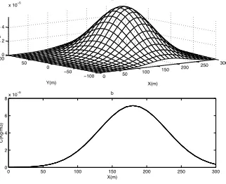
Figure 1: (a) Concentration distribution on the ground (b) Concentration distribution on the ground directly downwind of the release (onY = 0)

which is to be solved subject to the initial and boundary conditions (5) and (6). The solution of (7) can be derived using Laplace and Fourier transforms and is:

C = Q

8π32(K_xK_yK_z) 1 2_t32

e−

(X−U t)2 4Kxt −

Y2

4Ky t

×

e−(Z4−Kz tH)2 +e−

(Z+H)2 4Kz t

. (8)

Equation (8) is similar to the Gaussian model for an instantaneous point source [Seinfeld and Pandis, 1997]. Further, if we defineσ2

x=2Kxt,σy2=2Kytandσ2z=2Kzt, the two models are identical. Here

theσ’s are the standard deviations of the concentration distribution in theX,Y andZdirections. Therefore, there is a relation between the standard deviation of spread that arises in the Gaussian distribution and the eddy diffusivities in the advection-diffusion equation. The ground distribution of the concentration predicted using Equation (8) for the data valuesQ=1000 kg,Kx =Ky = 12

m2_s−1_,K

z= 0.2113m2s−1,t= 100sare shown in Figure 1. Figure 1(a) shows the concentration

distribution in theX−Y plane on the groundZ = 0, while Figure 1(b) shows the concentration distribution directly downwind (onY = 0), 100 seconds after the release.

4

Inverse Modelling

Inverse modelling is the extraction of model parameter information from data. It is a discipline that provides tools for the efficient use of data in the estimation of constants appearing in the mathematical models. In this inverse modelling problem, the structure of the equation is known; measurement of the outputs, time (t) and concentration (C), are available. Some of the parameters are unknown.

The aim of this section is to obtain the best or optimal estimate of the parameters (e.g, mass release Q, lateral eddy diffusivity Kx, source height H, distance of the source from measuring

point X, Y and time of the pollutant release relative to the measurement time) appearing in Equation (8) from measurements made at some position(s). The value ofKz can be found by

us-ing the theoretical modelKz=aZn [Yeh, 1975], and calculating a value at some reference height

(aand nare constants depend on atmospheric conditions.

f = ln

Q

4π32(K_x2K_z) 1 2

−3

2ln (T+t0)

−

X2

4Kx

+ Y

2

4Kx

+ H

2

4Kz

1

T+t0

−U2(₄T_K+t0)

x

+2U X 4Kx

(9)

wheref = ln(C),T+t0=t,t0is the (unknown) time after pollutant release when the measurement clock was started andT is the time (known) on that clock. It has also been assumed that lateral eddy diffusion in theX andY directions are equal,Ky =Kx. In simple terms, Equation (9) can be

written asf(T;b) whereT is the independent variable andb= [Q, H, X, Y, Kx, t0] is a parameter

vector.

4.1

Sensitivity Coefficients and Linear Dependence

Sensitivity coefficients are very important because they indicate the magnitude of change of the response f due to perturbations in the values of the parameters. They also provide information about which parameters can or cannot be estimated simultaneously. They are defined by the first derivatives off with respect to each parameter. The parameters can be simultaneously estimated without ambiguity if the sensitivity coefficients over the range of observations are not linearly dependent. Linear dependence occurs when the relation:

0 = α1∂fi

∂Q+α2

∂fi

∂H +α3

∂fi

∂Y +α4

∂fi

∂X

+α5 ∂fi

∂Kx

+α6∂fi ∂t0

for each of the observationsfi with not all αj equal to zero [Beck, 1977]. If we setα5 =α6 = 0

andα1,α2, α3,α4are certain non-zero constants, it can be showned that

α1∂fi

∂Q+α2

∂fi

∂H +α3

∂fi

∂Y +α4

∂fi

∂X = 0

This shows that the parameters in Equation (9) cannot be estimated simultaneously, i.e. pa-rameters cannot be estimated simultaneously if the data is collected at one location. Therefore measurements at more than one location are needed to estimate the parameters. Experimental results in Section 5.2 show that measurement locations cannot lie on a straight line on the ground to get good parameter estimates. Therefore concentration measurements taken from three differ-ent locations on the ground were considered to estimate the parameters in the air pollution model given by Equation (8).

Now consider an experiment in which data are generated at three different locations on the ground

P1 = (X0, Y0,0), P2 = (X0+x1, Y0+y1,0) and P3 = (X0+x2, Y0+y2,0). Therefore Equation

(9) will become:

f = ln

2Q

8π32(K_x2K_z) 1 2 −

3

2ln (T +t0)

−

(X0+x)2 4Kx

+(Y0+y)

2

4Kx

+ H

2

4Kz

1

T+t0

−U2(₄T_K+t0)

x

where (x, y) = (0,0), (x1, y1) or (x2, y2). This may be rearranged in the form:

f = β0+β1 x

T+t0

+β2 y

T+t0

+β3 1

T+t0

+β4

−

x2_+y2

4 (T+t0)+

U x

2 −

U2_(T+t

0)

4

−3

2ln (T+t0) (10)

where:

β0= ln

2Q

8π32(K_x2K_z) 1 2

+2U X0 4Kx

,

β1=−

X0

2Kx

, β2=−

Y0

2Kx

β3=

X2

0+Y02

4Kx

+ H

2

4Kz

, β4=

1

Kx

.

4.2

Computation of Parameters

The output of Equation (10) is a logarithm of pollution concentration as a function of time, space and a set of unknown parameters. On the other hand, pollution concentration measurements are available. The method, then, is to find estimates of the unknown parameters that best fit the measured data. Iff is the log of measured concentration and ˆf is the log of modelled concentration, the error in the fit of the measurement and the model,δ, is:

δ=

3n

i=1

fi−fˆi(b)

2

where 3nis the number of measurements and b= [β0, β1, β2, β3, β4, t0].

For the best match b must be varied to minimise δ. This result can be achieved using the Gauss-Newton method. Essentially, the procedure is iterative and requires good starting value estimates for all the parameters. If the starting values are not reasonably good, the iteration may not converge or may converge to a local minimum.

An alternative approach to this problem of parameter estimation is now considered. This is to transform both the data and the function so that there is a multiple linear relationship between the transformed data and transformed unknown coefficients within the minimisation iteration loop. This procedure requires a good starting value oft0 only. This can be calculated using the method

outlined later in this section. If the data values are transformed by letting:

W =f+3

2ln (T+t0), W1=

x

T+t0

, W2= y

T+t0

,

W3= 1

T+t0, andW4=−

x2+y2

4 (T+t0)

then the Equation 10 becomes:

The step then is to form estimates ofβ’s using multiple linear regression that best fit the measured valuesWi. If ˆWi are the modelled values, the errorδin the fit of measurements and the model is:

δ=

3n

i=1

(Wi−Wˆi)2 (12)

For the best matcht0 must be varied in the region [T0−, T0+] to minimiseδ. HereT0 is the

approximation of t0 and is an error. This minimisation result can be achieved using f min in

MATLAB. For the newt0valueβ0,β1,β2,β3andβ4can be calculated from Equation (11). Then,

by substituting these values into Equation (10), all the required parametersH, Q, X0, Y0 andKx

can be calculated.

4.3

Calculations of Initial Guess

t

Concentration distributions at the pointsP1 andP2can be written as:

CP1 =

2Q

8 (πt)32_(K2

xKz)

1 2

e−

(Xa−U t)2 4Kxt −

Y_a2

4Ky t−

H2

4Kz t ₍₁₃₎

CP2 =

2Q

8 (πt)32 _(K2

xKz)

1 2

e−

(Xb−U t)2 4Kxt −

Y_b2

4Ky t− H

2

4Kz t ₍₁₄₎

where t = t0 +T, Xa=X0, Xb=X0+x1, Ya=Y0, and Yb=Y0+y1. Dividing Equation (13) by

Equation (14) and then differentiating w.r.t. T followed by taking natural logarithms of both sides gives:

lnF+TF

F =−t0

F

F −

2x1

4Kx

where F = CP1

CP2

and F = dF_dT. The graph of lnF +T F_F plotted against F_F is a straight line, with a gradient of m = −t0 and intercept =− 2x1

4Kx (when T = 0). Note: The logarithms of

concentration distributions atP1 andP2have to be smoothed using polynomial fits for noisy data before applying the method.

5

Modelling Application

5.1

Source Term Estimation

To illustrate this inverse modelling application, consider an input of environmental data generated from an instantaneous point source of strength 1000 kg located at (0, 0, 20 m) in the Cartesian co-ordinate system. Figure 2 shows the concentration signal against time T at the pointsP1,P2

andP3, whereP1 = (5000,100,0), P2 = (5480,230,0) and P3= (5130,580,0), i.e. P1, P2 andP3

are on the vertices of a equilateral triangle of side 500m. For illustrative purposesKzand U are

taken as 0.211 and 1.80 respectively. The results of the source term estimation for the pollution concentration in Figure 2(a) are tabulated in Table 1. Then random relative noise of 1%, 2%, 3%, 4% and 5% were added to the simulated signal and the calculation of error in the source term was repeated for one hundred times for each case. Average error values of parameters are tabulated in rows 1 to 5 of Table 2.

5.2

Selection of Measurement Locations

0 100 200 300 400 500 600 700 0

0.5 1 1.5 2 2.5 3 3.5 4 4.5x 10

5

P1

P2

P3

Time(s)

C(Kg/m3)

a

0 100 200 300 400 500 600 700

0 0.5 1 1.5 2 2.5 3 3.5 4 4.5x 10

5

P1

P2

P3

C(Kg/m3)

b

Time(s)

Figure 2: (a) Concentration signal at the pointsP1,P2 and P3 on the ground with no noise, (b)

Concentration signal at the pointsP1,P2andP3 on the ground with noise of 5%.

Table 1. Source term estimates

t0 Kx X0 Y0 Q H

0.72 12 5000 100 1000 20

Table 2. Percentage errors in calculated parameters of the source term, for various relative noise levels.

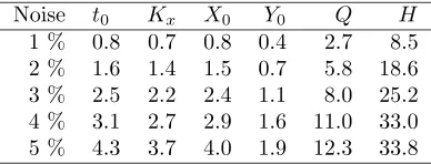
Noise t0 Kx X0 Y0 Q H

1 % 0.8 0.7 0.8 0.4 2.7 8.5 2 % 1.6 1.4 1.5 0.7 5.8 18.6 3 % 2.5 2.2 2.4 1.1 8.0 25.2 4 % 3.1 2.7 2.9 1.6 11.0 33.0 5 % 4.3 3.7 4.0 1.9 12.3 33.8

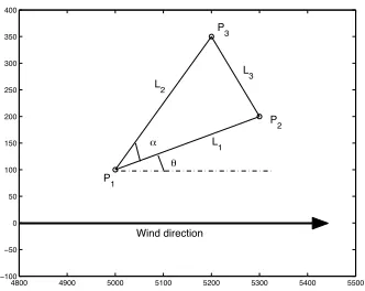
(i) All three stationsP1,P2andP3 lie on a straight line. (In Figure 4,P3 is on the lineP1P2.)

(ii) StationsP1,P2 andP3are on the vertices of a perpendicular isoscles triangle. (In Figure 4,

α= 90◦and L1=L2.)

(iii) P1, P2, and P3 are on the vertices of an equilateral triangle. (In figure 4, α = 60◦ and

L1=L2.)

In the first case whatever the values of θ, L1, L2 and L3, the calculated parameter values were

wrong even in the case of perfect simulated data. The error in parameter estimatesQandX0 of

the other two cases are plotted against the distance between the points in Figures 3(a) and 3(b) respectively. In each case, parameter values were calculated when the angle (θ) betweenP1P2and

0 100 200 300 400 500 600 700 800 900 1000 0

5 10 15 20 25 30 35

a b c

d

e

f

Distance between points

Error of Q in %

a− Case 2, θ=0 b− case 2, θ=15 c− case 2, θ=30 d− Case 3, θ=0 e− Case 3, θ=15 f− Case 3, θ=30

(m) a

0 100 200 300 400 500 600 700 800 900 1000

0 10 20 30 40 50 60 70 80 90

Error of X in %

Distance between points a

b

c

d e f

a− Case 2, θ=0 b− Case 2, θ=15 c− Case 2, θ=30 d− Case 3, θ=0 e− Case 3, θ=15 f− Case 3, θ=30

(m) b

Figure 3: (a) Error inQVs distance between points, (b) Error inX0 Vs distance between points.

4800 4900 5000 5100 5200 5300 5400 5500

−100

−50 0 50 100 150 200 250 300 350 400

Wind direction

θ α

L 2

L 3

L₁ P 3

P 2

P 1

6

Summary and Discussion

The goal of the work presented here was to develop an inverse model capable of simultaneously estimating the parameters appearing in the air pollution model for an instantaneous point source. The approach taken was to develop the inverse model as a non-linear least squares estimation problem in which the source term was estimated using pollution concentration measurements on the ground. The statistical basis of the least square inverse model allows for quantifying the un-certainty of the parameter estimates, which in turn allows for quantifying the unun-certainty of the simulation model predictions.

First in the process, it has been demonstrated that data from at least three spatial locations are needed to reliably estimate the parameters in the model. Secondly, we formulated the inverse model as a least squares minimization problem, and then we tested the methodology using artificial data generated from the forward problem.

The accuracy of the calculated parameter values varies with the distance between the measurement locations. Therefore the optimal design of the locations for pollution measurement on the ground is important. This is one possibility for improvement of the model.

This paper is a report of an initial study using both linear and nonlinear least squares estima-tion techniques for calculating source term parameters from an inverse model. The next phase of this study is to find estimates of source terms of pollution from steady and non-steady point sources of unknown time duration.

7

References

Beck, V.J., and Arnold, J.K, Parameter Estimation in Engineering and Science. John Wiley and Sons, New York, 1977.

Edwards, L.L., Freis, R.P., Peters L.G., and Gudiksen P.H., The use of non-linear regression anal-ysis for integrating pollutant concentration measurements with atmospheric dispersion modelling for source term estimation,Nuclear Technology, 101, 168–181, 1993.

Huang, C.H., Theory of dispersion in turbulent shear flow,Atmospheric Environment, 13, 453–463, 1979.

Kibler, J.F., and Suttles, J.T., Air pollution model parameter estimation using simulated LIDAR data,AIAA Journal, 15(10), 1381–1384, 1977.

Mulholland, M., and Seinfeld, J.H., Inverse air pollution modelling of urban scale carbon monoxide emissions,Atmospheric Environment, 29(4), 497–516, 1995.

Seinfeld, J.H., and Pandis, S.P.,Atmospheric chemistry and physics: from air pollution to climate change. John Wiley and Sons, New York, 1998.

Sohier, A., Rojas-Palma, C., and Liu, X., Towards a monitoring framework for the source term esti-mation during the early phase of an accidental release at nuclear power plant,Radiation protection dosimetry, 73(1–4), 231–234, 1997.