Smoothed particle simulation
of gravity waves in a
multi-fluid system
Songdong ShaoMSc, PhD, FHEA
Senior Lecturer in Environmental Fluid Mechanics, School of Engineering, Design and Technology, University of Bradford, UK
The generation and propagation of gravity waves in a multi-fluid system have significant environmental impacts. This paper presents an incompressible smoothed particle hydrodynamics model to simulate this process. The method is a mesh-free particle modelling approach that can treat the free surfaces and multi-interfaces in a straightforward manner. The proposed model is based on the general multi-fluid flow equations and uses a unified pressure formulation to address the interactions among the different components of the fluids. The model will be used to investigate the gravity currents generated from one fluid intruding into other fluids with different densities. The general features of the gravity current have been disclosed and the computed gravity wave height and wave propagation speed agree well with the theoretical analysis. The error analysis proved the convergence of the numerical scheme and it was found that the multi-fluid model is close to first-order accurate.
Notation
a wave amplitude generated by gravity current c solitary wave celerity
D depth of lock fluids d water depth
fls interaction force vector among different fluids
g gravitational acceleration vector g9 effective gravity
h smoothing distance
k empirical coefficient for current head velocity m particle mass
P pressure
r position vector
r* intermediate position vector
˜t time increment
u velocity vector
˜u velocity increment in prediction step
˜u velocity increment in correction step vh current head velocity
W interpolation kernel
˜X particle spacing
å relative error in wave amplitude ç solitary wave surface elevation ì dynamic viscosity of laminar flow
r fluid density
r0 averaged density of current head
r0 initial constant density r intermediate density
˜rB density difference between bottom and upper fluids
Subscripts
a reference particle b neighbouring particle l liquid component
m different fluids component s solid component
t time
x horizontal coordinate y vertical coordinate
1. Introduction
given a full summary on the experimental and numerical ap-proaches in this area.
The smoothed particle hydrodynamics (SPH) method is one highly robust particle modelling technique that was originally developed for astrophysical flows (Monaghan, 1992) and has since been modified for many kinds of incompressible free surface flows. Based on the weakly compressible SPH (WCSPH) algorithm, in which the fluid was treated as being slightly compressible, a variety of multi-fluid SPH models have been developed, such as for the dust gas flows (Monaghan and Kocharyan, 1995), gravity currents (Monaghanet al., 1999) and interfacial flows (Colagrossi and Landrini, 2003). The incompres-sible SPH (ISPH) modelling approach was developed based on the classic WCSPH but uses a strict hydrodynamic formulation to compute the fluid pressures (Shao and Lo, 2003). The subsequent research into ISPH models found that the computational effi-ciency and the pressure stability have improved in the ISPH algorithm (Ataie-Ashtiani and Shobeyri, 2008; Leeet al., 2008). Thus the ISPH model is selected as a promising tool to study the gravity current waves in this paper. The original single-fluid ISPH algorithm will be further developed based on the universal multi-fluid flow equations and the complicated interactions among the different fluid components will be simply treated by a unified pressure equation. The proposed model will be applied to a lock fluid flowing down a ramp into the two different fluids based on the work of Monaghanet al.(1999).
2. Development of multi-fluid ISPH model
2.1 Governing equations
The fluid ISPH model is established on the general multi-phase flow equations in the Lagrangian form. The continuity and momentum equations are written as below
1 rl
drl
dt þ=ul¼0
1 rs
drs
dt þ=us¼0
9 > > > = > > > ;
1:
rldul
dt ¼ =Plþrlgþìl= 2u
lþfls
rsdus
dt ¼ =Psþrsgþìs= 2u
sfls
9 > > > = > > > ;
2:
in which r is density; t represents time; u is velocity; P is pressure; g denotes gravitational acceleration; ì is dynamic viscosity and fls represents interaction forces among the
differ-ent fluid compondiffer-ents. The subscripts l and s refer to the different fluid components, or liquid and solid phases in a general term.
2.2 Solution methods
The ISPH solution methods employ a two-step prediction/correc-tion approach to solve the governing Equaprediction/correc-tions 1 and 2. The final flow velocity is calculated by using a time-marching procedure as
um,tþ1¼um,tþ˜um,tþ˜um,t (m¼l, s)
3:
in which˜um,tis velocity increment in the prediction step;˜um,t represents velocity increment in the correction step;um,tdenotes velocity at time t and um,tþ1 represents velocity at time tþ1:
Here m¼l, s refer to the different fluids.
The prediction step in the ISPH solutions is an explicit integra-tion in the time without enforcing the incompressibility. In this step, only the gravitational and viscous forces in Equation 2 are used and an intermediate particle velocity and position of the multi-fluid flows are obtained
˜ul,t ¼ ìl rl=
2u l
t
˜tþg˜t
˜us,t¼ ìs rs=
2u s
t
˜tþg˜t
9 > > > > = > > > > ;
4:
um,t¼um,tþ˜um,t
rm,t¼rm,tþum,t˜t 9 =
; (m¼l, s)
5:
in which ˜t is time increment; rmt denotes particle position at timetandrm,trepresents intermediate particle position.
After the predictive computations, the incompressibility of the fluid system is not satisfied. This is manifested by the fact that the intermediate density of the fluid particlesrdeviate from the initial constant densityr0:Thus the densities of the particles are
required to be corrected to the initial values in the correction step to satisfy the incompressibility.
The velocity increment in the correction step is calculated by
rl˜ul,t ¼ =Ptþ1˜t
rs˜us,t ¼ =Ptþ1˜t
9 = ;
6:
momentum Equations 1 and 2 and represented for each of the fluid components as
= 1
rm=Ptþ1
¼r
0r
r0(˜t)2 (m¼1, s)
7:
Finally, the spatial position of the fluid particles is calculated by using a central scheme in time as:
rm,tþ1¼rm,tþ
um,tþum,tþ1
ð Þ
2 ˜t (m¼1, s)
8:
in whichrm,tþ1is position of the particle at timetþ1:
2.3 SPH theories and formulations
In an SPH framework, the modelled fluid media are discretised as an assembly of a large number of individual particles. The particle interaction zone is supposed to be around each particle. All of the terms in the governing Equations 1 and 2 are described as the interactions between the reference particle and its neighbours. Thus the computational grid is not required. Combined with the adequate initial and boundary conditions, a particular hydrody-namic problem can be solved exclusively through the particle properties. The SPH numerical scheme is free from the numerical diffusions since the advection term is calculated by the motion of the particles. Besides, the deformation of the free surfaces and multi-interfaces can easily be tracked by the particles.
In the SPH formulations, the motion of each particle is calculated through the interactions with its neighbouring particles using an analytical kernel function. The detailed reviews of the SPH principles are provided by Monaghan (1992). Among a variety of the kernels documented in the literature, the spline-based kernel normalised in two dimensions is widely used in different hydro-dynamic calculations. The following standard SPH formulations are used in the proposed multi-fluid ISPH model.
The densityraof a fluid particleais calculated by
ra¼X b
mbW(jrarbj,h)
9:
in which a and b are reference particle and its neighbours; mb represents particle mass; ra and rb are particle positions; W is interpolation kernel and h denotes smoothing distance, which determines the range of the particle interactions.
The pressure gradient uses the following form as
1 r=P
a
¼X
b mb
Pa r2 a
þPb
r2 b
=aWab
10:
in which the summation is over all the particles other than particle aand =aWab represents the gradient of the kernel taken with respect to the position of particlea:
The Laplacian for the pressure term and the laminar viscosity are formulated as a hybrid of a standard SPH first derivative com-bined with a finite difference approximation for the first deriva-tive. The purpose is to eliminate the numerical instability caused by the particle disorders arising from the second derivative of the SPH kernel (Shao and Lo, 2003). They are represented in the following symmetrical forms to conserve the particle properties
= 1
r=P
a
¼ X
b mb
8 (raþrb)2
3(PaPb)(rarb)=aWab rarb
j j2
11:
ì r=
2u
a
¼ X
b mb
2ìa=raþìb=rb raþrb
3(uaub)(rarb)=aWab rarb
j j2
12:
3. Boundary conditions, free surfaces and multi-interfaces
3.1 Impermeable solid walls
In the ISPH numerical scheme, the solid walls are modelled by the fixed wall particles that balance the pressures of the inner fluid particles and prevent them from penetrating the wall. The pressure Poisson Equation 7 is solved on these wall particles. When an inner fluid particle approaches the wall, the pressure of the wall particles increases, and vice versa. For details, see Shao and Lo (2003).
3.2 Free surfaces and multi-interfaces
The free surfaces can be easily and accurately tracked by using the fluid particles. As there is no fluid particle existing in the outer region of the free surface, the particle density on the free surface should drop significantly. This criterion is used to judge the surface particles and a zero pressure is given to each of the surface particles when solving the pressure Poisson Equation 7.
a lighter fluid and a heavier fluid, this particle is then recognised as an interface particle. It is obvious that the ISPH model can also describe the multi-interfaces in a straightforward manner without involving the complicated front-tracking algorithms that are commonly used in a grid method.
4. Model validation
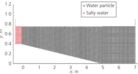
The proposed multi-fluid ISPH model is first validated by a discontinuous density current flowing down a sloping bed based on the experimental and numerical work of Canteroet al.(2003). The numerical settings of the flume geometry and two different fluids are shown in Figure 1. The salty water with a density of 1007 kg/m3 is released to the ambient water with a density of
1000 kg/m3 over a slope of 0.08. In the ISPH computations, a
shorter computational domain of 7.0 m is used to save the central processing unit (CPU) time. The initial particle spacing is chosen as˜X¼0.01 m and thus the total computational particles include 43 050 water particles and 1336 salty water particles. In Cantero
et al.(2003), this problem was solved by using the RANS model with a discontinuity front capturing technique based on a finite-element solver and the computations were compared with the experiment performed by Professor Marcelo H. Garcia (Cantero
et al., 2003).
To validate the ISPH modelling accuracy, the computed time-dependent leading edge of the density current front is compared with the experimental data and computational fluid dynamics (CFD) results of Canteroet al.(2003) in Figure 2. It shows that the general agreement among the three data sets is satisfactory. The CFD results overpredict the experimental leading edge before time t¼50 s but underpredict it after t¼75 s. In contrast, the ISPH computations underpredict the experiment at the beginning of the computation but are more close to the experiment at the later stage of the density current flow. The maximum error between the ISPH results and the experimental data is 6.2%, while it is 11.7% for the CFD simulations of Cantero et al.
(2003). Here it should be mentioned that Cantero et al. (2003) used a mesh system with 45 676 nodes and 45 000 bilinear quadrilateral elements to reproduce the experiment that has a similar spatial accuracy as the ISPH particle resolutions.
5. Model application – gravity current flowing down a ramp into stratified fluids
5.1 Numerical tank settings
Many of the gravity currents that happen in a practical field involve the flows into a density-stratified fluid field. The interface of the stratified fluids can have several effects on the gravity current, such as diverting the flow and initiating a large amplitude solitary wave that can have harmful influences over a long distance (Monaghanet al., 1999).
To investigate a practical situation, we now consider a mild ramp with 208 slope, consisting of the lock region, horizontal section and ramp. The lock fluids have a density of 1210 kg/m3and the
lower tank fluids have a density of 1070 kg/m3overlaid by a fresh
water layer with a density of 1000 kg/m3: According to the
numerical settings of Monaghanet al.(1999), the lock region has a length of 0.5 m and depth of 0.25 m. To reduce the computa-tional cost, the left end of the tank was set 0.75 m from the bottom of the ramp. The bottom fluid layer has a depth of 0.23 m. The proposed multi-fluid ISPH model aims to reproduce the numerical results from the established WCSPH approach of Monaghan et al. (1999) and further investigate the velocity structures near the interface during the different fluid interactions. The initial set-up of the numerical tank for the ramp flow is shown in Figure 3.
In the ISPH computations, an initial particle spacing of
˜X¼0.01 m is used by balancing the computational efficiency and accuracy. There are a total of 13 000 particles involved, consisting of the lock particles, light particles and heavy particles, as shown in Figure 3. Different types of fluid particles are given different identifiers and thus the free surfaces and interfaces 0
0·2 0·4 0·6 0·8 1·0 1·2
0 1 2 3 4 5 6 7
y
: m
x: m
[image:4.595.321.547.136.313.2]Water particle Salty water
Figure 1.Numerical tank set-up with two different fluids based on Canteroet al.(2003)
0 2 4 6 8
0 20 40 60 80 100
Leading edge: m
Time: s
Exp
[image:4.595.60.295.630.756.2]CFD ISPH
between the different fluids can be identified throughout the computations.
5.2 Model verifications
The computed particle snapshots during the gravity current flowing down the ramp after the release are shown in Figures 4(a)–(c) at three different times, matching the WCSPH computa-tions of Monaghanet al.(1999). The simulated flow patterns are very similar to those shown in Figure 18 in Monaghan et al.
(1999). There is a qualitatively good agreement between the two different SPH modelling approaches, and the proposed multi-fluid ISPH model can well predict the overturning of the gravity current head and the subsequent intruding and mixing processes.
The ISPH results predicted an averaged velocity of the gravity current head at 0.38 m/s. An analytical value of 0.43 m/s can be calculated by using Britter and Linden (1980)
vh, k(g9D)1=2
13:
in which D is the depth of the lock fluids, g9¼g˜r=r is the effective gravity andkis an empirical coefficient in Monaghanet al.(1999).
Besides, from Figure 4 the wave amplitude generated by the descending gravity current is computed to be 0.22 m. By using the pressure balance analysis, Monaghan et al. (1999) gave an estimation of the wave amplitude at
a ¼r0v2h=˜rBg
14:
in which˜rB is the density difference between the bottom fluids and the fresh water andr0 is the averaged density of the gravity current head. This formula gives a value of 0.23 m that is quite close to the ISPH computations with an error of 4.3%.
To further validate the accuracy of the ISPH computations, the analytical solitary wave profiles based on the Boussinesq equation
(Lee et al., 1982) have also been provided in the figures for comparison. It shows that the generated solitary waves computed by the ISPH agree satisfactorily with the theoretical solutions, with slight under-predictions at the wave crest. The analytical solitary wave profile is calculated from Leeet al.(1982)
ç(x,t)¼asech2
ffiffiffiffiffiffiffiffi 3a 4d3
s
(xct) 2
4
3 5
15:
in which ç is wave surface elevation, d represents water depth andc¼pffiffiffiffiffiffiffiffiffiffiffiffiffiffiffiffiffiffiffiffig(dþa)is the solitary wave celerity.
Here it needs to be pointed out that the left-hand side (LHS) 0
0·2 0·4 0·6 0·8 1·0
⫺0·8 ⫺0·4 0 0·4 0·8 1·2 1·6
y
: m
x: m
[image:5.595.301.538.133.548.2]Light particle Heavy particle Lock particle
Figure 3.Initial set-up of numerical tank for gravity flow, with three different fluids
0 0·2 0·4 0·6 0·8 1·0
⫺0·6 ⫺0·4 ⫺0·2 0 0·2 0·4 0·6
y
: m
x: m (a)
Light particle Heavy particle Lock particle
0 0·2 0·4 0·6 0·8 1·0
⫺0·6 ⫺0·4 ⫺0·2 0 0·2 0·4 0·6
y
: m
x: m (b)
Light particle Heavy particle Lock particle
0 0·2 0·4 0·6 0·8 1·0
⫺0·6 ⫺0·4 ⫺0·2 0 0·2 0·4 0·6
y
: m
x: m (c)
Light particle Heavy particle Lock particle
[image:5.595.42.276.134.264.2]boundary is a solid boundary that is fully reflective. The ISPH computations were stopped before the generated wave reached the LHS boundary and thus the simulated waves were not influenced by the existence of the wall.
5.3 Analysis of flow features
The computed particle snapshots in Figure 4 show that when the gravity current descends the ramp and interacts with the interface of the bottom fluids and the upper fresh water, then substantial wrapping and overturning processes occur. The current head is the main site of the intensive mixing, with the fresh water moving around and behind the head, mixing with the lock fluids. The ISPH simulations have disclosed many of the features found in the physical experiment and the numerical simulations of Mon-aghanet al.(1999). Owing to the continuous entrainment of the fresh water as the descending gravity current intrudes, the gravity current contains distinct regions mixed with the lower–higher density fluids. For example, some pockets of the fresh water are enclosed inside the lock fluid region. The gravity current has raised the interface between the bottom fluids and the fresh water by forcing the fluids in front of it to move up and around the head, generating a solitary wave. However, it should be pointed out that one difference between the ISPH and WCSPH (Mon-aghanet al., 1999) computations is that the WCSPH predicted a plug-like gravity current head (Figure 18 in Monaghan et al., 1999), while the ISPH predicted a boundary-fitted gravity current head. This is because Monaghan et al. (1999) used a repulsive boundary treatment while the ISPH used a hydrodynamic bound-ary with the Neumann conditions enforced (Shao and Lo, 2003).
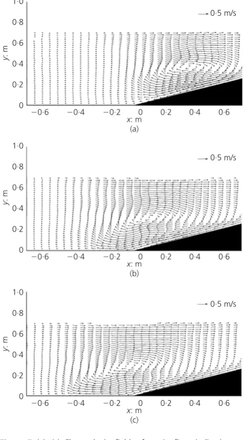
Further examining the flow velocity fields in Figures 5(a)–(c), it is shown that there exists a strong flow circulation zone near the gravity current front. Owing to the sudden release of the lock fluids, the gravity current is generated and a counter-current of the fresh water flows into the lock region, producing a velocity circulation and carrying it forward as the gravity current descends the ramp. Meanwhile, the range and amplitude of the flow circulations continue to increase and the influence zones spread to the fluids further away. The ISPH simulations have disclosed a strong flow circulation over the current front and a nearly constant velocity region in the current head, which is consistent with the field and experimental observations.
The computed pressure fields of the gravity current flow at time
t¼5.7 s are shown in Figure 6. For analysis, the interface profile of the gravity current is also shown. The figure indicates that the computed pressure fields are quite stable and there is no pressure noise near the interfaces, which is an indication that the ISPH pressure solution scheme is sound. It has also been found that the pressure contours are nearly evenly spaced within the ambient fluids and the gravity current body and the amplitude of the pressure is consistent with the current profile. That is to say, the pressure is higher inside the gravity flows that provide the momentum to move the fluid forward. This implies that the pressure distributions in a gravity current flow can be treated as a hydrostatic problem,
0 0·2 0·4 0·6 0·8 1·0
⫺0·6 ⫺0·4 ⫺0·2 0 0·2 0·4 0·6
y
: m
x: m (a)
0·5 m/s
0 0·2 0·4 0·6 0·8 1·0
⫺0·6 ⫺0·4 ⫺0·2 0 0·2 0·4 0·6
y
: m
x: m (b)
0·5 m/s
0 0·2 0·4 0·6 0·8 1·0
⫺0·6 ⫺0·4 ⫺0·2 0 0·2 0·4 0·6
y
: m
x: m (c)
[image:6.595.315.554.141.571.2]0·5 m/s
Figure 5.(a)–(c). Flow velocity fields of gravity flow, indicating flow circulations near current head: (a)t¼3.4 s; (b)t¼4.2 s; (c)t¼4.7 s
0 0·2 0·4 0·6 0·8 1·0
⫺0·6 ⫺0·4 ⫺0·2 0 0·2 0·4 0·6
y
: m
x: m
Gravity current front
0·8 0·7 0·6 0·5 0·4 0·3 0·2 0·1 0·0
p g/ρ
[image:6.595.317.555.635.756.2]providing a good rationale that most numerical models based on the shallow water equations (SWE) can simulate the gravity current quite well in practice (Looseet al., 2005; Younget al., 2005).
5.4 Numerical error analysis
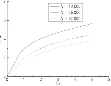
To analyse the convergence behaviour of the numerical algorithm, additional computations with two different particle spacings˜X
have been made and the particle numbers used are N¼26 000 and 52 000, respectively. The generated solitary wave is used for the analysis. The errors are calculated as the difference between the numerically generated wave amplitude and the theoretical value by using the formulation in Xuet al.(2009) as
å¼ a
numaanalytical
aanalytical 3100%
16:
The time-dependent errors in the wave amplitude computed by using the original and the additional two ISPH particle resolu-tions are shown in Figure 7. It clearly shows that as the particle numbers increase, that is, as the particle sizes decrease, the errors decrease rapidly indicating the convergence of the numerical scheme. The maximum errors found in the wave amplitude happen at the end of the simulations when the particle disorder is the highest. The error is 5.7% for the roughest simulation and 3.8% for the finest simulation, respectively. A simple error analysis (Shao and Lo, 2003) showed that the spatial accuracy of the multi-fluid ISPH model is close to but slightly below first-order accurate. This is less satisfactory than a single-fluid ISPH numerical scheme and more robust treatment of the interfaces would be able to further improve the spatial accuracy.
6. Conclusions
A multi-fluid ISPH model has been developed to simulate the interactions of the fluids with different densities. The model has
been validated against the case of the salty water intruding into the ambient fluids and applied to a gravity current flowing down a ramp into different fluid layers. The ISPH computations were found to be in good agreement with the documented data. The computed solitary wave celerity and wave height are consistent with the analytical results. The computed velocity fields disclose the distinct flow circulations, and the overturning and wrapping of the fluids can be naturally captured by the particle modelling approach. The computed pressure fields suggest that the pressure distributions under a gravity flow are essentially hydrostatic and thus the numerical models based on the SWE should work well for similar applications. Although further quantitative validation is required, the proposed modelling approach could provide a promising trend that is worth exploring. All of the computations were carried out on a DELL Precision T7500 with dual CPUs 3.20 G Hz and RAM 48.0 G.
Also it should be noted that the latest research by Xu et al.
(2009) indicated that by only imposing the density invariance in ISPH such as in Shao and Lo (2003) could lead to relatively large errors where the flow Reynolds number is high. This was not found in the tested cases in this paper and it could be partly attributed to the relatively smaller flow Reynolds num-ber. More robust validations should be carried out in future to address the solver stability under a wider range of testing conditions.
Acknowledgements
This research work is supported by the Royal Society research grant 2008/R2 RG080561. The manuscript was finalised when the author was visiting Nanyang Technological University, Singa-pore under a Tan Chin Tuan Exchange Fellowship.
REFERENCES
Ataie-Ashtiani B and Shobeyri G(2008) Numerical simulation of landslide impulsive waves by incompressible smoothed particle hydrodynamics.International Journal for Numerical Methods in Fluids56(2): 209–232.
Britter RE and Linden PF(1980) The motion of the front of a gravity current travelling down an incline.Journal of Fluid Mechanics99(3): 531–543.
Cantero MI, Garcı´a MH, Buscaglia GC, Bombardelli FA and Dari EA(2003) Multidimensional CFD simulation of a
discontinuous density current. InProceedings of 30th IAHR Congress, Water Engineering and Research in a Learning Society, Thessaloniki(Ganoulis J and Prinos P (eds)). pp. 405–411.
Colagrossi A and Landrini M(2003) Numerical simulation of interfacial flows by smoothed particle hydrodynamics.
Journal of Computational Physics191(2): 448–475.
Firoozabadi B, Farhanieh B and Rad M(2003) Hydrodynamics of two-dimensional, laminar turbid density currents.Journal of Hydraulic Research41(6): 623–630.
Gotoh H and Sakai T(2006) Key issues in the particle method for 0
2 4 6 8
0 1 2 3 4 5 6
ε
: %
t: s
N⫽13 000
N⫽26 000
[image:7.595.48.276.581.757.2]N⫽52 000
computation of wave breaking.Coastal Engineering53(2–3): 171–179.
Imran J, Kassem A and Khan SM(2004) Three-dimensional modeling of density current. Part I: flow in straight confined and unconfined channels.Journal of Hydraulic Research 42(6): 578–590.
Lee ES, Moulinec C, Xu R,et al.(2008) Comparisons of weakly compressible and truly incompressible algorithms for the SPH mesh free particle method.Journal of Computational Physics227(18): 8417–8436.
Lee JJ, Skjelbreia JE and Raichlen F(1982) Measurement of velocities in solitary waves.Journal of Waterways, Port, Coastal and Ocean Division, ASCE108(WW2): 200–218. Loose B, Nino CY and Escauriaza MC(2005) Finite volume
modeling of variable density shallow-water flow equations for a well-mixed estuary: Application to the Rı´o Maipo estuary in central Chile.Journal of Hydraulic Research43(4): 339– 350.
Monaghan JJ(1992) Smoothed particle hydrodynamics.Annual Review of Astronomy and Astrophysics30: 543–574. Monaghan JJ(2007) Gravity current interaction with interfaces.
Annual Review of Fluid Mechanics39: 245–261.
Monaghan JJ, Cas RAF, Kos AM and Hallworth M(1999) Gravity
currents descending a ramp in a stratified tank.Journal of Fluid Mechanics379: 39–69.
Monaghan JJ and Kocharyan A(1995) SPH simulation of multi-phase flow.Computer Physics Communications87(1–2): 225–235.
Patterson MD, Simpson JE, Dalziel SB and Nikiforakis N(2005) Numerical modelling of two-dimensional and axisymmetric gravity currents.International Journal for Numerical Methods in Fluids47(10–11): 1221–1227.
Rottman JW and Simpson JE(1983) Gravity currents produced by instantaneous releases of a heavy fluid in a rectangular channel.Journal of Fluid Mechanics135: 95–110. Shao SD and Lo EYM(2003) Incompressible SPH method for
simulating Newtonian and non-Newtonian flows with a free surface.Advances in Water Resources26(7): 787–800. Xu R, Stansby P and Laurence D(2009) Accuracy and stability in
incompressible SPH (ISPH) based on the projection method and a new approach.Journal of Computational Physics 228(18): 6703–6725.
Young DL, Lin QH and Murugesan K(2005) Two-dimensional simulation of a thermally stratified reservoir with high sediment-laden inflow.Journal of Hydraulic Research43(4): 351–365.
WHAT DO YOU THINK?
To discuss this paper, please email up to 500 words to the editor at [email protected]. Your contribution will be forwarded to the author(s) for a reply and, if considered appropriate by the editorial panel, will be published as a discussion in a future issue of the journal.