ABSTRACT
Context.The massive infrared dark cloud G0.253+0.016 projected∼45 pc from the Galactic centre contains∼105 M
of dense gas
whilst being mostly devoid of observed star-formation tracers.
Aims.Our goals are therefore to scrutinise the physical properties, dynamics and structure of this cloud with reference to its star-forming potential.
Methods.We have carried out a concerted SMA and IRAM 30 m study of this enigmatic cloud in dust continuum, CO isotopologues, several shock tracing molecules, as well as H2CO to trace the gas temperature. In addition, we include ancillary far-IR and sub-mm Herscheland SCUBA data in our analysis.
Results.We detect and characterise a total of 36 dust cores within G0.253+0.016 at 1.3 mm and 1.37 mm, with masses between 25 and approximately 250M, and find that the kinetic temperature of the gas traced by H2CO ratios is>320 K on size-scales of∼0.15 pc.
Analysis of the position–velocity diagrams of our observed lines shows broad linewidths and strong shock emission in the south of the cloud, indicating that G0.253+0.016 is colliding with another cloud atvLSR ∼70 km s−1. We confirm via an analysis of the observed
dynamics in the Central Molecular Zone that it is an elongated structure, orientated with Sgr B2 closer to the Sun than Sgr A*, however our results suggest that the actual geometry may be more complex than an elliptical ring. We find that the column density probability distribution function of G0.253+0.016 derived from SMA and SCUBA dust continuum emission is log-normal with no discernible power-law tail, consistent with little star formation, and that its width can be explained in the framework of theory predicting the density structure of clouds created by supersonic, magnetised turbulence. We also present theΔ-variance spectrum of this region, a proxy for the density power spectrum of the cloud, and show it is consistent with that expected for clouds with no current star formation. Finally, we show that even after determining a scaled column density threshold for star formation by incorporating the effects of the increased turbulence in the cloud, we would still expect ten stars with masses>15Mto form in G0.253+0.016. If these cannot be accounted for by new radio continuum observations, then further physical aspects may be important, such as the background column density level, which would turn an absolute column density threshold for star formation into a critical over-density.
Conclusions.We conclude that G0.253+0.016 contains high-temperatures and wide-spread shocks, displaying evidence of interaction with a nearby cloud which we identify atvLSR∼70 km s−1. Our analysis of the structure of the cloud can be well-explained by theory
of magnetised turbulence, and is consistent with little or no current star formation. Using G0.253+0.016 as a test-bed of the conditions required for star formation in a different physical environment to that of nearby clouds, we also conclude that there is not one column density threshold for star formation, but instead this value is dependant on the local physical conditions.
Key words.stars: formation – ISM: clouds – dust, extinction – ISM: kinematics and dynamics – ISM: structure – Galaxy: center
1. Introduction
Determining how massive clusters (103−105M
) form has a pro-found effect on how we interpret observations of star formation in external galaxies. As the majority of stars form in clusters (Lada & Lada 2003;de Wit et al. 2005), and because massive clusters yield – either via statistics or by virtue of their phys-ical conditions – the most massive stars, these clusters are the engines which produce the objects that dominate the luminosity of galaxies. Therefore, uncovering how and where these mas-sive clusters can form is of central importance in understanding how galaxies evolve, and may provide hints as to how cluster formation proceeds at all masses.
FITS files of data corresponding to Figs. 2, 4, 10, 11 are only
available at the CDS via anonymous ftp to cdsarc.u-strasbg.fr (130.79.128.5) or via
http://cdsarc.u-strasbg.fr/viz-bin/qcat?J/A+A/568/A56
To understand the conditions that lead to cluster formation, it is necessary to observe the structure of the gas and dust, as well as kinematics, of a cluster forming cloud before star forma-tion processes begin blurring the initial condiforma-tions. Observing the formation of massive clusters within our own Galaxy has the obvious advantage of resolving clouds that typically fall within a single resolution element for observations of distant galaxies.
One of the most exceptional candidates for a massive clus-ter progenitor is the cloud G0.253+0.016 near the Galactic cen-tre (e.g.,Lis et al. 1994;Lis & Menten 1998;Longmore et al. 2012). The global dust properties of G0.253+0.016 (also known as M0.25+0.01) have been shown by previous authors (e.g.Lis et al. 1994; Lis & Menten 1998; Lis et al. 2001; Longmore et al. 2012;Immer et al. 2012) to be cold (∼18–27 K), dense (n∼7.3×10⁴–6×105cm−3) and massive (M=1.3–7×10⁵M
).
However, minimal evidence has been found for ongoing star for-mation. The H2O maser and 8.4 GHz radio continuum
obser-vations ofLis et al.(1994) uncovered a single H2O maser near
Table 1.Summary of observed/imaged lines.
Facility Line or continuum Frequency Angular resolution Imaged spectral Sensitivity
(GHz) (arcsec) resolution (km s−1) (mJy beam−1)
SMA SiO (5–4) 217.105 4.4×2.9, PA 0.7◦ 2, 5 68, 48
SMA H2CO 3(0, 3)–2(0, 2) 218.222 4.3×2.9, PA – 1.0◦ 2, 5 70, 50
SMA CH3OH 4(2, 2)–3(1, 2)-E 218.440 4.3×2.9, PA – 1.1◦ 2, 5 76, 56
SMA H2CO 3(2, 2)–2(2, 1) 218.476a
SMA H2CO 3(2, 1)–2(2, 0) 218.760 4.3×2.9, PA – 1.0◦ 2, 5 65, 43
SMA C18O (2–1) 219.560 4.3×2.9, PA 1.0◦ 2, 5 74, 54
SMA HNCO 10(0, 10)–9(0, 9) 219.798 4.3×2.9, PA 0.7◦ 2, 5 67, 46
SMA SO 6(5)–5(4) 219.949 4.3×2.9, PA 1.0◦ 2, 5 68, 47
SMA 13CO (2–1) 220.399 4.2×2.9, PA 0.7◦ 2, 5 240, 220
SMA CH3OH 8(–1, 8)–7(0, 7)-E 229.759 4.3×2.7, PA 3.6◦ 2, 5 74, 51
SMA 12CO (2–1) 230.538 4.3×2.7, PA 4.4◦ 2, 5 890, 890
SMA 4 GHz continuum 216.9–220.9 4.3×2.9, PA – 1.1◦ 2.5
SMA 4 GHz continuum 228.9–232.9 4.3×2.7, PA 4.0◦ 2.5
IRAM 30 m 13CO (2–1) 220.399 11.8 2, 5 2500, 1600
IRAM 30 m 12CO (2–1) 230.538 11.2 2, 5 6000, 5000
SMA+IRAM 30 m 13CO (2–1) 220.399 4.2×2.9, PA 0.7◦ 2, 5 200, 140
SMA+IRAM 30 m 12CO (2-1) 230.538 4.3×2.7, PA 4.4◦ 2, 5 500, 500
Notes.(a)Blended with CH
3OH 4(2, 2)- 3(1, 2)-E .
the 350μm continuum peak position, but no coincident radio emission.SpitzerandHerschelobservations have also confirmed that no protostars are seen in the cloud in the mid- or far-IR up to 70μm (e.g.,Longmore et al. 2012).Rodríguez & Zapata (2013) presented Very Large Array (VLA) 1.3 and 5.6 cm ra-dio continuum observations of G0.253+0.016 which detected three compact radio sources towards the eastern edge of the cloud, which have thermal spectral indices and correspond to B0.5 stars. These could be signposts of massive star formation in G0.253+0.016; however, as will be discussed below, they do not correspond to dense cores of gas traced by mm emission.
It is interesting to note that the similarly massive cloud Sgr B2, which is not far away from G0.253+0.016, actively forms stars and is one of the most prominent sites of star for-mation in the Galaxy. Therefore, how can such a massive and dense molecular cloud as G0.253+0.016 currently not be form-ing stars? A possible explanation for the high star-formation activity in Sgr B2 is that one of the dust lanes associated with the Galactic bar intersects with the x2 orbits of the gas in the
Central Molecular Zone (CMZ) at the position of Sgr B2, and thus we would expect an elevated level of star formation at this position. Yet this does not straightforwardly explain the compar-atively lesser degree of star formation towards the other point of intersection with the dust lanes of the bar on the opposite side of the CMZ, Sgr C (e.g.,Kendrew et al. 2013). One possible explanation could involve an asymmetry in the material falling inwards along the two dust lanes of the bar, or in the gas orbit-ing the CMZ, providorbit-ing less material for collision at the posi-tion of Sgr C. Alternatively, the star formaposi-tion in Sgr B2 could be enhanced by its recent passage close to the Galaxy’s central black hole, Sgr A* (Longmore et al. 2013). Of course, the ob-served differences between Sgr B2 and Sgr C may be due to a combination of these effects.
Recently, G0.253+0.016 has also been studied using MALT90 and APEX observations (Rathborne et al. 2014), and ALMA SO observations have shown evidence for a cloud-cloud collision with G0.253+0.016 (Higuchi et al. 2014). In fact, such cloud-cloud collisions may provide a way to collect enough dense gas to produce massive clusters (e.g.,Fukui et al. 2014).
With reference to these possible scenarios, in this work we aim to determine the current state of star formation in
G0.253+0.016, as well as its star-forming fate (i.e., whether it will form a star cluster), by investigating the structure of the cloud, its internal dynamics, its interaction with the CMZ environment and its local stability to collapse.
Section2outlines our 1.3 mm Submillimeter Array (SMA) and Institut de Radioastronomie Millimétrique (IRAM) 30 m observations, as well as ancillary far-IR and sub-mmHerschel and Submillimeter Common User Bolometer Array (SCUBA; Holland et al. 1999) data. Section3presents our observational results from the continuum and line observations, including the column density probability distribution function (PDF) of G0.253+0.016, and determination of temperatures from H2CO.
Section 4 presents our discussion, which covers the topics of the internal dynamics of G0.253+0.016, the interaction of G0.253+0.016 with its environment, as well as its current star-formation activity and potential. Our conclusions are given in Sect.5.
2. Observations and archival data
2.1. SMA line and continuum observations
Observations of G0.253+0.016 were conducted on 9 June 2012 with the SMA in its compact array configuration under good weather conditions (the optical depth at 225 GHz was be-low 0.1). The two 4 GHz sidebands were placed at 218.9 and 230.9 GHz (1.37 and 1.30 mm), with each of the 48 SMA cor-relator chunks per sideband having 128 channels and a spec-tral resolution of 0.812 MHz or 1.1 km s−1. Seven of the eight SMA antennas were available for the observation, providing baseline lengths between 16.4 m and 77.0 m and thus a largest angular scale of approximately 20–21. Table 1 lists the ob-served lines and continuum, their frequencies, synthesised beam sizes and the rms noise in the final images. The observations consisted of a 6-pointing mosaic covering G0.253+0.016, with spacing between pointings of approximately half the primary-beam width (54–58). The total time on-source was 4.5 h. The gain, bandpass and flux calibrators were 1733–130, 3C 279 and Titan. Data reduction was carried out using the MIR package1, followed by imaging in MIRIAD (Sault et al. 1995).
1 The MIR package and cookbook can be found athttps://www.
upper 3 ×80 of the map, decreasing the sensitivity in this area by√2. The total time on-source was 77.5 min. Spectra and maps were made using the GILDAS package. When averaging over the entire map, all lines detected in the SMA observations were detected with the IRAM 30 m. In addition, several weak uniden-tified lines at 217.823, 219.875, 229.900 and 229.931 GHz were also detected in the average spectrum over the map. The12CO
and13CO line emission had sufficient signal-to-noise to create
maps and to be combined with the SMA line channel maps. The combination was carried out using the feather task in CASA. The beam size and rms noise for the12CO and 13CO uncom-bined IRAM 30 m and comuncom-bined SMA+IRAM 30 m maps are given in Table1.
2.3. Herschel far-IR and SCUBA 450μm data
We also made use of archival data from theHerschelsatellite (Pilbratt et al. 2010). Photometric data at 70, 160, 250, 350 and 500 μm were obtained with the PACS (Poglitsch et al. 2010) and SPIRE (Griffin et al. 2010) bolometric cameras on September 7, 2010 (operational day 481) as part of the Hi-Gal survey of the Galactic plane (Molinari et al. 2010). These obser-vations were performed in parallel-mode (PACS and SPIRE in tandem) with a fast scan rate of 60s−1, and the data set used
(obsids 1342204102, 1342204103) covers a 2◦×2◦patch of the Galactic plane in two perpendicular scan directions, centred on the Galactic coordinates [0.0, 0.0] and including G0.253+0.016. For PACS, we downloaded the relevant Level 1 data from the HerschelScience Archive (Leon et al. 2009), which were pro-duced by the HCSS 10.3.0 bulk reprocessing of the raw data. We used the HIPE software (track 12.0, build 2491Ott 2010) to apply an additional correction of the bolometer response, based on the drift of the evaporator temperature (Balog et al. 2014) before using the SCANAMORPHOS software (Roussel 2013), version 22.0, for further drift corrections, 1/fnoise removal, and final mapping. For SPIRE, we downloaded the Level 2 data (cal-ibrated for extended emission) from the HCSS 10.3.0 bulk re-processing and combined the two scan directions with the HIPE mosaic task. The pixel sizes for the PACS and SPIRE data, listed by increasing wavelength, are 3.2, 3.2, 6, 10 and 14and the as-sumed FWHM beam sizes are 8.8, 13.0, 23.3, 30.3 and 42.4. The PACS 70 and 160μm beam was derived from 2D Gaussian fits to point sources in the image, and the SPIRE beams were as-sumed to be the geometric mean of the values stated in Table2 ofTraficante et al.(2011). We refrained from using the convolu-tion kernels published byAniano et al.(2011) since they are not adapted to the specifics of the parallel-mode PSFs.
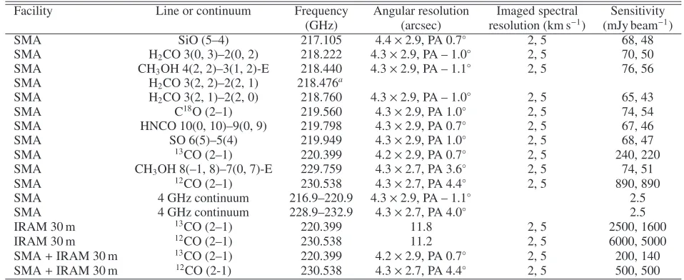
SPIRE images. Firstly, all the threeHerschelimages at shorter wavelengths were convolved to a resolution of 42.4, and re-projected to the same FITS header using Montage (Jacob et al. 2009). The large-scale background was then removed from each image using the algorithm based on that outlined inBattersby et al.(2011), which we now describe. When creating the model of the background emission, we smoothed each image by 20 and used this image directly instead of fitting Gaussians in lat-itude to the emission. A source mask was created by masking emission above 3σin a difference image created by subtracting the smoothed 500μm image from the original 500μm image. This process was repeated, using the mask derived in the previ-ous iteration until the 3σlevel of the masked difference image converged. This source mask was applied to each image before it was smoothed to determine the background to be subtracted. When fitting the modified blackbodies, we applied temperature andβ(the opacity power-law index) dependent colour correc-tions to the PACS 100μm model images2. We did not apply any colour corrections to the SPIRE models as these were small: less than 4% for temperatures between 15 and 40 K (Griffin et al. 2013). The results of the fit included: the flux scaling of the fit, which essentially gives the column density, and the temperature at each point in the image. We produced three model images by evaluating the model at 450μm when assuming three fixed val-ues ofβ: 1.5, 1.75 and 2.0. Figure1presents the temperature map and model 450μm image forβ = 1.75. The derivedβ = 1.75 temperature map is in good agreement (<10%) with the map presented byLongmore et al. (2012); the temperatures across G0.253+0.016 range from∼19 to∼30 K. There is a remaining background contribution from the CMZ after large-scale back-ground subtraction in the temperature map presented here and inLongmore et al.(2012), which will slightly increase the mea-sured temperature of the cloud. If a higher threshold than 3σ was used to create the background mask, over-subtraction of the source occurred at the edges of the cloud, leading to incor-rect temperature and flux values at these positions. Therefore we opted to increase the size of the mask to 3σ to obtain correct relative values of temperature and flux across G0.253+0.016, while noting that the absolute temperature may be overestimated at most by 10% or 3 K within the region covered by our SMA observations.
After the model 450 μm image was produced, the SCUBA 450μm image was convolved to the same resolution (42.4), using a similar method to that ofAniano et al.(2011). 2 Section 4.3 of http://herschel.esac.esa.int/twiki/pub/
Table 2.Measured and calculated properties of the cores detected in SMA continuum, exclusive of the combination with the short-spacing SCUBA emission presented in Sect.3.2.
Core Lower side band Upper side band
number Peak position Speak Sint Mass Column density Diameter Peak position Speak Sint Mass Column density Diameter 24.8 GHz
(J2000) (mJy beam−1) (mJy) (M
) (g cm−2) (pc)b (J2000) (mJy beam−1) (mJy) (M
) (g cm−2) (pc)b emissionc
1 17:46:06.1 –28:41:41.1 23.1 63.2 119 0.39 0.35 17:46:06.2 –28:41:40.6 26.3 101.7 151 0.37 0.41 N 2 17:46:06.9 –28:41:32.6 22.7 60.9 123 0.41 0.36 17:46:06.9 –28:41:32.6 20.9 24.6 39 0.32 0.22 N 3 17:46:07.1 –28:41:46.1 13.5 37.2 74 0.24 0.33 17:46:07.1 –28:41:45.6 12.8 44.3 69 0.19 0.38 N 4 17:46:07.3 –28:42:04.6 22.5 50.9 95 0.37 0.29 17:46:07.3 –28:42:03.1 25.7 76.3 112 0.36 0.37 Y 5 17:46:07.5 –28:43:56.6 28.3 29.1 44 0.38 0.19 17:46:07.5 –28:43:58.1 36.8 158.7 185 0.41 0.51 N 6 17:46:07.9 –28:42:19.6 22.1 25.6 47 0.36 0.21 17:46:07.9 –28:42:20.6 21.4 40.8 57 0.29 0.32 N 7 17:46:08.3 –28:41:44.1 18.6 125.6 252 0.33 0.53 17:46:08.4 –28:41:45.6 22.6 98.8 155 0.34 0.45 N 8 17:46:08.6 –28:43:45.6 14.1 30.4 52 0.21 0.29 17:46:08.2 –28:43:50.1 18.8 78.7 101 0.23 0.50 Y 9 17:46:08.6 –28:42:09.1 31.6 111.1 216 0.55 0.38 17:46:08.7 –28:42:10.1 30.3 110.5 169 0.44 0.39 Y 10 17:46:09.1 –28:43:18.6 14.9 53.2 96 0.24 0.45 17:46:09.3 –28:43:17.1 16.0 66.4 94 0.22 0.49 Y 11 17:46:09.5 –28:42:07.1 26.5 61.8 122 0.47 0.29 17:46:09.5 –28:42:06.6 33.9 74.9 115 0.50 0.31 N 12 17:46:09.7 –28:43:32.1 13.2 13.4 25 0.22 0.19 17:46:09.6 –28:43:30.6 15.5 33.0 47 0.21 0.30 Y 13 17:46:10.1 –28:42:44.6 21.0 77.0 151 0.37 0.37 17:46:10.1 –28:42:46.1 22.1 60.2 92 0.32 0.32 Y 14 17:46:10.3 –28:43:40.6 14.8 39.0 70 0.24 0.32 17:46:10.4 –28:43:39.6 15.1 21.5 30 0.20 0.24 N 15 17:46:10.3 –28:42:28.1 28.4 109.9 219 0.51 0.39 17:46:10.3 –28:42:28.1 25.4 93.1 146 0.38 0.39 Y 16 17:46:10.6 –28:42:36.1 25.0 33.9 67 0.44 0.23 17:46:10.6 –28:42:36.1 22.3 30.9 48 0.33 0.23 Y 17 17:46:10.6 –28:43:08.1 12.6 78.8 150 0.21 0.54 17:46:10.9 –28:42:58.6 16.0 72.2 109 0.23 0.46 Y 18 17:46:10.6 –28:42:17.6 51.7 78.4 156 0.92 0.31 17:46:10.6 –28:42:17.6 58.7 118.7 185 0.87 0.39 Y 19 17:46:11.2 –28:43:33.1 30.8 102.5 181 0.48 0.40 17:46:10.7 –28:43:31.6 15.9 42.0 59 0.22 0.32 Y 20 17:46:11.2 –28:43:13.6 17.2 61.8 114 0.28 0.41 17:46:11.2 –28:43:09.1 14.7 63.2 92 0.20 0.42 Y
21 17:46:08.0 –28:43:13.6 20.8 30.3 48 0.29 0.29 Y
22a 17:46:08.1 –28:43:50.6 18.3 38.9 63 0.27 0.27 Y
23 17:46:08.4 –28:41:33.6 16.8 45.6 92 0.30 0.32 N
24 17:46:09.3 –28:42:26.1 19.8 25.9 50 0.34 0.22 Y
25a 17:46:10.7 –28:43:29.6 14.3 14.3 26 0.23 U Y
26a 17:46:11.2 –28:42:19.6 27.4 43.0 84 0.48 0.26 Y
27 17:46:11.4 –28:42:14.1 20.6 28.8 55 0.35 0.22 N
28 17:46:12.0 –28:42:56.6 18.8 30.4 54 0.30 0.30 Y
29a 17:46:07.4 –28:41:34.6 18.7 31.2 50 0.29 0.26 N
30 17:46:07.7 –28:41:09.1 28.7 107.2 159 0.41 0.44 N
31 17:46:08.6 –28:41:16.6 22.9 22.9 34 0.33 U Y
32a 17:46:09.1 –28:41:49.6 13.0 19.5 30 0.19 0.23 N
33 17:46:09.6 –28:44:01.6 26.4 86.4 113 0.33 0.44 N
34 17:46:10.4 –28:41:56.1 18.2 52.7 77 0.25 0.39 N
35a 17:46:11.4 –28:42:19.6 23.9 23.9 36 0.34 U N
36 17:46:11.9 –28:43:31.6 28.8 33.5 44 0.36 0.23 Y
Notes.(a)Core 22 is associated with cores 5 and 8. Core 25 is associated with core 19. Core 26 is associated with core 18. Core 27 is partially
associated with core 35. Core 29 is associated with core 2. Core 32 is associated with core 7. Core 35 is partially associated with core 27.
(b)Geometric mean diameter of the core. U denotes that the core is unresolved.(c)Y denotes that the core is associated with 25 GHz emission
[image:4.595.40.375.539.681.2]above 0.125 mJy beam−1in a 2.2×1.9beam (Mills et al., in prep.).
Fig. 1. Left: temperature map derived from SED fits to Herschel images assuming β = 1.75. Right: model 450 μm image de-rived from Herschel data, assuming β = 1.75. Contours are 50, 100, 150 and 200, 250 and 300 Jy beam−1. Greyscale: –35 to
350 Jy beam−1. The beam (FWHM 42.4) is
shown in the bottom left corner.
This consisted of taking the inverse transform of the ratio of Fourier transforms of the SPIRE 500μm and SCUBA beams. We made a model of the SCUBA 450 μm beam using the parameters of the first two components of the beam given in Table2ofHogerheijde & Sandell(2000), consisting of an 8 FWHM inner beam and a 30 first error beam with relative
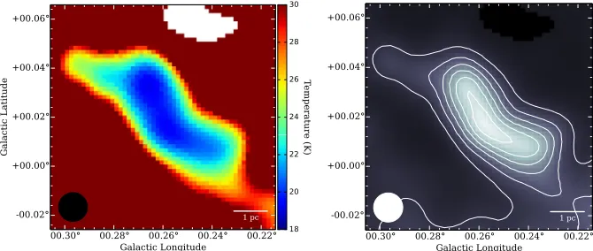
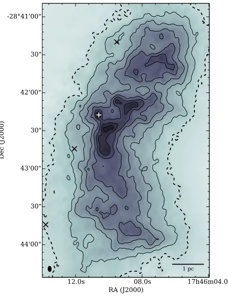
Fig. 2.Left panel: map of the 218.9 GHz or 1.37 mm continuum emission observed with the SMA. Contours are –5, 5, 6, 8, 10, 12, 16 and 20× rms noise=2.5 mJy beam−1. Greyscale: –2 to 50 mJy beam−1. The synthesised beam is shown in the bottom left corner: 4.3×2.9, PA=–1.1◦. Right panel: map of the 230.9 GHz or 1.30 mm continuum emission observed with the SMA. The contours and stretch are the same as in the left panel. The synthesised beam is shown in the bottom left corner: 4.3×2.7, PA=4.0◦. Inboth panelsthe plus sign marks the position of the water maser reported byLis et al.(1994) and the crosses mark (from north to south, respectively) the positions of the 1.3 cm sources VLA 4 to 6 from Rodríguez & Zapata(2013).
[6.053, 5.619, 4.993] Jy beam−1 and [0.65, 0.62, 0.59]
respec-tively forβ = [1.5, 1.75, 2.0]. Thus the calibration factor of the original SCUBA 450μm image to theHerschelcalibration is 0.62±0.03, with the error determined from the range in as-sumed values ofβ.
As combining the two SMA sideband continuum images did not significantly increase the continuum sensitivity and would not straightforwardly represent one frequency, we decided to combine the SMA 1.3 mm upper sideband continuum image with the single dish SCUBA image. To do this we scaled our calibrated SCUBA 450 μm image to 1.3 mm, by eval-uating the model of the emission derived from the Herschel data at 1.3 mm and finding the pixel-to-pixel ratio between the 450μm and 1.3 mm model images. We used this ratio im-age to then scale the flux calibrated SCUBA 450 μm image to 1.3 mm. This resulted in three images at 1.3 mm, one for each of the assumed values ofβ. These three images were then combined with the SMA 1.3 mm image using the feather task in CASA.
3. Results
3.1. SMA continuum emission
The two panels of Fig.2 show respectively the lower and up-per sideband continuum observed with only the SMA, centred at 230.9 and 218.9 GHz, or 1.30 and 1.37 mm. The position of the maser observed byLis et al. (1994) is marked as a plus sign, and the three crosses mark the positions of the 20.9 GHz or 1.3 cm sources VLA 4 to 6 fromRodríguez & Zapata(2013). The maser coincides with the brightest 1 mm continuum source in the region, however no obvious dust emission is associ-ated with theRodríguez & Zapata(2013) 1.3 cm sources. The
brightest 1 mm continuum source detected in our observations is also the same as the 1.1 mm source detected byKauffmann et al.(2013) at 280 GHz, however further cloud structure is also apparent above 5σin our 1.30 and 1.37 mm maps.
To characterise the continuum emission detected at 1.30 and 1.37 mm, we produced dendrograms (e.g.Rosolowsky et al. 2008;Goodman et al. 2009) using theastrodendro software3. We chose the flux limit above which fluxes were measured to be 2σ; the required peak flux of the leaves of the dendrogram, i.e. the highest density structures which had no further structures embedded within them, to be at least 5σ; and the required flux difference between embedded structuresΔFto beσ. The astro-dendrocode was run separately on both the 1.37 and 1.30 mm (lower and upper side bands, respectively) continuum images. The leaves are listed in Table2, where we refer to them as cores. Confirmed cores which were detected in both images and had an overlap in pixels greater than 30 pixels are given first, listing the core number, peak position, peak fluxSpeak, integrated fluxSint,
massM, peak column densityNpeakand geometric mean
diam-eter Dfor the 1.37 and 1.30 mm images (or lower and upper sidebands), respectively.
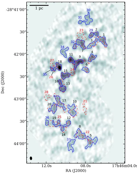
Fig. 3.Map of the cores detected in 218.9 and 230.9 GHz (1.37 mm and 1.30 mm) continuum emission observed with the SMA, in red dashed and blue solid contours, respectively. The 1.30 mm continuum emission is shown in greyscale, ranging between –2.5 and 40 mJy beam−1. The
cores are numbered as listed in Table2. The synthesised beam is shown in the bottom left corner: 4.3×2.7, PA=4.0◦.
the images which has no intrinsic emission is boosted above 5σ by the noise is less than once for a million-pixel image (based on simulations of images with injected noise measured with the astrodendrosoftware). As there are 9.1×104pixels covered by the mosaic pattern in each continuum image, we would expect less than one false detection every ten images; given two images, there is thus a<20% chance that there is one false source in one of them. Therefore, it is likely that the majority, if not all, of the nine cores detected without a counterpart in the other continuum image are real. These nine cores consist of the 16 cores listed without a match in Table2, minus the seven cores which were partially associated with other cores (markedain the table).
The masses of the cores were determined using the equation,
M = gSintd
2
B(ν,T)κν (1)
wheregis the gas-to-dust ratio,dis the distance,B(ν,T) is the black body function, which is a function of frequencyν and temperatureT, andκν is the frequency-dependent opacity. We
assumed a distance of 8.4 ±0.6 kpc (Reid et al. 2009), and used the temperature maps derived from theHerscheldata in Sect.2.3to determine the temperature at the core positions. The gas-to-dust ratio for the solar neighbourhood was calculated to be 154, given the ratio between the mass of dust and mass of hydrogen of 0.0091 (Draine 2011). The gas-to-dust ratio in the Galactic centre is roughly half this value, due to a metallicity twice as high as the solar value (e.g.Najarro et al. 2009). Thus we assumed a gas-to-dust ratio for the Galactic centre of 77. We assumed an opacity of 0.701 cm2g−1 at 1.30 mm, taken
fromOssenkopf & Henning(1994) forn = 105cm−3 and thin
ice mantles. For the opacity at 1.37 mm, we fit a line in log space to the same opacities above wavelengths of 40μm, where the dependence of opacity on wavelength becomes a power law, and extrapolated the 1.3 mm opacity to 1.37 mm to ob-tain 0.602 cm2g−1. These opacities are uncertain by a factor of
two or less (Ossenkopf & Henning 1994) and thus dominate the overall mass uncertainty. The peak column densities were calcu-lated in the same fashion, instead using the peak fluxes and divid-ing by the relevant SMA beam area. The geometric mean diam-eter was calculated from the area covered by each dendrogram core structure.
Continuum observations carried out with the VLA at 24.1 to 36.4 GHz (1.2 to 0.8 cm) with∼2resolution display emission towards 20 of the detected 1.3 mm cores (Mills et al., in prep.). Those which are associated with 24.8 GHz or 1.2 cm emission above 0.125 mJy beam−1 in a 2.2 ×1.9 beam (Mills et al.,
in prep.) are marked with a Y in the final column of Table2. The brightest 1.2 cm continuum source that is coincident with a core (Core 9), has a peak flux density of 0.55 mJy beam−1at 1.2 cm and a flat spectral index, indicating optically thin free-free emis-sion. Core 9 has a peak flux of 30.3 mJy beam−1 at 1.3 mm,
therefore the extrapolated ionised gas emission should only con-tribute a few percent to the flux of this source at 1.3 mm. The most obvious coincidences of dust and 1.3 cm ionised gas emis-sion exist for Cores 9, 13 and 26 (also the edge of core 18). Thus these may be indicating the presence of high-mass star formation within G0.253+0.016.
3.2. Combined SMA and SCUBA single dish emission
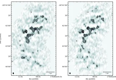
Figure 4 presents the combined SMA and scaled SCUBA 1.3 mm continuum emission derived as described in Sect.2.3. This is one of the few continuum maps that successfully com-bines the single-dish with interferometer data and hence recovers all spatial scales from the interferometer resolution limit to the scales covered by the bolometer. With this data we can now anal-yse the column density structure of this enigmatic cloud in great depth. Figure4shows that the three 1.3 cm sources discovered in Rodríguez & Zapata(2013) again appear to be coincident with the edge of the cloud and not any dense, and thus possibly star-forming, material within it. The brightest continuum emission lies between the declinations of –28◦42and –28◦43. Above a declination of –28◦42, there is also a somewhat separated is-land of 1.3 mm emission. There is comparatively less emission towards the south of the cloud.
To obtain an estimate of the cloud mass, the mass corre-sponding to each pixel in the combined 1.3 mm image was de-termined via the same method as described in Sect.3.1, taking into account the beam size. The total mass was then found by summing these values above the dashed black contour in Fig.4, corresponding to a column density of 2×1022cm−2forβ=1.75.
The mass values determined for the three values ofβwere 10, 9.1 and 7.9×10⁴ M
forβ = 1.5, 1.75 and 2.0, respectively.
Although sightly smaller, this range of values compares well with previous estimates of the cloud mass (M=1.3–7×10⁵M
,
Fig. 4.Map of the 230.9 GHz or 1.3 mm continuum emission observed with the SMA, combined with the scaled single-dish SCUBA 1.3 mm emission derived in Sect.2.3. Contours are –6, 6, 10, 14, 18, 22, 26 and 30×4 mJy beam−1. Greyscale: –20 to 150 mJy beam−1. The synthesised
beam is the same as the SMA-only image, and is shown in the bottom left corner: 4.3 ×2.7, PA=4.0◦. The plus sign marks the position of the water maser reported byLis et al.(1994) and the crosses mark (from north to south, respectively) the positions of the 1.3 cm sources VLA 4 to 6 fromRodríguez & Zapata(2013). The dashed black contour shows a column density of 2×1022cm−2forβ=1.75, used as the outer
boundary of the cloud when determining its total mass.
authors to determine both the total and dense gas mass (AK>0.1 and 0.8 mag respectively) correspond4 to 8.3×1020 cm−2 and 6.6×1021 cm−2, which are both lower than the lower H
2
col-umn density limit used to determine the mass of G0.253+0.016: 2×1022cm−2.
3.3. Column density probability distribution function (PDF) of G0.253+0.016
The PDF of the volume or column densities within molecular clouds has previously been used as a tool to investigate the ef-fect of various competing physical processes within them (e.g. Kainulainen et al. 2009; Schneider et al. 2013; Federrath & Klessen 2013). Often a range of densities within the PDF can be fit well by a log-normal distribution. This distribution of den-sities is thought to arise from a series of multiplicative, randomly distributed shocks in a turbulent medium, which result in a log-normal volume density distribution due to the central limit theo-rem (Vazquez-Semadeni 1994;Ballesteros-Paredes et al. 2011). When the detected cloud volume densities along the line of sight 4 To determine the column densities from A
K, we assumed AK =
1 mag is equivalent toAv = 8.8 mag (Kainulainen & Tan 2013) and N(H2)/Av=0.94×1021cm−2mag−1(Bohlin et al. 1978).
Fig. 5. Probability distribution functions (PDFs) of column density for G0.253+0.016, assuming three values of β when scaling the SCUBA 450μm emission: 1.5, 1.75 and 2.0 (red, black, and blue, re-spectively). The density-values in the PDF shown forβ=1.5 and 2.0 have been multiplied by factors of 0.87 and 1/0.87, respectively. The PDFs are derived from images with a resolution of 4.3 ×2.7, or 0.18×0.11 pc at a distance of 8.4 kpc. They-axis shows the number of pixelsNpixper logarithmic bin. The dashed line shows the column
density corresponding to the 3σnoise level for theβ = 1.75 image, assuming a temperature for the outer regions of the cloud of 30 K.
remain correlated, the column density should represent its mean along the line of sight, and thus will be correspondingly narrower but exhibit the same functional shape. The log-normal form of the column density PDF can be expressed as:
p(η) dη=p0(η) exp
−(η−μ)2/(2σ2η)
dη, (2)
whereη = ln (N/N ) with N being the column density;p0(η)
is the normalisation constant, which isp0(η)=1/
√
2πσηin the
case of a purely log-normal distribution;μis the mean value ofη andσηis the dispersion.
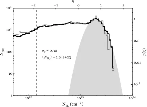
[image:7.595.308.555.80.266.2]Fig. 6.Probability distribution functions (PDFs) of the column den-sity for G0.253+0.016, assuming a value ofβ=1.75. The black line shows the PDF for the combined image (4.3 ×2.7 resolution, or 0.18 × 0.11 pc ford = 8.4 kpc), and the grey line the SCUBA-only PDF (8 or 0.33 pc resolution). The lefty-axis shows the number of pixels per logarithmic binNpix, and the righty-axis is the normalised
probabilityp(η). The topx-axis is displays the dimensionless parameter
η=ln (N/N ). The dashed line shows the column density correspond-ing to the 3σnoise level, assuming a temperature of 30 K. The Poisson errors are shown as error bars. The grey filled area corresponds to a by-eye fit to the combined PDF, giving the fit parametersση, describing the
PDF width, andNH2, the average density, whose values are shown in
the figure.
the 3σnoise level for theβ=1.75 image, assuming a temper-ature for the outer regions of the cloud of 30 K. Due to the fact the resultant shapes of PDFs using these three assumptions are very similar for different values ofβ(modulo the shift and thus error of±1513% in absolute value of the column density), we will continue our study using the images and PDF made under the assumptionβ=1.75.
The grey line in Fig.6 shows the column density PDF of G0.253+0.016 derived from the scaled SCUBA image, and the black line shows the PDF derived from the combined 1.3 mm image. In addition to showing the column density and number of pixels in each logarithmic bin on the bottom and leftx- and y-axes, we also show the equivalent values ofηandp(η) along the upper and right axes. Both PDFs have a similar shape at low densities: a plateau in the PDF with almost constant prob-ability below a column density of 1.4×1023 cm−2. Above this density, the PDFs resemble a log-normal function. Compared to the combined PDF, the SCUBA-only PDF peaks more promi-nently at the mean density, possibly due to beam-averaging. It also falls below the combined PDF at hydrogen column densi-ties of3×1023 cm−2, which is a further effect of resolution.
Similarly, the combined PDF appears to be also altered by the spatial resolution above∼4×1023cm−2, where it suffers a sud-den drop. This is supported by the fact that the sud-densest contin-uum core in G0.253+0.016, Core 18, is unresolved, with a col-umn density of 4.4×1023cm−2. Higher resolution observations
would thus “fill in” the PDF above this density.
Therefore, up to densities of 4×1023cm−2, our observations
show no evidence of a power-law tail in the column density PDF of G0.253+0.016, and therefore we find no indication that the process of collapse and consequent star formation is widespread within the cloud. Nevertheless, we can compare the properties of the log-normal portion of the combined PDF to those found for
other clouds, and to predictions from theory, which we discuss in Sect.4.3.
We also note that due to the distance of G0.253+0.016, in-tervening clouds may change its observed PDF, for instance by acting to narrow its true width (Schneider et al. 2014). However, as we utilised SCUBA observations to determine the lower den-sities in our PDF, which remove diffuse emission more extended than 4, emission from diffuse foreground and background dust should not strongly affect the observed PDF.
3.4. SMA line emission
Figure7presents the observed SMA spectra for both sidebands on a short baseline (antennas 1 and 7), averaged over the six observed mosaic fields. The detected lines are marked and are listed in Table1. Although their frequencies lie within the ob-served bands, both the dense and hot gas tracers13CS(5–4) and
the k ladder of CH3CN(12–11) were not detected. The detected
lines fall into three groups: shock tracers: methanol, SiO, HNCO and SO; CO isotopologues as diffuse gas tracers:12CO, 13CO and C18O; and H
2CO lines as temperature probes.
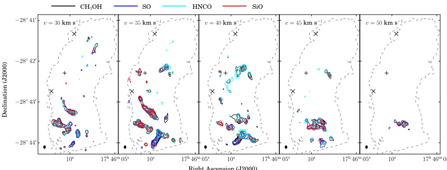
Figure8presents the channel maps of the shock tracing lines. This includes the brightest observed methanol line, CH3OH
4(2, 2)–3(1, 2)-E at 218.44 GHz (the other methanol lines ob-served also present emission similar to that seen in Fig.8), as well as SiO, HNCO and SO. In all transitions, the morphology is similar with the emission being brightest towards the south-ern half of G0.253+0.016. This is also seen for the H2CO and
the CO isotopologue emission. In addition, a similar morphol-ogy is seen in collisionally excited methanol masers at 36 GHz (Mills et al. 2014, Mills et al. in prep.). In Fig.8, three spoke-like filaments can be seen, which are most prominent in the 30 and 35 km s−1channels, radiating out from an apex lying at
ap-proximately 17h46m08s –28◦4336 (J2000). In the 45 km s−1
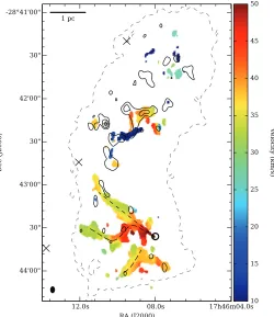
channel, the dominant emission moves westward towards the apex and becomes ring-like. In the 50 km s−1channel it becomes more compact and continues to move towards the apex point. This behaviour suggests a large velocity gradient (spanning at least 20 km s−1) along these filaments. Figure9presents the first
moment map of the 4(2, 2)–3(1, 2)-E methanol line confirming this, where we have marked the three filaments with dashed lines. In Sect.4.1we discuss the possible mechanisms to pro-duce such a velocity gradient. In Fig.9, the 1.3 mm SMA dust continuum emission is also shown in black contours. Although they do not directly line-up with one another, there is an appar-ent spatial correlation between the methanol and dust continuum emission.
Figure10compares the 1.3 mm dust continuum cores and line emission integrated from 0 to 60 km s−1 for several lines. The line emission is that observed with the SMA, apart from
13CO which also incorporates the IRAM 30 m emission, which
will be described further in the following section. The bright-est 1.3 mm source (Core 18) is not obviously detected in any of the integrated images, although it lies just above 5σin C18O
in the 40 km s−1channel. Otherwise, there is line emission
con-sistently offset to the east of core 18 (e.g. in H2CO where the
emission is coincident with Core 26). Other examples of co-incident emission are CH3OH, SiO, HNCO and H2CO
associ-ated with Cores 4, 6 and 24, and CH3OH, SiO and HNCO with
[image:8.595.42.290.81.263.2]Fig. 7.Observed SMA spectra of both sidebands, averaged over the six observed fields for a short baseline (antennas 1 and 7).
−28◦44
−28◦43
−28◦42
−28◦41
17h46m05s
10s 10s 17h46m05s 10s 17h46m05s 10s 17h46m05s 10s 17h46m05s
Right Ascension (J2000)
De
cl
in
at
io
n
(J2000)
[image:9.595.66.522.292.466.2]CH3OH SO HNCO SiO
Fig. 8.SMA CH3OH 4(2, 2)–3(1, 2)-E, SO, HNCO and SiO emission. Contours are –5, 5, 8, 12, 16 and 20×the rms noise values for each line
given in Table1, for a spectral resolution of 5 km s−1. A synthesised beam of 4.3×2.9, PA=0◦is shown in the bottom left corner. The plus
sign marks the position of the water maser reported byLis et al.(1994) and the crosses mark (from north to south, respectively) the positions of the 1.3 cm sources VLA 4 and 5 fromRodríguez & Zapata(2013). The dashed grey contour shows the combined dust continuum emission at a level of 0.024 mJy beam−1, the lowest solid black contour shown in Fig.4.
the morphology of the line and dust continuum emission, al-though not all dust cores have a distinct counterpart in the line emission.
3.5. Combined SMA and IRAM 30 m emission
Figure11presents the combined SMA and IRAM 30 m 13CO emission observed towards G0.253+0.016, imaged in 5 km s−1
channels. The emission from G0.253+0.016 extends between approximately –10 to 55 km s−1. In addition, there is another
cloud which can be seen between 60 and 85 km s−1, which
covers the south-east half of the map. We will refer to this as the 70 km s−1 cloud. There is a large velocity gradient across
G0.253+0.016, from blueshifted in the north to redshifted in the south, which has been previously noted byLis & Menten(1998) andRathborne et al.(2014). Between 15 and 35 km s−1, and most obvious in the 30 and 35 km s−1channels, there is a cavity in the 13CO emission in the north half of the cloud, which is seen at
ap-proximately 17h46m09s.5 –28◦4230(J2000). This hole or
cav-ity may be due to optical depth effects, as the combined 1.3 mm continuum shows the brightest emission and thus densest ma-terial close to this position. The morphology of G0.253+0.016
also appears curved, with its sections of emission connecting to form a semi-circular bow directed to the east. The emission can also be seen to curve in a similar manner in the SMA contin-uum and line emission in Fig.10. Between 40 and 50 km s−1, the bar of emission in the south of the cloud has a velocity gradi-ent which increases to the west, similarly to the gradigradi-ent seen in the lines presented in Figs.8and9. Between 50 and 85 km s−1,
the morphology of the 13CO emission connects smoothly to
the 70 km s−1 cloud, where it first contracts to a small area of
emission in the south of the cloud in the 55 km s−1channel, and
then expands from the same point into the diagonal bar of emis-sion which can be seen in the 65 and 70 km s−1channels.
Figure 12 displays combined SMA plus IRAM 30 mm
13CO spectra at three selected positions in the cloud, which are
marked with crosses of the same colour in Fig. 11. The po-sitions are (ordered by increasing declination): 17h46m10.5s – 28◦4335.5 (blue dotted line), 17h46m08.0s -28◦4210.7 (red
dashed line), and 17h46m09.6s–28◦4143.5 (orange solid line,
all J2000). Although the three spectra are broad and offset in ve-locity, they all display a relatively narrow peak at 41.8, 30.6 and 34.6 km s−1, respectively. Fitting the brightest components of the
Fig. 9. First moment map of the 4(2, 2)–3(1, 2)-E methanol line at 218.440 GHz. Black contours show the 230.9 GHz or 1.30 mm con-tinuum emission observed with the SMA at 5, 10 and 20× rms noise=2.5 mJy beam−1. The synthesised beam for the methanol line
is shown in the bottom left corner: 4.3×2.9, PA=–1.1◦. The plus sign marks the position of the water maser reported byLis et al.(1994) and the crosses mark (from north to south, respectively) the positions of the 1.3 cm sources VLA 4 to 6 fromRodríguez & Zapata(2013). The thick black circle in the south of the image marks the position of point A and the dashed lines show the positions of the three filaments mentioned in the text. The dashed grey contour shows the combined dust contin-uum emission at a level of 0.024 mJy beam−1, the lowest black contour
shown in Fig.4.
of this narrower component to be 13.9, 11.4 and 14.1 km s−1. In
addition to the bright (relatively) narrow components, there is also non-Gaussian emission which extends to lower velocities. Emission from the 70 km s−1 cloud can be seen to varying
de-grees in each spectrum.
Figure 13 presents a position velocity (PV) diagram col-lapsed along the Right Ascension axis of the cube for 13CO
in greyscale and grey contours, overplotted with CH3OH
trac-ing shocks in yellow contours. We chose CH3OH as it was
the brightest shock-tracing molecule, however SiO also shows a similar morphology in PV space. Both G0.253+0.016 and the 70 km s−1cloud can be clearly seen in 13CO emission. The
methanol emission is only seen towards G0.253+0.016 and not the cloud at 70 km s−1. As previously noted, the shock-tracing
emission is concentrated towards the south of G0.253+0.016, and spans the largest velocity range in this region: from∼25 to 55 km s−1 at a declination of –28◦4333(J2000). The shock
emission at this declination also reaches out along a bridge of
13CO emission to the 70 km s−1 cloud. The peak of the 13CO
emission lies between 30 and 45 km s−1, behind the velocity
of the arrowhead of methanol emission pointing into the other cloud. We discuss the possibility that these features are evi-dence of a collision between G0.253+0.016 and the 70 km s−1
cloud in Sect.4.1. At higher declinations, there are two velocity
components: one at∼10 and one at∼40 km s−1. By comparison with Figs.9and10, we can see that the 10 km s−1component is
associated with Cores 15 and 24, and the 40 km s−1component
with Core 9. Whilst these two methanol velocity components with associated dust cores are very close on the sky, they are separated by 30 km s−1. Thus although they lie within the
con-fines of the larger G0.253+0.016 cloud traced by 13CO, there
is evidence for strong dynamics in the north of the cloud. It is also interesting to note that the13CO emission peaks at a
veloc-ity of∼25 km s−1, lying in between these two methanol velocity components.
3.6. Kinetic temperatures from H2CO
The ratio of the integrated fluxes of H2CO lines can be used
to determine the kinetic temperature of the gas (e.g.Mangum & Wootten 1993). For example, recent single-dish observations of the CMZ using H2CO line ratios have determined average
temperatures of ∼65 K (Ao et al. 2013). These gas tures are significantly higher than the measured dust tempera-tures in the CMZ (e.g. 21±2 K,Pierce-Price et al. 2000) and in G0.253+0.016 (<30 K from Sect.2.3). The cause of these diff er-ent dust and gas temperatures may be explained by an increased level of heating by cosmic rays and the interstellar radiation field in the Galactic centre (e.g., Clark et al. 2013), or instead by shocks (e.g.,Martin-Pintado et al. 1997). Here we investigate the temperatures traced by our SMA H2CO observations.
As the line H2CO 3(2, 2)–2(2, 1) was blended with a
methanol line, we instead used the H2CO 3(0, 3)–2(0, 2) and
3(2, 1)–2(2, 0) transitions, hereafter H2CO line 1 and 2, which
have lower state energies of 10.5 and 57.6 K, and upper state energies of 21.0 and 68.1 K, respectively (Cologne Database for Molecular Spectroscopy,Müller et al. 2001). To obtain a ratio map of line 1 over line 2, we summed the flux in both H2CO 5 km s−1 resolution image cubes which was above 1σ
in each image. We then took the ratio of the two lines, using only the summed flux values above 4σ: 0.6 Jy beam−1 km s−1.
Figure14shows the ratio map of line 1 over line 2. For all posi-tions where it was possible to calculate the line ratio, the value is less than 3, with the average line ratio being approximately 1.4.
To investigate the temperatures and number densities which would be required to produce these ratios, we used a Python wrapper for RADEX (van der Tak et al. 2007) written by A. Ginsburg5, assuming a uniform sphere geometry. We deter-mined an estimate for the peak column density of H2CO by
multiplying the peak dust column density of Core 19 reported in Table2, 0.48 g cm−2orN
H2 =1.0×10
23cm−2, by an H 2CO
abundance for the Galactic centre relative to H2 of 1.2×10⁻⁹
(Ao et al. 2013). This provided a value ofNH2=1.2×10
14cm−2.
However, this value may be lower, as the H2CO abundance for
G0.253+0.016 reported byGüsten & Henkel (1983) was only 3×10⁻¹¹, a value within a factor of two of the abundance in
Galactic disk clouds, which givesn(H2) = 3×1012 cm−2. We
did not use dust cores with higher peak column densities as they were not detected in H2CO. We also used the column densities
derived from the SMA-only data given in Table2, not the com-bined SMA plus SCUBA continuum data, as the measured SMA column densities correspond to similar spatial scales as those probed by the SMA line data.
By fitting the spectrum associated with each pixel with Gaussians, the FWHM linewidths of both H2CO lines were
de-termined to range between 2 and 19 km s−1. Figure15shows the
−28◦44
−28◦44 −28◦43 −28◦42 −28◦41
17h46m08s
12s SiO
9
22
11
5 13
28
2 30
36
1
4
25
32
6 34
8 19
26
10 15
23
24
12 20
14
29
35
3 31
27
16 18
21
33 7
17
17h46m08s
12s HNCO
17h46m08s
12s H2CO
Right Ascension (J2000)
D
e
clin
at
io
n
[image:11.595.123.476.70.545.2](J2000)
Fig. 10.Comparison between dust continuum and line emission integrated between 0 and 60 km s−1. The red and blue contours show the positions
of the cores detected in SMA dust continuum (blue and red for 1.3 and 1.37 mm respectively, see Fig.3). A representative synthesised beam of 4.3×2.9, PA=0◦is shown in the bottom left corner. The greyscale shows the SMA line emission (combined with IRAM 30 m in the case of
13CO) integrated between 0 and 60 km s−1for six lines:13CO, C18O, CH
3OH 4(2, 2)–3(1, 2)-E, SiO, HNCO and H2CO 3(0, 3)–2(0, 2). The lines
are shown with stretches 5–10 mJy beam−1km s−1for13CO, 3–14 mJy beam−1km s−1for C18O and CH
3OH, and 3–10 mJy beam−1km s−1for the
remaining lines.
dependence of the line ratio on kinetic temperature and volume density for an assumed H2CO column density of 1014cm−2and
a linewidth of 10 km s−1. The yellow contour shows a value of
1.4, indicating that temperatures above 370 K are able to pro-duce the observed line ratios. For a linewidth of 2 km s−1the de-rived temperatures are>500 K, and for a linewidth of 19 km s−1,
>345 K. At lower column densities of 1013 cm−2, the tempera-ture and volume density dependencies change little with the as-sumed linewidth, resulting in temperatures above∼320 K, while at column densities of 1015cm−2, temperatures above 500 K are
required.
For an H2CO column density of 1014cm−2, the volume
den-sity for a ratio of 1.4 is centred around 2×104cm−3. Given the
peak column density above,NH2=1.0×10
23cm−2, this volume
density is expected for a line of sight depth of 1.6 pc or 40at a distance of 8.4 kpc. Thus, as the largest angular scale recovered by the data is only∼20, it is likely that the true volume density is slightly higher, and/or the representative column densities are somewhat lower than 1.0×1023cm−2.
In summary, our results from H2CO line ratios show that
−28◦44 −28◦43 −28◦42 −28◦41
−28◦44 −28◦43 −28◦42 −28◦41
−28◦44 −28◦43 −28◦42 −28◦41
−28◦44 −28◦43 −28◦42 −28◦41
17h46m06s
12s 12s 17h46m06s 12s 17h46m06s 12s 17h46m06s 12s 17h46m06s
Right Ascension (J2000)
Dec
lination
[image:12.595.98.521.79.619.2](J2000)
Fig. 11.Combined SMA +IRAM 30 m13CO emission between –10 and 85 km s−1. Contours are 10, 15, 20, 30 and 40×the map
sensitiv-ity 0.14 mJy beam−1, for a spectral resolution of 5 km s−1. The greyscale ranges from –0.14 to 8 mJy beam−1. The beam size of 4.2×2.9,
PA=0.7◦ is shown in the bottom left corner, which corresponds to the size of the SMA beam. The dashed white contour shows the combined 1.3 mm dust continuum emission at a level of 0.024 mJy beam−1, the lowest black contour shown in Fig.4. The coloured crosses correspond to
the positions of the spectra shown in Fig.12.
of ∼330 K in G0.253+0.016 using multi-level Green Bank Telescope observations of inversion transitions of ammonia up to NH3(13, 13), providing strong constraints on the gas
temper-ature. In addition,Rodríguez-Fernández et al.(2001) observed 16 CMZ clouds including G0.253+0.016 in H2 pure-rotational
lines with the Infrared Space Observatory (ISO,Kessler et al. 1996) and discovered a warm (∼150 K), diffuse (103 cm−3)
component in these clouds traced by the H2S(0) and S(1)
tran-sitions, and in five of their observed clouds, a hot (∼600 K), dense (106 cm−3) component traced by the H2 S(5) and S(4)
transitions. Unfortunately, the H2 S(5) and S(4) transitions
Fig. 12. Spectra of the combined SMA plus IRAM 30 mm 13CO
emission at three positions in the map: 17h46m10.5s –28◦4335.5
(blue dotted), 17h46m08.0s–28◦4210.7 (red dashed), and 17h46m09.6s
–28◦4143.5 (orange solid, all J2000). The spectral resolution is 2 km s−1. The three positions corresponding to these spectra are
marked with crosses of the same colour in Fig.11.
density of 1.73±0.06×1022cm−2for the warm component from
the detected S(0) and S(1) transitions. Our higher resolution observations may therefore be tracing the more dense and hot gas associated with the higher H2 transitions seen in the other
clouds.
4. Discussion
4.1. Internal dynamics in G0.253+0.016
In Sect.3.4we presented CH3OH line observations which
dis-played a large velocity gradient (spanning at least 20 km s−1)
in the Southern part of G0.253+0.016. Possible explanations of such a gradient include accretion along the three observed fila-ments in this region (marked with dashed lines in Fig.9), which accelerate away from the observer towards a gravitational poten-tial, or acceleration of the gas by a cloud-cloud collision. In the first case, the measured velocity gradient along the filaments can be used to determine the central mass required to accelerate the gas, which would most likely lie close to the apex where the fil-aments converge at highest redshift near 17h46m08s–28◦4336
(J2000, henceforth point A, marked as a thick circle in Fig.9). Figure 16 shows a position–velocity cut along the northern-most filament, measured between 17h46m08s.0 –28◦4336.5 and
17h46m11s.0 –28◦4305.4 (J2000) and shown as the longest,
straight, dashed line in Fig.9. The velocities were fit at radii between 0.25 and 1.5 pc (assuming a distance of 8.4 kpc) with a simple function describing the infall velocity, equal to the es-cape velocity, with an additional shift to account for the average cloud velocity,
v=
2GM
R +vLSR. (3)
The fit is shown as a dashed black line in Fig. 16. The fit shown requires a mass M = 4×10⁴ M
and an offset
veloc-ityvLSR = 19 km s−
1. This provides a order-of-magnitude
esti-mate of the mass which would be required to accelerate the gas. Taking a conservatively large estimate of 10or 0.41 pc for the radius containing this mass around point A, we find an integrated
two strips of broad-linewidth CH3OH emission appear to reach
from G0.253+0.016 into the 70 km s−1cloud across their inter-mediate velocities. Thus we interpret the above signatures as evidence that G0.253+0.016 is colliding with another cloud in the CMZ at 70 km s−1. Cloud collision has previously been
sug-gested byLis et al.(2001) and Higuchi et al.(2014) as a sce-nario to explain the shock tracers seen in G0.253+0.016, and here we identify the likely partner cloud in this collision. Such cloud-cloud collisions may be a method to create dense star clus-ters (e.g.,Fukui et al. 2014;Higuchi et al. 2014). For instance, the bow-shock morphology of the larger more massive cloud af-ter collision shown in the cloud-cloud collision simulations of Anathpindika(2010, see their Fig. 1) bears resemblance to the curved morphology of the continuum and line emission seen in Figs.10and11.
4.2. The interaction of G0.253+0.016 with its environment
[image:13.595.41.291.74.261.2]Fig. 13.Position velocity diagram of Declination against velocity for the combined13CO SMA+IRAM 30 m in greyscale and contours and
CH3OH SMA emission in yellow contours. The emission has been collapsed (summed) along the Right Ascension axis of the cube.
blueshifted after passing Sgr C at ∼ 359.4◦, as seen in the observed longitude–velocity diagram. This is also in agreement with dynamical models of the CMZ, which find that, due to the fact the gas experiences pressure and viscous forces, the central x2 orbits of the bar potential describing the CMZ should only
lead the bar orx1 orbits by ∼45◦ (see Fig. 2 ofFerrière et al.
2007, for a schematic of this orientation, and for a full review of dynamical models of the CMZ). Further, trigonometric paral-lax (Reid et al. 2009) as well as modelling of the 6.4 keV X-ray emission from the Sgr B clouds as a light echo from Sgr A* (Ryu et al. 2009) find Sgr B2 to be closer to the Sun than Sgr A*. This is opposite to the orientation of the CMZ suggested by Molinari et al.(2011), which instead predicts that the gas should be blueshifted soon after passing Sgr B2, and redshifted after passing Sgr C, which is not observed.
Having determined the orientation and dynamics of the CMZ in comparison to previous works, we now examine how G0.253+0.016 may interact with its environment. In Sect.4.1 we presented evidence that G0.253+0.016 was interacting with a cloud at 70 km s−1. Looking at Fig. 17, we see that this
cloud would lie in Arm II. In fact, when inspecting an HNC -v-b cube of the data, we see that the emission associ-ated with G0.253+0.016 reaches to higher velocities, while the 70 km s−1 cloud in Arm II reaches to lower velocities and touches G0.253+0.016. However, if the CMZ consists of one stable orbit of gas, it would be impossible for these two clouds to interact, as they would be on opposite sides of the elliptical orbit. Therefore we suggest that a possible solution to this con-tradiction could be that Arms I and II are instead two distinct, coherent velocity streams, such as two spiral arms, which fol-low on from the dust lanes tracing the intersection ofx1orbits in
the bar. Arm II eastward of Sgr B2 is probably tracing the inner
section of one of the dust lanes of the Milky Way, which fol-lows on to the rest of Arm II beginning at Sgr B2. Examples of galaxies with such inner spiral arms and complex nuclear struc-tures are NGC 58066and NGC 13007. Therefore we suggest that the interaction of G0.253+0.016 with its environment may re-quire a different structure for the CMZ than an elliptical ring of gas, possibly several spiral arms which interact in a complex manner.
4.3. The current star-formation activity and potential of G0.253+0.016
In Sect. 3.3 we presented the column density PDF of G0.253+0.016. In this section, we compare the observed PDF to that expected from theory. In the case of magnetised turbu-lence, the dispersion in the three-dimensional density PDFσ2s should be described as (Padoan & Nordlund 2011;Molina et al. 2012):
σ2 s =ln
1+b2M2s β/(β+1)
, (4)
wherebis the compressive to total power in the turbulent driv-ing,Ms is the gas Mach number, andβis the ratio of gas to
magnetic pressure. We assumedb = 0.4, corresponding to a “natural” mixture of solenoidal and compressive driving. In the case of 3D turbulence, this is produced by a ratio of compressive to solenoidal turbulence forcing power of 1/2 (Federrath et al. 2010). We also calculatedMsfor the case of isothermal gas as
Ms=
√
3σv/cswhere we assumed the one-dimensional velocity
6 http://www.spacetelescope.org/images/potw1235a/
7 http://hubblesite.org/newscenter/archive/releases/
Fig. 14.Integrated flux line ratio of the 3(0, 3)–2(0, 2) over 3(2, 1)– 2(2, 0) transition of H2CO. The synthesised beam for both lines and
the ratio image is shown in the bottom left corner: 4.3×2.9, PA=– 1.0◦. The plus sign marks the position of the water maser reported by Lis et al.(1994) and the crosses mark (from north to south, respec-tively) the positions of the 1.3 cm sources VLA 4 and 5 fromRodríguez & Zapata(2013). The dashed grey contour shows the combined dust continuum emission at a level of 0.024 mJy beam−1, the lowest black
contour shown in Fig.4.
dispersion wasσv=3.1 km s−1derived from the mean linewidth
of the H2CO 3(0, 3)–2(0, 2) of 7.4 km s−1. The sound speedcs
was determined using
cs=
kBT
2.8mH·
(5) The temperature was assumed to be 320 K, andkB andmHare the Boltzmann constant and the mass of hydrogen, respectively. Thus we found a sound speed of 0.97 km s−1and a Mach
num-ber of 5.6. Note, however, that our calculation of the expected magnetic field strengthBbelow is only sightly sensitive to the assumed value ofT, as for small values ofβ, thec2s term in the
expression for Mach number in Eq. (4) effectively cancels with that in the expression forβ.
The value ofβcan be determined viaβ=8πρc2
s/B2, whereρ
is the density of the gas (both ions and neutrals) assuming they are well-coupled, andBis the magnetic field strength measured in gauss. We assumedρ=2.8mHnwheren=2×104cm−3from
our analysis in Sect.3.6.
Finally, we assumed the correspondence between the disper-sions of the three- and two-dimensional PDFsσs =ξση, where
ξ=2.7±0.5 (Brunt et al. 2010).
Given our measured value of ση = 0.30 (Sect. 3.3)
for G0.253+0.016, we expect a magnetic field strength B = 0.31 mG is required to produce the observed PDF. This is in agreement with measured values of the magnetic field strength of dense clouds within the inner 200 pc of the Galaxy, which
column density of 1014 cm−2and a linewidth of 10 km s−1. The black
contours show the line ratio at the labelled intervals. The yellow contour shows a line ratio value of 1.4.
0.0 0.5 1.0 1.5 2.0 2.5 30
35 40 45 50 55 60
Ve
lo
ci
ty
(k
m
s
−
1)
Radius (pc)
Fig. 16.Filled circles show a position–velocity cut along the north-most filament shown in Fig.9, between 17h46m08s.0−28◦4336.5 and
17h46m11s.0−28◦4305.4 (J2000). The dashed line presents a fit to the
data between radii of 0.25 and 1.5 pc (assuming a distance of 8.4 kpc).
range from several 0.1 mG to a few mG (Ferrière 2009). Further, we propagated our expected uncertainties inb (=0.33 to 1.0), ξ (=2.2 to 3.2), linewidth (=2 to 19 km s−1) and n (∼104 to
105 cm−3), finding 3 sigma limits forBof 0.031 and 4.6 mG,
again in good agreement with the literature. We note that ob-servations may favour non-compressive turbulence with values ofb closer to 1/3 (Kainulainen & Tan 2013), which are cov-ered by our assumed values. Thus our observed column density PDF agrees well with current theory on how the density structure of molecular clouds is determined via turbulence and magnetic fields.
We determined the Δ-variance spectrumσ2
Δ (Stutzki et al.
[image:15.595.56.274.80.362.2] [image:15.595.334.529.310.470.2]