This is a repository copy of A comparison of block and semi-parametric bootstrap methods for variance estimation in spatial statistics.
White Rose Research Online URL for this paper: http://eprints.whiterose.ac.uk/74709/
Article:
Iranpanah, N, Mohammadzadeh, M and Taylor, CC (2011) A comparison of block and semi-parametric bootstrap methods for variance estimation in spatial statistics.
Computational Statistics and Data Analysis, 55 (1). 578 - 587 . ISSN 0167-9473 https://doi.org/10.1016/j.csda.2010.05.031
Reuse
See Attached
Takedown
If you consider content in White Rose Research Online to be in breach of UK law, please notify us by
A Comparison of Block and Semi-Parametric Bootstrap
1
Methods for Variance Estimation in Spatial Statistics
2
N. Iranpanaha, M. Mohammadzadeh∗,b, C. C. Taylorc
3
a
Department of Statistics, University of Isfahan, 8174673441, Isfahan, Iran.
4
b
Department of Statistics, Tarbiat Modares University, P.O. Box 14115-175 Tehran,
5
Iran.
6
c
Department of Statistics, University of Leeds, Leeds LS2 9JT, UK.
7
Abstract 8
Efron (1979) introduced the bootstrap method for independent data but it
can not be easily applied to spatial data because of their dependency. For
spatial data that are correlated in terms of their locations in the
underly-ing space the movunderly-ing block bootstrap method is usually used to estimate
the precision measures of the estimators. The precision of the moving block
bootstrap estimators is related to the block size which is difficult to select. In
the moving block bootstrap method also the variance estimator is
underesti-mated. In this paper, first the semi-parametric bootstrap is used to estimate
the precision measures of estimators in spatial data analysis. In the
semi-parametric bootstrap method, we use the estimation of spatial correlation
structure. Then, we compare the semi-parametric bootstrap with a moving
Finally, we use the semi-parametric bootstrap to analyze the coal-ash data.
Key words: Moving block bootstrap; Semi-parametric bootstrap; Plug-in
9
kriging; Monte-Carlo simulation; Coal-ash data.
10
1. Introduction 11
In environmental studies the data are usually spatially dependent.
Deter-12
mination of the spatial correlation structure of the data and prediction are
13
two important problems in statistical analysis of spatial data. To do so a valid
14
parametric variogram model is often fitted to the empirical variogram of the
15
data. Since there is no closed form for the variogram parameter estimates,
16
they are usually computed numerically. In addition, when data behave as
17
a realization of a non-Gaussian random field, the bootstrap method can be
18
used for statistical inference of spatial data.
19
The bootstrap technique (Efron, 1979; Efron and Tibshirani, 1993) is a
20
very general method to measure the accuracy of estimators, in particular for
21
parameter estimation from independent identically distributed (iid) variables.
22
For spatially dependent data, the block bootstrap method can be used
with-23
out requiring stringent structural assumptions. This is an important aspect
24
of the bootstrap in the dependent case, as the problem of model
misspecifica-25
tion is more prevalent under dependence and traditional statistical methods
are often very sensitive to deviations from model assumptions. A prime
ex-27
ample of this issue appears in the seminal paper by Singh (1981), who in
28
addition to providing the first theoretical confirmation of the superiority of
29
the Efron’s bootstrap, also pointed out its inadequacy for dependent data.
30
Different variants of spatial subsampling and spatial block bootstrap
meth-31
ods have been proposed in the literature; see Hall (1985), Possolo (1991), Liu
32
and Singh (1992), Politis and Romano (1993, 1994), Sherman and Carlstein
33
(1994), Sherman (1996), Politis, Paparoditis and Romano (1998, 1999),
Poli-34
tis, Romano and Wolf (1999), B¨uhlman and K¨unsch (1999), Nordman and
35
Lahiri (2003) and references therein. Here we shall follow the moving block
36
bootstrap (MBB) methods suggested by Lahiri (2003).
37
On the other hand, the semi-parametric bootstrap (SPB) method has
38
been used by Freedman and Peters (1984) for linear models and Bose (1988)
39
for autoregressive models in time series. In this paper, first, we apply SPB
40
method for estimation of the sampling distribution of estimators in spatial
41
data analysis. Then, the SPB and MBB methods are compared for variance
42
estimation of estimators in a Monte-Carlo simulation study. Finally, the
43
SPB method is used to estimate the bias, variance and distribution of
plug-44
in kriging and variogram parameter estimation for the analysis of the coal-ash
data.
46
In Section 2, spatial statistics, kriging and plug-in kriging are briefly
re-47
viewed. The MBB method is given in Section 3. We use the SPB algorithm
48
for analysis of spatial data in Section 4. Section 5 consists of a Monte-Carlo
49
simulation study for comparison of the SPB and MBB methods for variance
50
estimation of estimators. These estimators are; sample mean, GLS
plug-51
in estimator of mean, plug-in kriging and variogram parameters estimator;
52
nugget effect, partial sill and range. In Section 6, we apply the SPB method
53
for estimation of bias, variance and distribution of plug-in kriging and
pa-54
rameter variogram estimators for coal-ash data. In the last section, we will
55
end with discussion and results.
56
2. Spatial Statistics and Kriging 57
Usually a random field {Z(s) : s ∈ D} is used for modeling spatial
58
data, where the index set D is a subset of Euclidean space Rd, d ≥ 1.
59
Suppose Z = (Z(s1), . . . , Z(sN))T denotes N realizations of a second-order 60
stationary random field Z(·) with constant unknown mean µ=E[Z(s)] and
61
covariogramσ(h) = Cov[Z(s), Z(s+h)];s, s+h∈D. The covariogramσ(h)
62
is a positive definite function. At a given location s0 ∈ D the best linear
unbiased predictor for Z(s0), the ordinary kriging predictor and its variance
64
are given by (Cressie, 1993)
65
ˆ
Z(s0) =λTZ, σ2k(s0) =σ(0)−λTσ+m, (1)
where
66
λT = (σ+1m)TΣ−1, m= (1−1TΣ−1σ)(1TΣ−11)−1. (2)
Here, 1= (1, . . . ,1)T, σ = (σ(s
0−s1), . . . , σ(s0−sN))T and Σ is an N ×N 67
matrix whose (i, j)th element is σ(s
i−sj).
68
In reality, the covariogram is unknown and should be estimated based on
69
the observations. An empirical estimator of covariogram is given by
70
ˆ
σ(h) =Nh−1
X
N(h)
[(Z(s)−Z¯)(Z(s+h)−Z¯)],
where ¯Z =N−1PN
i=1Z(si) is the sample mean, N(h) = {(si, sj) :si−sj = 71
h;i, j = 1,· · ·, N} and Nh is the number of elements of N(h). The covari-72
ogram estimator ˆσ(h) cannot be used directly for kriging predictor equations,
73
because it is not necessarily positive definite. The idea is to fit a valid
para-74
metric covariogram modelσ(h;θ) that is closest to the empirical covariogram
75
ˆ
σ(h). Various parametric covariogram models such as exponential,
spheri-76
cal, Gaussian, linear are presented in Journel and Huijbregts (1978). For
example, the exponential covariogram is given by
78
σ(h;θ) =
c0 +c1 ||h||= 0
c1exp(−||ah||) ||h|| 6= 0,
(3)
whereθ = (c0, c1, a)T are the nugget effect, partial sill and range, respectively.
79
The maximum likelihood (ML), restricted maximum likelihood (REML),
or-80
dinary least squares (OLS) and generalized least squares (GLS) methods can
81
be applied to estimate θ. In these methods, ˆθ is computed numerically with
82
the use of iterative algorithms since there is no closed form. For example,
83
Mardia and Marshall (1984) described the maximum likelihood method for
84
fitting the linear model when the residuals are correlated and when the
co-85
variance among the residuals is determined by a parametric model containing
86
unknown parameters. Kent and Mardia (1996) introduced the spectral and
87
circulant approximations to the likelihood for stationary Gaussian random
88
fields. Also, Kent and Mohammadzadeh (1999) obtained a spectral
approx-89
imation to the likelihood for an intrinsic random field. We will estimate
90
Var(ˆθ) by SPB method.
91
The plug-in kriging predictor and the plug-in kriging predictor variance
92
as
94
ˆˆ
Z(s0) = ˆZ(s0; ˆθ); ˆσ2k(s0) =σk2(s0; ˆθ). (4)
The plug-in kriging predictor is a non-linear function of Z because ˆθ is a non
95
linear estimator of θ. As a result, properties of the plug-in kriging predictor
96
and the plug-in kriging predictor variance — such as unbiasedness and
vari-97
ance — are unknown. Mardia, Southworth and Taylor (1999) discussed the
98
bias in maximum likelihood estimators. Under the assumption that Z(·) is
99
Gaussian, Zimmerman and Cressie (1992) show that
100
E[σ2
k(s0; ˆθ)]≤σk2(s0)≤E[ ˆZ(s0; ˆθ)−Z(s0)]2,
where ˆθ is ML estimator of θ. We can estimate the variance of the plug-in
101
kriging predictor σ2(s
0) = Var[Zˆˆ(s0)] using the SPB method.
102
3. Moving Block Bootstrap 103
Suppose that the sampling region Dn is obtained by inflating the proto-104
type set D0 by the scaling constant λn as 105
Dn =λnD0, (5)
where {λn}n≥1 is a positive sequence of scaling factors such that λn → ∞ 106
as n → ∞ and D0 is a Borel subset of (−1/2,1/2]d containing an open
neighborhood of the origin. Suppose that {Z(s) : s ∈ Zd} is a stationary 108
random field that is observed at finitely many locations Sn = {s1, . . . , sNn} 109
given by the part of the integer grid Zd that lies insideDn, i.e., the data are 110
Z ={Z(s) :s ∈ Sn} for Sn =Dn∩Zd. Let N ≡Nn denote the sample size 111
or the number of sites in Dn such that N and the volume of the sampling 112
region Dn satisfies the relation N = Vol(D0)λdn, where Vol(D0) denotes the
113
volume of D0.
114
Let{βn}n≥1 be a sequence of positive integers such that βn−1+βn/λn = 115
o(1) as n → ∞. Here, βn gives the scaling factor for the blocks in the 116
spatial block bootstrap method. As a first step, the sampling region Dn is 117
partitioned using blocks of volume βd
n. Let Kn ={k ∈Zd:βn(k+U)⊂Dn} 118
denote the index set of all separate complete blocks βn(k+U) lying inside 119
Dn such that N = Kβnd, where U = (0,1]d denotes the unit cube in Rd and 120
K ≡ Kn denotes the size of Kn. We define a bootstrap version of Zn(Dn) 121
by putting together bootstrap replicates of the process Z(·) on each block of
122
Dn given by 123
Dn(k)≡Dn∩[βn(k+U)], k ∈ Kn. (6)
Let In = {i ∈ Zd : i+βnU ⊂ Dn} denote the index set of all blocks 124
of volume βd
i∈ In} gives a collection of cubic blocks that are overlapping and contained 126
in Dn. For the MBB method, for each k ∈ Kn, one block is resampled at 127
random from the collection Bn independently of the other resampled blocks, 128
giving a version Z∗
n(Dn(k)) of Zn(Dn(k)) using the observations from the 129
resampled blocks. The bootstrap version Z∗
n(Dn) of Zn(Dn) is now given by 130
concatenating the resampled blocks of observations {Z∗
n(Dn(k)) :k∈ Kn}.
131
Now the bootstrap version of a random variable Tn = tn(Zn(Dn);θ) is 132
given by T∗
n =tn(Zn∗(Dn); ˆθn). For example, the bootstrap versions of Tn = 133
√
N( ¯Zn − µ), where ¯Zn = N−1
PN
i=1Z(si) and µ = E[Z(0)] is given by 134
T∗
n =
√
N( ¯Z∗
n −µˆn), where ¯Zn∗ = N−1
PN
i=1Z∗(si), ˆµn = E∗( ¯Zn∗), and E∗ 135
denotes the conditional expectation given Z.
136
Lahiri (2003) shows that the MBB method can be used to derive a
con-137
sistent estimator of the variance of the sample mean, and more generally,
138
of statistics that are smooth functions of the sample mean. Suppose that
139
ˆ
θn =H( ¯Zn) be an estimator of a parameter of interestθ=H(µ), whereH is 140
a smooth function. Then, the bootstrap version of ˆθnis given byθn∗ =H( ¯Zn∗), 141
and the bootstrap estimator of σ2
n = NVar(ˆθn) is given by ˆσn2 ≡ σˆn2(βn) = 142
NVar∗(θn∗). He shows that under a weak dependence condition for the ran-143
dom field{Z(s) :s∈Zd}, like a strong mixing condition, then ˆσ2
n−→p σ∞2 as
n −→ ∞, where σ2
∞≡ limn−→∞NVar(ˆθn) = Vol(1D0)
P
i∈ZdEW(0)W(i), with 145
W(i) = P|α|=1DαH(µ)(Z(i)
−µ)α, H is continuously differentiable and the 146
partial derivativesDαH(
·),|α|= 1, satisfy Holder’s condition. Nordman and
147
Lahiri (2003) and Lahiri (2003) determined the optimal block size by
com-148
puting Bias[ˆσ2
n(βn)] =βn−2γ22+o(βn−1) and Var[ˆσn2(βn)] =N−1βndγ12+(1+o(1))
149
and minimizing MSE[ˆσ2
n(βn)] =N−1βndγ12+βn−2γ22+o(N−1βnd+βn−2) to obtain 150
βopt
n =N
d d+2[2γ2
2/dγ21] 1
d+2(1 +o(1)), (7)
where γ2
1 = (23)
d. 2σ4
∞
(Vol(D0))3 and γ2 = − 1 Vol(D0)
P
i∈Zd|i|σW(i) with σW(i) = 151
Cov(W(0), W(i)), i∈Zd and |i|=i1+· · ·+id for i= (i1, . . . , id)∈Zd. The 152
Bias[ˆσ2
n(βn)] shows that the MBB estimator ˆσn2(βn) is an underestimator of 153
σ2
n. Lahiri, Furukawa and Lee (2007) suggested a nonparametric plug-in 154
rule for estimating optimal block sizes in various block bootstrap estimation
155
problems. The optimal block size determination is difficult and sometimes
156
impossible. On the other hand, when using the MBB method the variance
157
estimator ˆσ2
n(βn) is underestimated. Therefore, we use the SPB method for 158
spatial data analysis.
4. Semi-Parametric Bootstrap 160
Suppose Z = (Z(s1),· · ·, Z(sN))T are observations of a random field 161
{Z(s) : s ∈ D ⊂ Rd} with decomposition Z(s) = µ(s) +δ(s), where µ(·) = 162
E[Z(·)] and the error termδ(·) is a zero-mean stationary random field having
163
N ×N positive-definite covariance matrix Σ≡ (σ(si −sj)). The Cholesky 164
decomposition allows Σ to be decomposed as the matrix product Σ =LLT, 165
where L is a lower triangular N ×N matrix. Let ǫ ≡(ǫ(s1), . . . , ǫ(sN))T = 166
L−1(Z −µ), be a vector of uncorrelated random variables with zero mean
167
and unit variance from an unknown cumulative distributionF(ε), where the
168
mean µ = (µ(s1), . . . , µ(sN))T. In the SPB method, we need an empirical 169
distribution FN(ε) to estimateF(ε). The SPB algorithm is described by the 170
following steps:
171
Step 1. Estimation and removal of mean structure. 172
The trend or mean structureµ(·) is estimated by the median polish algorithm
173
(Cressie, 1993) or generalized additive models (Hastie, and Tibshirani, 1990)
174
and is removed to obtain R(si) =Z(si)−µˆ(si); i= 1, . . . , N. 175
Step 2. Estimation and removal of correlation structure. 176
Estimate the spatial dependence structure of residualR(si) by the covariance 177
matrix ˆΣ. Note that, ˆΣ is anN×N symmetric positive definite matrix whose
(i, j)th element is an estimate of the covariogram ˆσ(s
i −sj) = σ(si −sj; ˆθ).
179
Then ˆǫ ≡ (ˆǫ(s1), . . . ,ǫˆ(sN))T = ˆL−1R is a vector of uncorrelated residuals, 180
where, ˆL is a lower triangular N ×N matrix from Cholesky decomposition
181
ˆ
Σ = ˆLLˆT and R ≡ (R(s
1), . . . , R(sN))T is the vector of residuals. 182
Step 3. Computation of empirical distribution FN(ε). 183
Suppose that ˜ǫ ≡ (˜ǫ(s1), . . . ,˜ǫ(sN))T is a vector of standardized values ˆǫ, 184
where ˜ǫ(si) = (ˆǫ(si)−¯ˆǫ)/sˆǫ and ¯ˆǫ, sˆǫ denote the sample mean and stan-185
dard deviation of the residuals, repectively. The empirical distribution
func-186
tion formed from standardized uncorrelated residuals {˜ǫ(s1), . . . ,˜ǫ(sN)} is 187
FN(ε) = N−1
PN
i=1I(˜ǫ(si) ≤ ε), where I(˜ǫ(·) ≤ ε) is the indicator function 188
equal to 1 when ˜ǫ(·)≤ε and equal to 0 otherwise.
189
Step 4. Resampling and Bootstrap sample. 190
Efron’s (1979) bootstrap algorithm is used for the vector of standardized
191
uncorrelated residuals ˜ǫ. We generate N iid bootstrap random variables
192
ǫ∗(s
1), . . . , ǫ∗(sN) having common distribution FN(ε). In other words, ǫ∗ ≡ 193
(ǫ∗(s
1), . . . , ǫ∗(sN))T is a simple random sample with replacement from the 194
standardized uncorrelated residuals {˜ǫ(s1), . . . ,˜ǫ(sN)}. The bootstrap sam-195
pleZ∗ ≡(Z∗(s
1),· · ·, Z∗(sN))T can be determined using an inverse transform 196
Z∗ = ˆµ+ ˆLǫ∗, where ˆµ= (ˆµ(s
Step 5. Bootstrap version of T. 198
If ˆT =t(Z; ˆµ,θˆ) is a plug-in estimator ofT =t(Z;µ, θ), where ˆθis the plug-in
199
estimator of θ, then, the SPB version of ˆT is given by T∗ =t(Z∗; ˆµ,θˆ).
200
Step 6. Bootstrap estimators. 201
The bootstrap estimators of the bias, variance and distribution ofT are given
202
by
203
Bias∗(T∗) = E∗(T∗)−T ,ˆ
Var∗(T∗) = E∗[(T∗)−E∗(T∗)]2,
G∗(t) = P∗(T∗ ≤t),
whereE∗, Var∗andP∗denote the bootstrap conditional expectation, variance
204
and probability given Z.
205
Step 7. Monte-Carlo approximation. 206
When the above bootstrap estimators have no closed form, the precision
207
measures of T∗ may be evaluated by Monte-Carlo simulation as follows. We
208
repeat Steps 4 and 5, B (e.g., B = 1000) times to obtain bootstrap
repli-209
cates T∗
1, . . . , TB∗. Then the Monte-Carlo approximations of the bootstrap 210
estimators in step 6 are given by
211
d
Bias∗(T∗) = 1
B
B
X
b=1
d
Var∗(T∗) = 1
B
B
X
b=1
(Tb∗−
1
B
B
X
b=1
Tb∗)2, (9)
b
G∗(t) = 1
B
B
X
b=1
I(Tb∗ ≤t). (10)
5. Simulation Study 212
In this section, we conduct a simulation study to compare the MBB and
213
SPB estimator ofσ2 = Var(T), whereT is a statistic of interest. We consider
214
four examples for T: the sample mean; GLS in mean estimator;
plug-215
in kriging; and covariogram parameters estimator. Let {Z(s) : s ∈ Z2} be
216
a zero mean second-order stationary Gaussian process with the exponential
217
covariogram (3) using parameter values θ1 = (1,1,1)T (weak dependence)
218
and θ2 = (0,2,2)T (strong dependence). We generate realizations of the
219
Gaussian random field Z(·) over three rectangular regions D =n×n; n =
220
6,12,24 as spatial sample Z = (Z(s1), . . . , Z(sN))T where N =n2. 221
To apply the MBB method, we identify the above rectangular regionsD 222
as [−3,3)×[−3,3),[−6,6)×[−6,6) and [−12,12)×[−12,12), the scaling
223
constants λ = 6,12,24 respectively and the prototype set D0 = [−12,12)×
224
[−1 2,
1
2). For example, for the sample sizeN =λ
2 = 144 andβ = 2, there are
225
K = |K| = 36 subregions in the partition (6), given by D(k) = [2k1,2k1+
226
2)×[2k2,2k2 + 2); k ∈ K = {(k1, k2)T ∈ Z2,−3 ≤ k1, k2 < 3}. To define
the MBB version of the random field Z(·) over D we randomly resample 36
228
times, with replacement from the collection of all observed moving blocks
229
B(i) = [i1, i1+ 2)×[i2, i2+ 2); i∈ I={(i1, i2)T ∈Z2,−6≤i1, i2 <4}.
The MBB sample Z∗ =Z∗(D) = (Z∗(s
1), . . . , Z∗(sN))T is given by concate-230
nating the K-many resampled blocks to size β of observations {Z∗(D(k)) :
231
k ∈ K}.
232
To define the SPB version of the random field Z(·) over D, we apply
233
steps 2–4 in SPB method. First, the covariance matrix Σ is estimated
234
using the plug-in estimator of the covariogram ˆσ(h;θ) = σ(h; ˆθ), where
235
ˆ
θ = (ˆc0,ˆc1,aˆ)T is an estimator of θ (e.g. ML estimator). Let ˆL be the
236
Cholesky decomposition of ˆΣ, then ˆǫ= ˆL−1Z is a vector of uncorrelated
val-237
ues. Hence, the bootstrap vector ǫ∗ = (ǫ∗(s
1), . . . , ǫ∗(sN))T is generated as a 238
simple random sample with replacement from {ǫ˜(s1), . . . ,ǫ˜(sN)}, where ˜ǫ(·) 239
denotes standardized uncorrelated values of ˆǫ(·). Finally, the SPB sample
240
Z∗ = (Z∗(s
1), . . . , Z∗(sN)))T is given by the inverse transform Z∗ = ˆLǫ∗. 241
Suppose thatT =t(Z) is the statistic of interest, then the MBB and SPB
242
versions of T are given by T∗ =t(Z∗). The MBB and SPB estimators ˆσ2 =
243
Var∗(T∗) of σ2 = Var(T) are approximated based on B = 1000 bootstrap
244
replicates (9). For each region D and covariance structure, we compute the
variance estimator ˆσ2 and approximate the normalized bias, variance and
246
mean squared error(MSE)
247
NBias(ˆσ2) = E(ˆσ2/σ2)−1,
NVar(ˆσ2) = Var(ˆσ2/σ2),
NMSE(ˆσ2) = E[(ˆσ2/σ2)−1]2,
by its empirical version based on 10000 simulations. In MBB method, the
248
variance estimator is determined as ˆσ2 = ˆσ2(βopt), where the optimal block 249
size βopt is based on minimal NMSE over various block sizes β. 250
Example 1. The Sample mean 251
In this example, we compare the MBB and SPB estimators ˆσ2
1 =NVar∗( ¯Z∗)
252
of σ2
1 =NVar( ¯Z) =N−11TΣ1, where the sample mean ¯Z =N−1 PN
i=1Z(si)
253
is the OLS estimator of meanµand ¯Z∗ is a bootstrap sample mean. We
con-254
sider versionT∗
1 of the sample meanT1 =
√
NZ¯based on a bootstrap sample
255
Z∗ by T∗ 1 =
√
NZ¯∗. The MBB and SPB estimators ˆσ2
1 =NVar∗( ¯Z∗) are
ap-256
proximated based on B = 1000 bootstrap replicates (9). The covariogram
257
models that we considered are exponential, spherical and unknown.
258
Table 1 shows approximates of the NBias, NVar and NMSE for MBB
259
estimators ˆσ2
1 for various block sizesβ based on the exponential covariogram
model. The asterisk (*) denotes the minimal value of the NMSE. From Table
261
1, the optimum block sizeβopt can be determined based on minimal value of 262
the NMSE. For example, for θ1 and n = 6,12,24 the optimum block size is
263
βopt = 2,3,6 and for θ
2 and n = 6,12,24, βopt = 3,4,8. We have used the
264
optimum block sizesβopt for MBB method in Table 2. To conserve space, we 265
will not further mention the determination of βopt as in Table 1. 266
Tables 2-4 show true values of σ2
1, estimates of the NBias, NVar and
267
NMSE for MBB (based onβopt) and SPB estimators ˆσ2
1 based on exponential
268
covariogram, spherical covariogram with parameter valuesθ2 = (0,2,2)T and
269
θ3 = (0,2,4)T and unknown covariogram.
270
Example 2. The GLS plug-in mean estimate 271
Let ˆµ = 1TΣ−1Z/1TΣ−11 be the GLS estimator of mean µ with variance
272
1/1TΣ−11. We compare MBB and SPB estimators ofσ2
2 =NVar(ˆˆµ), where
273
ˆˆ
µ = 1TΣˆ−1Z/1TΣˆ−11 is GLS plug-in estimator of µ. We define a version
274
T∗
2 of the GLS plug-in mean T2 =
√
Nµˆˆ based on a bootstrap sample Z∗ by
275
T∗ 2 =
√
N µ∗, where µ∗ =1TΣˆ−1Z∗/1TΣˆ−11.
276
Example 3. Plug-in kriging 277
To compare MBB and SPB variance estimators ofσ2
3 = Var[Zˆˆ(s0)], we define
278
theT∗
3 version of plug-in ordinary kriging predictorT3 =Zˆˆ(s0) = ˆλTZ, based
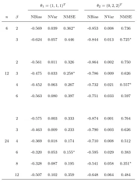
Table 1: Approximates of the NBias, NVar and NMSE for MBB estimators ˆσ2 1 = ˆσ
2 1(β)
based on exponential covariogram. The asterisk (*) denotes the minimal value of MSE.
θ1= (1,1,1)T θ2= (0,2,2)T
n β NBias NVar NMSE NBias NVar NMSE 6 2 -0.569 0.039 0.362∗
-0.853 0.008 0.736 3 -0.624 0.057 0.446 -0.844 0.013 0.725∗
2 -0.561 0.011 0.326 -0.864 0.002 0.750 12 3 -0.475 0.033 0.258∗
-0.786 0.009 0.626 4 -0.452 0.063 0.267 -0.732 0.021 0.557∗ 6 -0.563 0.080 0.397 -0.751 0.033 0.597
2 -0.575 0.003 0.333 -0.874 0.001 0.764 3 -0.463 0.009 0.233 -0.790 0.003 0.626 24 4 -0.369 0.018 0.174 -0.710 0.008 0.512
6 -0.320 0.053 0.155∗
Table 2: True values ofσ2
1and approximates of the NBias, NVar and NMSE for MBB and
SPB estimators ˆσ2
1 based on exponential covariogram.
θ1= (1,1,1)T θ2= (0,2,2)T
Method n σ2
1 βopt NBias NVar NMSE σ21 βopt NBias NVar NMSE MBB 6 5.279 2 -0.572 0.039 0.366 19.994 3 -0.846 0.014 0.729
SPB -0.254 0.295 0.359 -0.327 0.367 0.474
MBB 12 6.311 3 -0.471 0.033 0.254 32.074 4 -0.740 0.021 0.569
SPB -0.059 0.239 0.242 -0.067 0.343 0.347
MBB 24 6.890 6 -0.310 0.054 0.150 40.598 8 -0.558 0.057 0.369
SPB 0.012 0.142 0.143 0.039 0.193 0.195
Table 3: True values ofσ2
1and approximates of the NBias, NVar and NMSE for MBB and
SPB estimators ˆσ2
1 based on spherical covariogram.
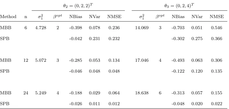
θ2= (0,2,2)T θ3= (0,2,4)T
Method n σ2
1 βopt NBias NVar NMSE σ 2
1 βopt NBias NVar NMSE MBB 6 4.728 2 -0.398 0.078 0.236 14.069 3 -0.703 0.051 0.546
SPB -0.042 0.231 0.232 -0.302 0.275 0.366
MBB 12 5.072 3 -0.285 0.053 0.134 17.046 4 -0.493 0.063 0.306
SPB -0.046 0.048 0.048 -0.122 0.120 0.135
MBB 24 5.249 4 -0.188 0.029 0.064 18.638 6 -0.313 0.057 0.155
[image:20.612.111.508.418.608.2]Table 4: True values ofσ2
1and approximates of the NBias, NVar and NMSE for MBB and
SPB estimators ˆσ2
1 based on unknown covariogram.
weak dependence strong dependence
Method n σ2
1 βopt NBias NVar NMSE σ21 βopt NBias NVar NMSE MBB 6 2.593 2 -0.125 0.124 0.140 35.637 3 -0.927 0.004 0.863
SPB -0.026 0.101 0.102 -0.620 0.353 0.737
MBB 12 3.896 3 -0.032 0.031 0.032 78.315 4 -0.880 0.006 0.781
SPB -0.011 0.013 0.013 -0.482 0.465 0.697
MBB 24 4.681 4 -0.006 0.009 0.009 126.930 8 -0.754 0.024 0.592
SPB -0.003 0.004 0.004 -0.422 0.349 0.527
Table 5: True values ofσ2
2and approximates of the NBias, NVar and NMSE for MBB and
SPB estimators ˆσ2 2.
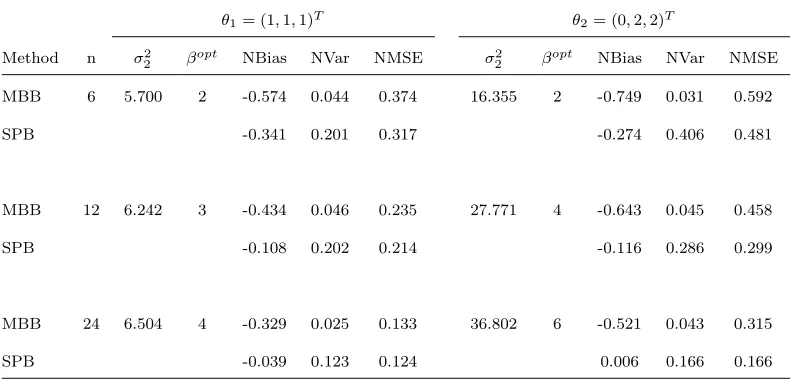
θ1= (1,1,1)T θ2= (0,2,2)T
Method n σ2
2 βopt NBias NVar NMSE σ 2
2 βopt NBias NVar NMSE MBB 6 5.700 2 -0.574 0.044 0.374 16.355 2 -0.749 0.031 0.592
SPB -0.341 0.201 0.317 -0.274 0.406 0.481
MBB 12 6.242 3 -0.434 0.046 0.235 27.771 4 -0.643 0.045 0.458
SPB -0.108 0.202 0.214 -0.116 0.286 0.299
MBB 24 6.504 4 -0.329 0.025 0.133 36.802 6 -0.521 0.043 0.315
[image:21.612.110.508.418.608.2]Table 6: True values ofσ2
3and approximates of the NBias, NVar and NMSE for MBB and
SPB estimators ˆσ2 3.
θ1= (1,1,1)T θ2= (0,2,2)T
Method n s0 σ23 βopt NBias NVar NMSE σ 2
3 βopt NBias NVar NMSE MBB 6 (3.5,3.5) 0.496 2 -0.386 0.404 0.553 1.530 2 -0.510 0.133 0.393
SPB -0.297 0.414 0.503 -0.372 0.168 0.306
MBB 12 (6.5,6.5) 0.415 3 -0.212 0.252 0.297 1.436 4 -0.215 0.114 0.160
SPB -0.128 0.265 0.282 -0.111 0.087 0.099
MBB 24 (12.5,12.5) 0.381 8 -0.036 0.132 0.133 1.385 8 -0.068 0.059 0.063
SPB -0.018 0.115 0.115 0.001 0.036 0.036
on a bootstrap sample Z∗ by T∗
3 =Z∗(s0) = ˆλTZ∗.
280
The MBB and SPB estimators ˆσ2
2 = NVar∗(µ∗) and ˆσ32 = Var∗[Z∗(s0)]
281
are approximated based onB = 1000 bootstrap replicates (9). Tables 5 and
282
6 show true values ofσ2
2 andσ32, estimates of the NBias, NVar and NMSE for
283
MBB (based on βopt) and SPB estimators ˆσ2
2 and ˆσ32 based on exponential
284
covariogram for each region D and covariogram parametersθ1 and θ2.
285
Example 4. Covariogram parameters estimator 286
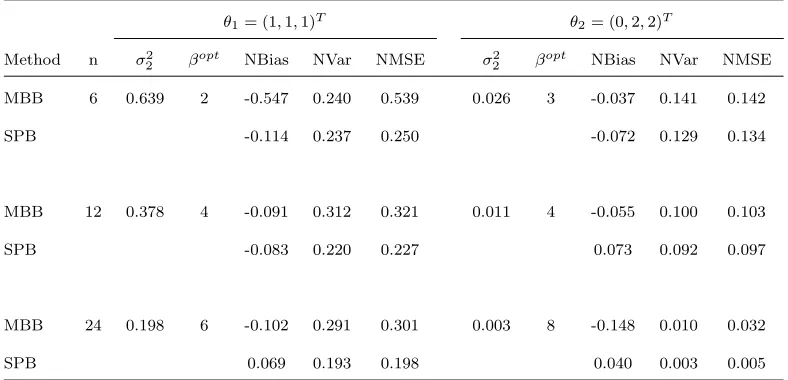
Let ˆθ = (T4, T5, T6) = (ˆc0,ˆc1,aˆ) be the MLEs of the covariogram parameters
287
θ = (c0, c1, a). Note that the estimator of ˆθ is computed numerically based
Table 7: True values ofσ2
4and approximates of the NBias, NVar and NMSE for MBB and
SPB estimators ˆσ2 4.
θ1= (1,1,1)T θ2= (0,2,2)T
Method n σ2
2 βopt NBias NVar NMSE σ 2
2 βopt NBias NVar NMSE MBB 6 0.639 2 -0.547 0.240 0.539 0.026 3 -0.037 0.141 0.142
SPB -0.114 0.237 0.250 -0.072 0.129 0.134
MBB 12 0.378 4 -0.091 0.312 0.321 0.011 4 -0.055 0.100 0.103
SPB -0.083 0.220 0.227 0.073 0.092 0.097
MBB 24 0.198 6 -0.102 0.291 0.301 0.003 8 -0.148 0.010 0.032
SPB 0.069 0.193 0.198 0.040 0.003 0.005
on the spatial sample Z as Ti = ti(Z); i = 4,5,6 and has no closed form, 289
so σ2
i = Var(Ti) is unknown. We define a version Ti∗ = ti(Z∗) of the esti-290
mator Ti based on bootstrap samples Z∗. The MBB and SPB estimators 291
ˆ
σ2
i = Var∗(Ti∗) are approximated based on B = 1000 bootstrap replicates 292
(9). Tables 7–9 show true values of σ2
i, estimates of the NBias, NVar and 293
NMSE for MBB (based onβopt) and SPB estimators ˆσ2
i based on exponential 294
covariogram for each region D and covariogram parametersθ1 and θ2.
295
Results 296
Tables 1–9 show that the MBB variance estimations ˆσ2 are underestimated.
Table 8: True values ofσ2
5and approximates of the NBias, NVar and NMSE for MBB and
SPB estimators ˆσ2 5.
θ1= (1,1,1)T θ2= (0,2,2)T
Method n σ2
2 βopt NBias NVar NMSE σ22 βopt NBias NVar NMSE MBB 6 0.863 2 -0.655 0.233 0.662 0.686 2 -0.363 0.764 0.896
SPB -0.120 0.258 0.272 -0.297 0.689 0.777
MBB 12 0.409 3 -0.118 0.288 0.302 0.246 4 -0.309 0.702 0.797
SPB -0.084 0.181 0.188 -0.273 0.507 0.581
MBB 24 0.203 4 -0.145 0.2775 0.298 0.078 6 -0.294 0.624 0.710
SPB -0.074 0.139 0.144 0.220 0.358 0.406
Table 9: True values ofσ2
6and approximates of the NBias, NVar and NMSE for MBB and
SPB estimators ˆσ2 6.
θ1= (1,1,1)T θ2= (0,2,2)T
Method n σ2
2 βopt NBias NVar NMSE σ 2
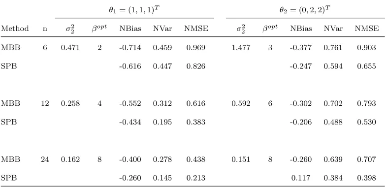
2 βopt NBias NVar NMSE MBB 6 0.471 2 -0.714 0.459 0.969 1.477 3 -0.377 0.761 0.903
SPB -0.616 0.447 0.826 -0.247 0.594 0.655
MBB 12 0.258 4 -0.552 0.312 0.616 0.592 6 -0.302 0.702 0.793
SPB -0.434 0.195 0.383 -0.206 0.488 0.530
MBB 24 0.162 8 -0.400 0.278 0.438 0.151 8 -0.260 0.639 0.707
[image:24.612.110.503.418.608.2]Tables 2–9 show that the MBB and SPB variance estimations ˆσ2 are
asymp-298
totically unbiased and consistent. Tables 2–9 also indicate that the SPB
299
estimators are preferable to the MBB versions, especially for stronger
de-300
pendence structure and larger sample sizes. In Tables 5–9, true values of
301
σ2
i = Var(Ti); i = 2,· · ·,6 have no closed form and they can be approxi-302
mated based on Monte-Carlo simulation by 10000 times replicates.
303
6. Analysis of Coal-Ash Data 304
In this section, we apply the SPB method to analyze the coal-ash data
305
(Cressie, 1993) from Greene County, Pennsylvania. These data are collected
306
with sample sizeN = 206 at locations{Z(x, y) :x = 1, . . . ,16;y= 1, . . . ,23}
307
with west coordinates greater than 64 000 ft; spatially this defines an
approx-308
imately square grid, with 2500 ft spacing (Cressie, 1993; Fig. 2.2). Our goal
309
is estimation of bias, variance and distribution of plug-in kriging predictor
310
and variogram parameters estimator by SPB method.
311
The SPB algorithm is used to estimate and remove the correlation
struc-312
ture. To estimate the correlation structure of the residuals, first, the spherical
semi-variogram
314
γ(h;θ) =
0 ||h||= 0
c0 +c1(32||ha|| −21(||ha||)3) 0<||h|| ≤a
c0 +c1 ||h|| ≥a
(11)
is fitted to the empirical semi-variogram estimation of coal-ash data with
315
ˆ
θ = (ˆc0,ˆc1,ˆa) = (0.817,0.815,15.787). Figure 1(a) shows the fitted spherical
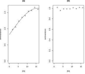
0 5 10 15
0.0
0.5
1.0
1.5
(a)
||h||
semivariance
0 5 10 15
0.0
0.2
0.4
0.6
0.8
1.0
(b)
||h||
[image:26.612.163.452.258.509.2]semivariance
Figure 1: (a) Spherical semi-variogram model ˆγ(h;θ) fitted to the empirical
semi-variogram ˆγ(h) before removal correlation structure. (b) Empirical semi-variogram
ˆ
γ(h) for standardized residuals after removal correlation structure.
semi-variogram. The covariance matrix can be estimated as ˆΣ = σ(h; ˆθ) =
317
σ(0; ˆθ)−γ(h; ˆθ). Then, the uncorrelated residuals ˆǫ = ˆL−1R are used to
318
compute the standardized uncorrelated residuals ˜ǫ(si) = (ˆǫ(si)−¯ˆǫ)/sˆǫ; i = 319
1, . . . , N. Figure 1(b) shows the fit of a linear semi-variogram to the
em-320
pirical semi-variogram estimate of the standardized residuals. The linear
321
semi-variogram model in Figure 1(b) shows that the standardized residuals
322
(˜ǫ(s1), . . . ,˜ǫ(sN)) are uncorelated. Finally, the bootstrap samples are deter-323
mined by Z∗ = ˆµ+ ˆLǫ∗, where the bootstrap vector ǫ∗ is generated by simple
324
random sampling with replacement from the standardized uncorrelated
resid-325
uals vector ˜ǫ.
326
Now suppose that the plug-in ordinary krigingT1 =Zˆˆ(s0) and variogram
327
parameter estimators ˆθ = (T2, T3, T4) = (ˆc0,cˆ1,ˆa) are the estimators of
in-328
terest, where Ti =ti(Z). For example, if s0 = (5,6) is a new location then,
329
ˆˆ
Z(s0) = ˆλTZ = 10.696 and also ˆθ = (ˆc0,ˆc1,ˆa) = (0.817,0.815,15.787). The
330
SPB version T∗
i of Ti is Ti∗ = ti(Z∗), where Z∗ is the SPB sample. We es-331
timate the precision measures Bias(Ti) and Var(Ti) and distribution GTi(t) 332
by SPB method and B bootstrap replicates T∗
i,1, . . . , Ti,B∗ ; i = 1,2,3,4 in 333
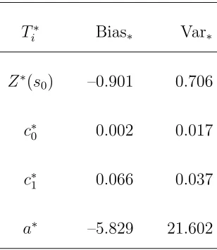
relations (8)–(10). Table 10 shows estimates of SPB bias and variance for
334
plug-in kriging and estimates of variogram parameters based on B = 1000
Table 10: Estimates of SPB bias and variance for plug-in kriging and variogram parameters
for coal-ash data.
T∗
i Bias∗ Var∗
Z∗(s
0) –0.901 0.706
c∗
0 0.002 0.017
c∗
1 0.066 0.037
a∗ –5.829 21.602
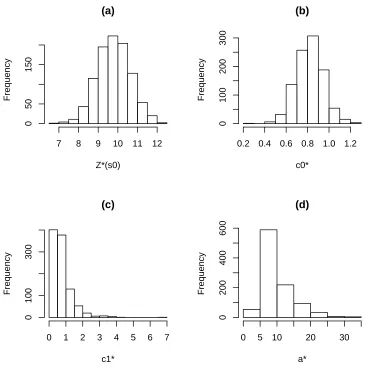
bootstrap replicates. Figure 2 shows the histogram of plug-in kriging and
336
variogram parameters estimator based on B = 1000 bootstrap replicates.
337
7. Discussion and Results 338
Spatial data analysis is based on the estimate of correlation structure, for
339
example, kriging predictor. The estimation of correlation structure is based
340
on parametric covariogram models. Unfortunately, the estimates of
covari-341
ogram parameters have no closed form and so are computed numerically. If
342
we can estimate the correlation structure as well, then we will use knowledge
343
of the covariogram model which describes the dependence structure in the
344
SPB method. For spatial data the MBB method is usually used to estimate
(a)
Z*(s0)
Frequency
7 8 9 10 11 12
0
50
150
(b)
c0*
Frequency
0.2 0.4 0.6 0.8 1.0 1.2
0
100
200
300
(c)
c1*
Frequency
0 1 2 3 4 5 6 7
0
100
300
(d)
a*
Frequency
0 5 10 20 30
0
200
400
[image:29.612.123.490.128.496.2]600
Figure 2: Histogram of (a) plug-in kriging and variogram parameters estimator:
the precision measures of the estimators. However, as already pointed out,
346
the MBB method has limitations and weaknesses. We now summarize some
347
advantages of the SPB method as compared with the MBB method:
348
The precision of the MBB estimators is related to the optimal block size
349
βopt
n in (7) which depends on unknown parameters which are difficult to 350
estimate. In our simulations it is clear that the optimal block size differs
351
for various estimators or precision measures. Note also that the optimal
352
block size determination is impossible for estimators that have no closed
353
form (e.g. covariogram parameters estimator). For some data sets we may
354
not be able to find the block size that satisfies N = Kβd
n. In other words, 355
there is not always complete blocking and then N1 =Kβnd < N is the total 356
number of data-values in the resampled complete blocks. As a result,N−N1
357
observations are ignored.
358
Establishing the consistency of MBB estimators and estimation of block
359
size requires that the random field satisfies strong-mixing conditions. In
360
the MBB method, our simulations indicate that the variance estimators ˆσ2
361
are underestimated. Moreover, our simulations show that the MBB and
362
SPB variance estimations ˆσ2 are asymptotically unbiased and consistent. In
363
this study, the SPB estimators are more accurate than the MBB estimator,
for variance estimation of estimators in spatial data analysis, especially for
365
stronger dependence structure and larger sample sizes. In the SPB method,
366
we use the estimation of spatial correlation structure, therefore the SPB
367
method will perform better than the MBB method. We are studying on
368
comparison of estimation of distribution, spatial prediction interval and
con-369
fidence interval by SPB and MBB methods.
370
Acknowledgments 371
The authors would like to thank the referees for their valuable comments
372
and suggestions. Also partial support from Ordered and Spatial Data Center
373
of Excellence of Ferdowsi University of Mashhad is acknowledged.
374
References 375
[1] Bose, A. (1988), Edgeworth correction by bootstrap in autoregression.
376
Annals of Statistics 16, 1709–1722.
377
[2] B¨uhlmann, P., K¨unsch, H.R. (1999), Comments on “Prediction of spatial
378
cumulative distribution functions using subsampling”. Journal of the 379
American Statistical Association 94, 97–99.
380
[3] Cressie, N. (1993),Statistics for Spatial Data. 2nd edn, Wiley, New York.
[4] Efron, B. (1979), Bootstrap method; another look at the jackknife.The 382
Annals of Statistics 7, 1–26.
383
[5] Efron, B., Tibshirani, R. (1993),An Introduction to the Bootstrap,
Chap-384
man and Hall, London.
385
[6] Freedman, D.A., Peters, S.C. (1984), Bootstrapping a regression
equa-386
tion: Some empirical results. Journal of the American Statistical Asso-387
ciation 79, 97–106.
388
[7] Hall, P. (1985), Resampling a coverage pattern.Stochastic Processes and 389
their Application 20, 231–246.
390
[8] Hastie, T.J., Tibshirani, R.J. (1990), Generalized Additive Models,
391
Chapman and Hall, London.
392
[9] Journel, A.G., Huijbregts, C.J. (1978), Mining Geostatistics. Academic
393
Press, London.
394
[10] Kent, J.T., Mardia, K.V. (1996), Spectral and circulant approximations
395
to the likelihood for stationary Gaussian random fields. Journal of Sta-396
tistical Planning and Inference 50, 379–394.
397
[11] Kent, J.T., Mohammadzadeh, M. (1999), Spectral approximation to the
likelihood for an intrinsic random field.Journal of Multivariate Analysis 399
70, 136–155.
400
[12] Lahiri, S.N. (2003), Resampling Methods for Dependent data,
Springer-401
Verlag, New York.
402
[13] Lahiri, S.N., Furukawa, K., Lee, Y.-D. (2007), A nonparametric plug-in
403
rule for selecting optimal block lengths for block bootstrap methods.
404
Statistical Methodology 4, 292–321.
405
[14] Liu, R.Y., Singh, K. (1992), Moving blocks jackknife and bootstrap
406
capture weak dependence, in R. Lepage and L. Billard, eds, Exploring 407
the limits of the bootstrap, Wiley, New York, pp. 225–248.
408
[15] Mardia, K.V., Marshal, R.J. (1984), Maximum likelihood estimation
409
of models for residuals covariance in spatial regression. Biometrika 71,
410
135–146.
411
[16] Mardia, K.V., Southworth, H.R., Taylor, C.C. (1999), On bias in
maxi-412
mum likelihood estimators.Journal of Statistical Planning and Inference 413
76, 31–39.
[17] Nordman, D., Lahiri, S.N. (2003), On optimal spatial subsample block
415
size for variance estimation. The Annals of Statistics 32, 1981–2027.
416
[18] Politis, D.N., Paparoditis, E., Romano, J.P. (1998), Large sample
in-417
ference for irregularly spaced dependent observations based on
sub-418
sampling. Sankhya, Series A, Indian Journal of Statistics60, 274–292.
419
[19] Politis, D.N., Paparoditis, E., Romano, J.P. (1999), ’Resampling marked
420
point processes’, in S. Ghosh, ed., ’Multivariate Analysis, Design of Ex-421
periments, and Survey Sampling: A Tribute to J. N. Srivastava’ Marcel
422
Dekker, New York, pp. 163–185.
423
[20] Politis, D.N., Romano, J.P. (1993), Nonparametric resampling for
homo-424
geneous strong mixing random fields. Journal of Multivariate Analysis 425
47, 301–328.
426
[21] Politis, D.N., Romano, J.P. (1994), Large confidence regions based on
427
subsamples under minimal assumptions. The Annals of Statistics 22,
428
2031–2050.
429
[22] Politis, D.N., Romano, J.P., Wolf, M. (1999), Subsampling,
Springer-430
Verlag, New York.
[23] Possolo, A. (1991), Subsampling a random field, in A. Possolo, ed.,
432
’Spatial Statistics and Imaging’, IMS Lecture Notes Monograph Series,
433
20, Institute of Mathematical Statistics, Hayward, CA, pp. 286–294.
434
[24] Sherman, M. (1996), Variance estimation for statistics computed from
435
spatial lattice data. Journal of the Royal Statistical Society, Series B 436
58, 509–523.
437
[25] Sherman, M., Carlstein, E. (1994), Nonparametric estimation of the
438
moments of the general statistics computed from spatial data. Journal 439
of the American Statistical Association 89, 496–500.
440
[26] Singh, K. (1981), On the asymptotic accuracy of the Efron’s bootstrap.
441
The Annals of Statistics 9, 1187-1195.
442
[27] Zimmerman, D.L., Cressie, N. (1992), Mean squared prediction error in
443
the spatial linear model with estimated covariance parameters. Annals 444
of the Institute of Statistical Mathematics 44, 27–43.