predictors of space use patterns in flocks of Amazonian
birds
Jonathan R. Potts1,2, Karl Mokross3,4, Philip C. Stouffer3,4& Mark A. Lewis1,5
1Department of Mathematical and Statistical Sciences, Centre for Mathematical Biology, University of Alberta, Edmonton, Alberta, Canada
2Department of Mathematics and Statistics, University of Sheffield, Sheffield, UK
3School of Renewable Natural Resources, Louisiana State University Agricultural Center, Baton Rouge, Louisiana 70803
4Projeto Din^amica Biologica de Fragmentos Florestais, INPA, Av. Andre Araujo 2936, Petrop olis, Manaus 69083-000, Brazil 5Department of Biological Sciences, University of Alberta, Edmonton, Alberta, Canada
Keywords
Amazon rainforest, animal movement, behavioral ecology, home range,
insectivorous birds, resource selection, space use, step selection, theoretical ecology.
Correspondence
Jonathan R. Potts, Centre for Department of Mathematics and Statistics, University of Sheffield, Sheffield, UK.
Tel: +44 (0)114 222 3729; Fax: +44 (0)114 222 3809; E-mail: [email protected]
Funding Information
This study was partly funded by NSERC Discovery and Acceleration grants (MAL, JRP). MAL also gratefully acknowledges a Canada Research Chair and a Killam Research Fellowship. JRP also acknowledges a Worldwide Universities Network Research Mobility Award. Funding for the field work was provided by US National Science Foundation grant LTREB 0545491 to PCS and by the AOU 2010 research award to KM.
Received: 9 September 2014; Accepted: 30 September 2014
Ecology and Evolution2014; 4(24): 4578– 4588
doi: 10.1002/ece3.1306
Abstract
Understanding the behavioral decisions behind animal movement and space use patterns is a key challenge for behavioral ecology. Tools to quantify these pat-terns from movement and animal–habitat interactions are vital for transforming ecology into a predictive science. This is particularly important in environments undergoing rapid anthropogenic changes, such as the Amazon rainforest, where animals face novel landscapes. Insectivorous bird flocks are key elements of avian biodiversity in the Amazonian ecosystem. Therefore, disentangling and quantifying the drivers behind their movement and space use patterns is of great importance for Amazonian conservation. We use a step selection function (SSF) approach to uncover environmental drivers behind movement choices. This is used to construct a mechanistic model, from which we derive predicted utilization distributions (home ranges) of flocks. We show that movement deci-sions are significantly influenced by canopy height and topography, but deple-tion and renewal of resources do not appear to affect movement significantly. We quantify the magnitude of these effects and demonstrate that they are help-ful for understanding various heterogeneous aspects of space use. We compare our results to recent analytic derivations of space use, demonstrating that the analytic approximation is only accurate when assuming that there is no persis-tence in the animals’ movement. Our model can be translated into other envi-ronments or hypothetical scenarios, such as those given by proposed future anthropogenic actions, to make predictions of spatial patterns in bird flocks. Furthermore, our approach is quite general, so could potentially be used to understand the drivers of movement and spatial patterns for a wide variety of animal communities.
Introduction
Understanding and quantifying the drivers behind animal movement and space use is a fundamental goal for ecology (Nathan et al. 2008). It is of particular importance in situations where landscapes are changing, making prediction vital for informed conservation (Thomas et al. 2004). The Amazon rainforest is a prime
to maintain Amazonia’s rich biodiversity (Chapin et al. 2000).
These flocks are found in practically all terra firme for-ests in the Amazon basin. They are composed of a wide variety of insectivore species that actively forage in the vegetation (Munn 1984; Powell 1989; Mokross et al. 2014). They spend practically the whole daytime searching the different strata and substrates in the vegetation, with high consumption rates. This makes them important contributors to the species richness of the Neotropical avifauna (Powell 1989).
They typically comprise at least 20 different species at any point in time and may contain as many as 60, with different species making use of various specialist niches found in the forage (Munn and Terborgh 1979). Many species are frequent flock attendants but leave occasionally (flock dropouts), either by switching between flocks, or by having smaller territories than the core species (Jullien and Thiollay 1998). However, each flock has a core composed of 5–10 species that are consistently present and share the same overlapping territory, each breeding pair defending its territory from conspecifics (Munn and Terborgh 1979). In the flocks studied here, the Cinereous Antshrike (Thamnomanes caesius) plays a nuclear role by giving alarm and rally calls that maintain flock cohesiveness (Munn 1986). Typically, movement decisions appear to be made by the Cinereous Antshrike, but occasionally, the core species fail to follow and another direction is taken.
Space use for these flocks is very stable with territory shapes changing little in two decades (Martinez and Gomez 2013). The core species gather in the same loca-tion at dawn every day, usually in a central posiloca-tion within its territory and will begin foraging from there until sunset where they roost in relatively close vicinity to each other (Powell 1985; Jullien and Thiollay 1998; Marti-nez and Gomez 2013). The purpose of this paper is to begin a process of disentangling the behavioral drivers behind these movement paths, then to use this under-standing to build a predictive model of space use patterns in insectivore bird flocks.
Linking animal movement to space use in a quantita-tive, analytic fashion is vital for predicting the effects of environmental changes on animal populations (Morales et al., 2010). The factors driving the animals’ movement ultimately determine the size and structure of the space that they use in order to meet their everyday needs. By uncovering how these movement processes give rise to spatial patterns, it would be possible to predict the types of terrain that would be used were the environment to be perturbed, by anthropogenic effects or otherwise (Nathan et al. 2008).
In this paper, we make an important step toward this end, by identifying and quantifying some of the key
environmental factors that influence Amazonian bird flock movement, then using them to construct a predic-tive model of space use. Our approach begins by using a step selection function (SSF) (Fortin et al. 2005) to test three hypotheses regarding the drivers behind the flocks’ movement decisions. Such techniques, recently reviewed by Thurfjell et al. (2014), have proved invaluable for determining the different drivers of movement in various animal populations. These include foraging decisions in elk (Forester et al. 2009), memory processes in bison (Merkle et al. 2014), mechanisms for coexistence of large carnivores (Vanak et al. 2013), and wolf–ungulate preda-tor–prey interactions (Latombe et al. 2013).
We then derive a master equation from the SSF to link these processes to the emergent space use patterns, fol-lowing the program started by Moorcroft and Barnett (2008) to integrate resource selection and mechanistic ter-ritorial models. The hypotheses we test are that (1) flocks are more likely to move into areas with taller canopies than shorter, (2) flocks tend to move away from higher ground and toward lower, (3) flocks leave some time for the resources to renew before revisiting a tree they have recently visited.
Taller canopies are expected to be preferable for birds as they tend to contain a larger mass of resources (Basset et al. 1992). Furthermore, both leaf abundance and tree height are known to be positively correlated with insect biomass in certain rainforest trees (Ellwood and Foster 2004; Campos et al. 2006). In the system studied here, some birds have been seen moving all the way up to the subcanopy and foraging there (Karl Mokross., Philip Stouffer. pers. obs.), suggesting that the flocks are making use of the entirety of each tree, so benefitting from the greater available biomass in taller trees. On the other hand, lower ground can support more buffered condi-tions from wind turbulence and sunlight from outside the forest cover (Ewers and Banks-Leite 2013) and naturally hold higher air and soil moisture levels (Baraloto and Couteron 2010) which could potentially increase arthro-pod loads per vegetation volume (Williams-Linera and Herrera 2003; Chan et al. 2008).
harder to disentangle the relative effects of each model parameter on the resulting space use.
That said, the relative effects of canopy height and topography on movement are interesting in themselves. Indeed, prior to the study, we were unclear whether the two effects were too closely related to be distinguishable. For example, it is known that tree mortality is correlated with steeper slopes in this part of the Amazon (de Casti-lho et al. 2006), so there is an expectation of more distur-bance, hence lower canopies, in steeper areas. Trees may also be shorter on slopes due to leaching of soil minerals. One outcome of the hypothesis testing will be to see whether both parameters are having an individual and separate effect on bird movement, or whether their effects are closely correlated.
Materials and Methods
The step selection function model
Our model for bird flock movement is based on a step selection function (SSF) approach (Fortin et al. 2005). Following the formalism initiated by Rhodes et al. (2005), but extended here to take into account correlations in the movement, we write the probability f(x|y, h0) of finding an animal at position x, having traveled from y in the previous step, given that it arrived atyon a bearing ofh0 as follows
fðxjy;h0Þ ¼R Uðxjy;h0Þwðx;EÞ
XUðx0jy;h0Þwðx0;EÞdx0
(1)
Here, w(x, E) is a weighting function that depends upon the animal’s positionxand some environmental co-variatesE(Forester et al. 2009),Φ(x|y,h0) is the probabil-ity of being atx in the absence of habitat selection, given that the animal was previously at yand had arrived there on a bearing of h0, Ω is the study area, and bearings are measured in an anti-clockwise direction from the right-hand half of the horizontal axis. Each step takes a fixed amount of time s. The functionΦ (x|y, h0) allows us to take into account the fact that animals may be more likely to take steps of a particular length, and the distribution of such lengths can be derived from empirical data. For com-putational purposes, we truncated the step length distribu-tion at steps of>100 m, as these never occur in our data. We include the angleh0into this formulation to allow for the possibility of correlations between successive move-ment bearings.
For the purpose of testing hypotheses (1) and (2), w (x, E) is a function of the canopy height C(x) and the topography (i.e., elevation above sea level) T(x), both
measured in meters (m). We test two candidate formula-tions forw(x,E)
waðx;a;bÞ ¼exp½aCðxÞ bTðxÞ (2)
wbðx;a;bÞ ¼CðxÞaTðxÞb (3)
Notice that eq. 3 can also be written as wbðx;a;bÞ ¼exp½alnðCðxÞÞ blnðTðxÞÞ, in keeping with the origi-nal formulation of the step selection function from Fortin et al. (2005). As we would expect the birds to be more likely to move toward lower ground than higher, we place a minus sign before the b in each equation, so thatb is expected to be positive. We treat canopy height and topography as two separate variables, noting that there is little or no correlation between the two (R2 =0.007).
To test hypothesis (3), we assume that the resource amount (i.e., insect biomass) at the start of the day (t=0) is proportional to the canopy height. This rela-tionship was observed by Campos et al. (2006), who gave linear relationships between tree height and biomass for various insect species. As the birds move through an area, they deplete the resources, which take a timeGsto renew. The resource amount present at a site at time gs after having been visited is assumed to beR(x, t,G)=gC(x)/G as long as g< G, otherwise R(x, t, G)=C(x). Here, t is the time since start-of-day, and a unit of resources is implicitly defined to be the maximum amount of usable resources sustainable by a tree per meter of tree height. At time t =0, we assume R(x, 0, G) =C(x). As with hypotheses (1) and (2), we test two candidate formula-tions forw(x,E)
wcðx;t;a;b;GÞ ¼exp½aRðx;G;tÞ bTðxÞ (4)
wdðx;t;a;b;GÞ ¼Cðx;t;GÞaTðxÞb (5)
Notice that when G=1, we have waðx;a;bÞ ¼ wcðx;t;a;b;1Þandwcðx;a;bÞ ¼wdðx;t;a;b;1Þ.
Data collection methods
maintained to an accuracy of a few meters. Where possi-ble, we used the location of a Cinereous Antshrike as the flock location. This species was usually conspicuous in the center of the flock. Other more active species typically spread out over a radius of 5–10 m, depending on the size and speed of the flock.
Although GPS error can be around 10 m, it is mainly caused by the relatively slow movement of the ionosphere (Parkinson and Spilker 1996) which only changes by a few centimeters during 30-sec intervals. Indeed, evidence from using hand-held GPS for tracking butterflies sug-gests that the median drift (i.e., absolute error) between consecutive 15-sec relocations is only 8 cm (Severns and Breed 2014). Therefore, it is reasonable to assume that the measured step lengths and turning angles accurately reflect reality.
Compared to other available methods, these data reflect well the movement of flocks on a small spatio-temporal scale. They provide a high resolution of time sequence that is not possible in radio-telemetry studies, and pres-ently, no other techniques allow the gathering of detailed spatial data for passerines of this size. Unlike remote telemetry, this method also allows the direct observation of behavior, so the observer can directly verify whether the recorded spatial locations are corresponding well with the canopy height and topographical maps.
For measuring canopy heights, we used a LIDAR (Light Detection and Ranging) canopy height model (CHM). Similarly, topography (Digital Elevation Models DEM) was acquired using small footprint airborne LIDAR. The derived (postprocessed) images from the LIDAR data are 1 m/pixel resolution, which we transformed into 10 m lattices by bilinear interpolation. LIDAR data were col-lected by airborne laser scanning using a Hexagon-LEICA ALS50 PHASE II MPiA sensor of 150 kHz, at 800 m alti-tude, with 24 degrees opening, 118 MHz pulse rate, 58 Hz scan rate, 3,7 points/m2 density. Swaths were of 340 m wide, spaced at 240 m. Postprocessing used a for-est service methodology to generate DEM and CHM at 1 m2/pixel [see Stark et al. (2012) for more details on LIDAR data collection and analysis].
Sampling was restricted to areas within LIDAR cover-age which did not span more than 1.5 km2, and of which five were scattered along the study area at an average of 6 km from each other. The choice of flocks was mainly restricted to locations where the entire home range would be inside this LIDAR coverage (i.e., away from edges of the canopy height models and digital elevation models). We analyzed six different flocks from the Dimona LIDAR dataset, which was the largest (2.8 km by 1.5 km) and best-sampled area, and also the one that presented the highest variability in vegetation types. This area falls within the Biological Dynamics of Forest Fragments
Project (BDFFP), about 70 km north of Manaus, Brazil (see http://pdbff.inpa.gov.br/ for maps).
Data were gathered during the dry seasons between June and November during 2009–2011, and each flock was tracked for between 5 and 11 days. Each flock gathers in one particular place each day, then moves around the forest for a total of about 11.5 h during the day, before each bird goes back to its roost for the night. Flock com-position was sampled every half hour to check that cohe-siveness was being maintained. Flocks were taken from a variety of different habitat types to ensure the greatest generality in our findings and minimize the effects of spa-tial autocorrelation. These included areas predominated by secondary forests, areas of primary forest away from edges, and areas near forest edges. Flocks were initially found based on their dawn gatherings. As they were first followed, it was unclear where they would go, so it is unlikely there was a bias to the flocks chosen. If the flocks moved into areas that were difficult for the observer to reach, bearings in relation to the observer were taken in order to make the necessary corrections in the data. In these cases, the observer did not lose the flock from sight.
Parametrizing the models from the data
The first step in parametrizing the models is to calculate the step length and turning angle distributions, that is, the distance between successive positions and the angle an animal turns through from one move to another, respectively [see e.g. Crist et al. (1992)]. As these depend upon the temporal resolution s (i.e., the time between successive position fixes), we use both s=1 min and s=5 min, deriving two different sets of step length and turning angle distribution for the different values of s. The value s =1 min is chosen because bird flocks tend to move from one tree to another at an average of approximately every 1 or 2 min. Although their move-ment is a continuous rather than discrete process, the model is formulated so that this timescale roughly repre-sents the small-scale decisions that the birds make regard-ing whether they stay in a tree or choose to move to another. We also examine the case s=5 min to deter-mine whether the decisions about where to move can instead be viewed as taking place on a timescale longer than a single jump between trees. In other words, the birds might only be considering the next tree they move to when deciding where to go (s =1 min), or they might be thinking a few trees ahead when they make this deci-sion (s=5 min).
determine the best model, whereas we fit the turning angles to a von Mises distribution (Marsh and Jones 1988). The Weibull, EW, and von Mises distributions have the following forms, respectively:
q1ðxja;bÞ ¼a b
x b
a1
exp x b
a
h i
; (6)
q1ðxja;b;cÞ ¼ac b
x b
a1
exp x b
a
h i
1exp x b
a
h i
n oc1
;
(7)
Vð/jkÞ ¼exp½kcosð/Þ
2pI0ðkÞ : (8)
As the rainforest canopy consists of distinct treetops whose widths are each roughly 10 m across, we split the terrain Ω into a grid S of 10m by 10m squares. This allows us to associate a value of C(s) and T(s) to each square s in S, respectively, the mean canopy height and mean topography of the square. Canopy heights ranged from 50 m to essentially none, which we set to be 1 m for the purpose of the model (a value of zero meters for the canopy height would give an identically zero probabil-ity of moving there, which is biologically implausible). Topography ranged from 40 to 115 m. Parametrizing eq. 1 from the data therefore requires maximizing the follow-ing likelihood function
LðXjEÞ ¼Y
N
n¼2
Uðxnjxn1;hn1Þwðxn;EÞ
P
s2Sðsjxn1;hn1Þwðs;EÞ (9)
where X= {x0, x1, . . ., xN}are the consecutive positions
of a flock, hn is the bearing from xn1 to xn, / is the
product of the best-fit step length and turning angle dis-tributions, and w is either wa, wb, wc, or wd, depending
on which model we are fitting.
To test hypothesis (1), we fixb=0 and find the value of a that maximizes L(X|E), which we call am. We then
use the likelihood ratio test to compare the resulting value of L(X|E) with the value of L(X|E) when both a and bset to zero. For hypothesis (2), we fix a= am and
find the value of b that maximizes L(X|E), again using the likelihood ratio test to compare this value of L(X|E) with the one wherea=amand b=0.
This technique of fixing a=am when testing
hypothe-sis (2) means that we are only testing for topographical effects on movement that are additional to the effects of canopy height. This is to address the question of whether these effects can be separated (see the last para-graph of the Introduction). We then find the values of a and b that maximize L(X|E) by varying both parame-ters simultaneously, giving best-fit values denoted by abf and bbf. We use a Markov bootstrap method with 100
bootstraps to find standard errors for a and b (Horo-witz 2003).
Hypothesis (3) is tested by fixing a= abf and b=bbf and finding the value of G that maximizes L(X|E), then using the likelihood ratio test to compare the resulting value of L(X|E) with the value of L(X|E) whenG=1. For each maximization calculation, we use the Nelder-Mead simplex algorithm (Lagarias et al. 1998), as implemented in the Python maximize() function from the SciPy library (Jones et al. 2001).
Constructing the space use distribution
We use two methods for constructing the space use dis-tribution from the parametrized SSF (eq. 1), via simula-tion analysis and through constructing the master equation and numerically deriving its steady-state solu-tion. For the former approach, we simulate one particu-lar flock’s movement on the grid S using the jump probabilities given by SSF. As the flock gathers in one particular place each day and moves around the terrain for a total of about eleven-and-a-half hours during the day, we start the simulated birds at the gathering point and run the simulation for 138 time steps, each step rep-resenting s= 5 min (giving 11 h 30 min in total), taking a note of all the positions at which the flock landed after each step. We repeat this 100 times, representing 100 days, giving 13,800 simulated positions in total. In the data, we tend to have around 10 days per flock. However, we use 100 here to average out some of the stochasticity. From these simulated positions, we calculate the 50%, 60%, 70%, 80%, and 90% Kernel density estimators (KDEs), using a fixed kernel method with smoothing parameter h=rn1/6 where r¼ð1=2Þ ffiffiffiffiffiffiffiffiffiffiffiffiffiffiffir2
xþr2y
q
and rx, ry are the standard
devia-tions of the simulated data in the x- and y-directions, respectively (Worton 1989). KDE calculations are per-formed using Python.
In addition to simulation analysis, we also construct the master equation for the probability density function u (x, h, t) of the animal being at x at time t having traveled there on a bearing of h. This allows us to compare our results with the predictions of Barnett and Moorcroft (2008), who mathematically analyzed the step selection function (eq. 1) in the simpler case where the turning angle distribution is uniform. They proved that the steady-state (time-independent) solution u*(x) is proportional to
uðx;h;tþsÞ ¼ Z p
pdh0
Z rmax
0
drR UðxjyhðrÞ;h0Þwðx;EÞ
Xdx0Uðx0jyhðrÞ;h0Þwðx0;EÞ
uðyhðrÞ;h0;tÞ
(10)
where yh(r) describes the locus of points y upon which
the animal could approach x=(x1,x2) at bearing h, that is, yh (r) =(x1+cos (h+p)r,x2+sin (h +p)r), with r
denoting the distance between yh (r) and x (Potts et al.
2014). Here,rmax is the distance along this line fromxto the boundary of Ω and so gives the upper endpoint of integration. To calculate the steady-state distribution, we solve eq. 10 iteratively until |u(x, h, t+s) u (x,h, t)|<108 for every value of x and h. The area Ω for this calculation is defined to be the 95% KDE of the flock used for the simulations. We used zero-flux bound-ary conditions, which models the fact that the birds are confined within their territory. Calculations were coded in C and it took approximately 2 h to find a single steady-state distribution.
Note that in these methods, we are separating the fit-ting of the turning angle and step length distributions from the fitting of the weighting functions. This makes the maximization procedure far faster and means the algorithms are more likely to converge to the global maxi-mum. However, if the weighting functionw gives a par-ticularly strong selection for an environmental covariate and/or the step length distributions are fat-tailed, then this separation may cause inaccuracies in the resulting model. To test that this is not the case, we calculated the
mean and standard deviation of the step length and turn-ing angle distributions from the above simulations to ver-ify that the weighting function had not significantly altered them.
Results
Step length and turning angle distributions
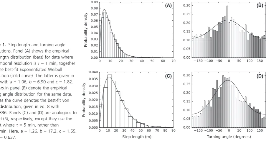
For both cases s=1 min and s =5 min, the best-fit step length distribution is an Exponentiated Weibull (EW) distribution (Fig. 1). For s=1 min, DAIC =126.9 between EW and Weibull. For s =5 min, DAIC=14.6. The step length distributions both increase from 0m ini-tially, before decaying (Fig. 1). However, this is not an indicator that birds are more likely to move a medium length distance than a very short distance, but is simply due to there being less area in the annulus of radius between r and r+dr when r is smaller. If dr is small, then the total amount of area into which a flock can move, given that it moves a distance between r and r+dr, is approximately dr92pr, which is proportional to r. To find the relative preferences of the birds to move a particular distance, it is therefore necessary to divide the probability density, P(r), by the distance moved, r. If we do this for our data on the 1 min tem-poral resolution, we find that P(r)/r is approximately 0.044 exp(r/4.75) and for the 5 min timescale P(r)/r 0.0080 exp(r/11.3), both of which decay monotonically asr increases.
(A) (B)
[image:6.595.78.530.464.703.2](C) (D)
Figure 1. Step length and turning angle distributions. Panel (A) shows the empirical step length distribution (bars) for data where the temporal resolution iss=1 min, together with the best-fit Exponentiated Weibull distribution (solid curve). The latter is given in eq. 7, witha=1.06,b=6.90 andc=1.82. The bars in panel (B) denote the empirical turning angle distribution for the same data, whereas the curve denotes the best-fit von Mises distribution, given in eq. 8 with
k=0.336. Panels (C) and (D) are analogous to (A) and (B), respectively, except they use the dataset wheres=5 min, rather than
Hypothesis testing
The tests indicate that there is a significant effect of both canopy height (hypothesis 1) and topography (hypothesis 2) on the flocks’ movement (Table 1). Furthermore, these aspects of the landscape each affect bird movement sepa-rately, rather than being highly intertwined. However, accounting for resource renewal, so that birds are less likely to revisit trees that they have recently visited, does not improve the model fit (hypothesis 3). The conclu-sions are the same both fors =1 min ands =5 min, so we cannot conclude anything about the temporal resolu-tion on which decisions are made.
To put these in a biological context, consider two trees, equally accessible over a 5-min interval and on ground of equal elevation, but one A% taller than the other. For example, if one is 30 m high and the other 20 m high then A=50. Then, the birds are (1+ A/ 100)0.277=1.50.2771.1 times more likely to move to the taller tree than the shorter, that is, about 10% more likely. The effect is more dramatic when considering the difference between a completely deforested area with essentially no canopy (which we set to 1 m for the pur-poses of the model) and primary forest with, say, 30 m canopy. Here, A= 3000, so the flocks will be around 160% more likely to move to the primary forest.
Conversely, suppose that both trees are of equal height but one tree is groundB% higher above sea level than the other. Then, the birds are (1+B/100)1.697times more likely to move to the tree on lower ground. For example, an decrease from 50 to 40 m elevation leads to a 1.251.6971.460 increase in probability of moving there, that is, they are 46% more likely to move to the 40 m elevation.
The weighting functionwb(eq. 3) provides a better fit
to the data than wa (eq. 2) for s=5 min. The AIC for
wb is lower than that forwa (DAIC=3.8). Although the
AIC for wb for s= 1 min is slightly lower than for wa
(DAIC =0.1), the change in AIC is not large enough to be considered good evidence thatwbis better than wa. In
Table 1, we detail the results for the function wb and its
generalization wd (eq. 5). Results for wa and wc (eq. 4)
are qualitatively similar.
Space use distributions
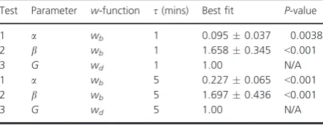
Figure 2 compares the simulated space use with the empirical data on flock positions. The KDE contour lines for the simulated data are quite tightly packed around the edge of the empirical data points, suggesting that the model is giving a reasonable prediction of space use pat-terns. However, the extent of the simulated home range is clearly larger than the empirical home range.
Although separating the fitting of the step length and turning angle distributions from the environmental inter-actions may mean that the fit is less accurate than if all parameters were fitted together, it turns out that the mean of the simulated data’s step length distribution is 20.050.95 m (95% confidence intervals), compared with 20.09 m from the data. The standard deviation of the simulated step lengths is 13.552.01 m as compared with 13.23 m from the data. Similarly, the standard devi-ation of the turning angles from simuldevi-ation output is 82.1 8.7 degrees as compared with 82.7 degrees from the data, and the mean is 0.2 6.9 degrees, as com-pared with1.7 degrees from the data. Therefore, includ-ing the weightinclud-ing function does not significantly change the step length or turning angle distributions.
Comparison with analytic results
Previous work showed that if there is no correlation in an animal’s movement, the steady-state space use distribution is proportional to w(x, E)z(x, E) as long as the turning angle distribution is uniform (Barnett and Moorcroft 2008; eq. 13), wherez(x,E)= ∫ΩΦ(x0|x, h0)w(x, E)dx0. By
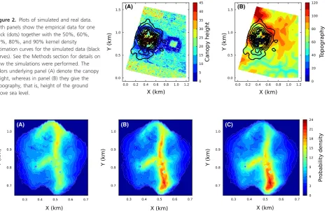
numerically deriving the steady space use distribution for our model, we show that this result breaks down when we include correlation in the movement process. Figure 3A and B compare the analytic result to the numerical one in the specific example of our Amazonian bird flock model, in the case wðx;EÞ ¼wbðx;a;bÞ (see eq. 3). However, if we assume that the turning angle distribution is uniform, then the analytic solution is very similar (Fig. 3B and C).
Discussion
[image:7.595.66.293.611.699.2]We have constructed a step selection function (SSF) to test three hypotheses about the drivers behind Amazonian Table 1. Results of hypothesis testing. The first column is number of
the test, as given in the introduction. This test finds the best-fit parameter given in the second column. The third column denotes the weighting function used for the test (see Eqs. 2–5) and the fourth gives the value of the time s between successive position measure-ments in the data. The fifth column shows the value of the parameter that fits the data best (standard error), with aP-value from the likeli-hood ratio test (see Methods) given in the sixth column and the results of a 1% significance test in the final column (note that a 5% test would give identical results).
Test Parameter w-function s(mins) Best fit P-value
1 a wb 1 0.0950.037 0.0038
2 b wb 1 1.6580.345 <0.001
3 G wd 1 1.00 N/A
1 a wb 5 0.2270.065 <0.001
2 b wb 5 1.6970.436 <0.001
bird flock movement decisions. We found that flocks have a tendency to move toward areas covered by higher canopies, but move away from areas of higher ground. The preference for higher canopies is likely to be due to the greater abundance of resources, through enhanced microclimatic conditions in the understory and more for-aging substrate (Basset et al. 1992). Lower ground is likely to be preferred because it has a moister environment that can hold a higher insect biomass (Chan et al. 2008; Bue-no et al. 2012). Although these aspects are related, we found no evidence of correlation between topography and canopy height, and each appears to have their own sepa-rate effects on flock movement.
The flocks appear to be just as likely to move back to a place that they have recently visited than one that they have not visited for a while. This suggests that when they visit a tree, they do not deplete the resources completely, but leave the tree in the knowledge that there is still food to be found there. While it may seem advantageous to stay at a tree as long as it is profitable to do so, in order
to conserve energy (Houston et al. 1993), this frequent movement from tree to tree might be a tactic to avoid predators. Alternatively, insects may temporarily be adopting cryptic behavior on the presence of birds, thus forcing the birds to move on quickly as insects become rapidly harder to find.
We tested different functional forms for the selection weighting, something that is rarely done in literature on step selection functions but could be important (Lele et al. 2013). Although we would be surprized if the functional form were to change the outcome of hypothe-sis testing, it could very much affect the resulting parameters that are used to build the mechanistic model. For example, an exponential effect of the canopy height vastly increases the relative attraction to very high cano-pies as compared with a power law effect, as this is effectively the difference between a linear and a logarith-mic scaling (see the note after eq. 3). This has the potential to vastly change the predicted space use pat-terns. Therefore, it is vital to consider functional form
[image:8.595.65.533.69.371.2](A) (B)
Figure 2. Plots of simulated and real data. Both panels show the empirical data for one flock (dots) together with the 50%, 60%, 70%, 80%, and 90% kernel density estimation curves for the simulated data (black curves). See the Methods section for details on how the simulations were performed. The colors underlying panel (A) denote the canopy height, whereas in panel (B) they give the topography, that is, height of the ground above sea level.
(A) (B) (C)
when using step selection techniques to build mechanis-tic models.
Our SSF approach enabled us to run simulations that were used to predict the utilization distribution (UD) of a flock, thereby relating the small-scale movement deci-sions to the large-scale space use patterns. While the resulting simulated UD captured certain qualitative aspects of the empirical data (Fig. 2), it overestimated the home range size. In comparison, a straightforward ran-dom walk model, based on the empirical mean step length distribution, would give a normal distribution with the 90% contour approximately 395 m from the gather-ing point. This contour would overlap the correspondgather-ing (outer) contour from Fig. 2, but would be circular, whereas the simulation contour is far from symmetric. Therefore, although certain features of space use are being predicted by our model, there must be some other aspect of the birds’ movement decisions keeping them far more spatially confined than our current model predicts.
We propose two plausible mechanisms that might explain this confinement. First, these flocks are highly ter-ritorial (Develey and Stouffer 2001), so interactions with neighboring flocks may cause each flock to use less space than they would otherwise. The mechanism of conspecific avoidance has been shown to give rise to spatial confine-ment in various species of canid (Lewis and Murray 1993; Moorcroft et al. 2006; Potts et al. 2013). These all deal with avoidance via scent marking, whereas territories in birds are defended via vocalizations and direct interac-tions (Munn and Terborgh 1979). However, the generic modeling framework from Potts et al. (2013) could be used to construct coupled SSFs, whose weighting func-tions w depend both upon the position of the individual and on interactions with neighbors. These interactions may either be direct or mediated by vocal, visual, or olfactory cues.
Second, memory effects, with birds having a preference to move back toward places they have frequently visited, can cause spatial confinement. Theoretical studies by Bris-coe et al. (2002) have described such a mechanism in wolf (Canis lupus) populations, and the general results of Tan et al. (2001) show that memory can severely con-strain the amount of area used in a given time period. Although it is tricky to determine empirically what con-stitutes a bird’s cognitive map of the environment, it is generally considered that memory is an important factor in the spatial confinement and site-fidelity of many ani-mals (Smouse et al. 2010).
By turning our SSF into a master equation for the spa-tiotemporal probability distribution of the flock’s posi-tion, we compared our results to a recent approximate analytic prediction by Barnett and Moorcroft (2008) that applies when the turning angle distribution is uniform.
However, their results fail whenever there is correlation in the animal’s movement at any timescale, a fact noted by Barnett and Moorcroft (2008) but not emphasized in their ecologically motivated paper Moorcroft and Barnett (2008). The more the correlation, the worse the predic-tion is likely to be, so it is necessary to take care when applying these results to empirical data. Although the cor-relation in the birds’ movement greatly affected the move-ment patterns, when we removed any intrinsic correlation from our movement model, the predictions of Barnett and Moorcroft (2008) were visually very good (Fig. 3).
Although our results are not testing conservation deci-sionsper se, the application of these models could provide basis for informed management decisions for a subset of the avian community that is known to be very sensitive to forest disturbances. By providing information on how a combination of two important habitat features influ-ences habitat use and how these flocks anchor their home ranges, this would allow for more realistic estimations of areas that are more important to these species. Also, the drivers related to resource abundance and renewal pro-vide important insights into the nature of the relationship of insectivorous birds and their resource, a topic that has challenged researchers for years (Sherry 1984; Sßekercioḡlu et al. 2002). These results also have the potential to be extended to closely related species in other regions of Amazonia. For example, in southwestern Amazonia, flocks are lead by T. schistogynus rather than T. caesius (Munn and Terborgh 1979) which may behave differently. It is an interesting future challenge to analyze these differ-ences rigorously. The dynamic and collective nature of bird flock decisions is also likely to have an impact on behavioral decisions. As we refine our model to make it more accurate at predicting space use, it will likely be necessary to take these effects into account.
Acknowledgments
Technical Series of the INPA Zoological Collections Pro-gram. This manuscript was approved for publication by the Director of the Louisiana Agricultural Experiment Station as manuscript 2014-241-17747. LIDAR images for canopy height models and digital elevation models were provided by Scott Saleska (University of Arizona) and Michael Lefsky (Colorado State University). We are grate-ful to Greg Breed, the Lewis Lab, and various other colleagues and anonymous referees for helpful discussions and comments.
Data Accessibility
Data can be found in Dryad doi:10.5061/dryad.47jh1.
Conflict of Interest
None declared.
References
Baraloto, C., and P. Couteron. 2010. Fine-scale microhabitat heterogeneity in a French Guianan forest. Biotropica 42:420–428.
Barnett, A. H., and P. R. Moorcroft. 2008. Analytic steady-state space use patterns and rapid computations in mechanistic home range analysis. J. Math. Biol. 57:139–159. Basset, Y., H. P. Aberlenc, and G. Delvare. 1992. Abundance
and stratification of foliage arthropods in a lowland rainforest in Cameroon. Ecol. Entomol. 17:310–318. Briscoe, B. K., M. A. Lewis, and S. E. Parrish. 2002. Home
range formation in wolves due to scent marking. Bull. Math. Biol. 64:261–284.
Bueno, A. S., R. S. Bruno, T. P. Pimentel, T. M. Sanaiotti, and W. E. Magnusson. 2012. The width of riparian habitats for understory birds in an Amazonian forest. Ecol. Appl. 22:722–734.
Campos, R. I., H. L. Vasconcelos, S. P. Ribeiro, F. S. Neves, and J. P. Soares. 2006. Relationship between tree size and insect assemblages associated withAnadenanthera macrocarpa. Ecography 29:442–450.
de Castilho, C. V., W. E. Magnusson, R. Nazare, O. de Araujo, R. C. C. Luiz~ao, F. J. Luiz~ao, et al. 2006. Variation in aboveground tree live biomass in a central Amazonian Forest: effects of soil and topography. For. Ecol. Manage. 234:85–96.
Chan, E. K. W., Y. T. Yu, Y. Zhang, and D. Dudgeon. 2008. Distribution patterns of birds and insect prey in a tropical riparian forest. Biotropica 40:623–629.
Chapin, F. S. III, E. S. Zavaleta, V. T. Eviner, R. L. Naylor, P. M. Vitousek, H. L. Reynolds, et al. 2000. Consequences of changing biodiversity. Nature 405:234–242.
Crist, T. O., D. S. Guertin, J. A. Wiens, and B. T. Milne. 1992. Animal movement in heterogeneous landscapes: an
experiment withEleodesbeetles in shortgrass prairie. Funct. Ecol. 6:536–544.
Develey, P., and P. C. Stouffer. 2001. Effects of roads on movements by understory birds in mixed-species flocks in central Amazonian Brazil. Conserv. Biol. 15:1416–1422. Ellwood, M. D. F., and W. A. Foster. 2004. Doubling the
estimate of invertebrate biomass in a rainforest canopy. Nature 429:549–551.
Ewers, R. M., and C. Banks-Leite. 2013. Fragmentation impairs the microclimate buffering effect of tropical forests. PLoS ONE 8:e58093.
Fearnside, P. M. 2005. Deforestation in Brazilian Amazonia: history, rates, and consequences. Conserv. Biol. 19:680–688. Forester, J. D., H. K. Im, and P. J. Rathouz. 2009. Accounting
for animal movement in estimation of resource selection functions: sampling and data analysis. Ecology 90:3554–3565. Fortin, D., H. L. Beyer, M. S. Boyce, D. W. Smith, T.
Duchesne, and J. S. Mao. 2005. Wolves influence elk movements: behavior shapes a trophic cascade in Yellowstone National Park. Ecology 86:1320–1330.
Horowitz, J. L. 2003. Bootstrap methods for markov processes. Econometrica 71:1049–1082.
Houston, A. I., J. M. McNamara, and J. M. C. Hutchinson. 1993. General results concerning the trade-off between gaining energy and avoiding predation. Philos. Trans. R. Soc. Lond. B 341:375–397.
Jones, E., T. Oliphant, P. Peterson, et al. 2001.SciPy: Open source scientific tools for Python. Available at http://www. scipy.org/scipylib/citing.html. (accessed 1st September 2014). Jullien, M., and J. M. Thiollay. 1998. Multi-species
territoriality and dynamic of Neotropical forest understory bird flocks. J. Anim. Ecol. 67:227–252.
Lagarias, J. C., J. A. Reeds, M. H. Wright, and P. E. Wright. 1998. Convergence properties of the Nelder-Mead simplex method in low dimensions. SIAM J. Optim. 9:112–147. Latombe, G., D. Fortin, and L. Parrott. 2013. Spatio-temporal
dynamics in the response of woodland caribou and moose to the passage of gray wolf. J. Anim. Ecol. 83:185–198, doi: 10.1111/1365-2656.12108.
Laurance, W. F., J. L. C. Camargo, R. C. C. Luiz~o, S. G. Laurance, S. L. Pimm, E. M. Bruna, et al. 2011. The fate of Amazonian forest fragments: a 32-year investigation. Biol. Conserv. 144:56–67.
Lele, S. R., E. H. Merrill, J. Keim, and M. S. Boyce. 2013. Selection, use, choice and occupancy: clarifying concepts in resource selection studies. J. Anim. Ecol. 82:1183–1191. Lewis, M. A., and J. D. Murray. 1993. Modelling territoriality
and wolf-deer interactions. Nature 366:738–740.
M€antyl€a, E., T. Klemola, and T. Laaksonen. 2011. Birds help plants: a meta-analysis of top-down trophic cascades caused by avian predators. Oecologia 165:143–151.
Marsh, L. M., and R. E. Jones. 1988. The form and
Martinez, A. E., and J. P. Gomez. 2013. Are mixed-species bird flocks stable through two decades? Am. Nat. 181:E53–E59. Merkle, J. A., D. Fortin, and J. M. Morales. 2014. A
memory-based foraging tactic reveals an adaptive
mechanism for restricted space use. Ecol. Lett. 17:924–931. Mokross, K., T. B. Ryder, M. Corr^ea C^ortes, J. D. Wolfe, and
P. C. Stouffer. 2014. Decay of interspecific avian flock networks along a disturbance gradient in Amazonia. Proc. R. Soc. B 281:20132599.
Moorcroft, P. R., and A. Barnett. 2008. Mechanistic home range models and resource selection analysis: a reconciliation and unification. Ecology 89:1112–1119. Moorcroft, P. R., M. A. Lewis, and R. L. Crabtree. 2006.
Mechanistic home range models capture spatial patterns and dynamics of coyote territories in Yellowstone. Proc. R. Soc. B 273:1651–1659.
Morales, J. M., P. R. Moorcroft, J. Matthiopoulos, J. L. Frair, J. G. Kie, R. A. Powell, et al. 2010. Building the bridge between animal movement and population dynamics. Philos. Trans. R. Soc. B 365:2289–2301.
Munn, C. A. 1984. Birds of a different feather also flock together. Nat. Hist. 93:34.
Munn, C. A. 1986. Birds that cry wolf. Nature 319:143–145. Munn, C. A., and J. W. Terborgh. 1979. Multi-species territoriality
in Neotropical foraging flocks. Condor 81:338–347. Nassar, M. M., and F. H. Eissa. 2003. On the exponentiated
Weibull distribution. Commun. Stat. Theory Methods 32:1317–1336.
Nathan, R., W. M. Getz, E. Revilla, M. Holyoak, R. Kadmon, D. Saltz, et al. 2008. A movement ecology paradigm for unifying organismal movement research. Proc. Natl Acad. Sci. USA 105:19052–19059.
Nepstad, D., D. McGrath, C. Stickler, A. Alencar, A. Azevedo, B. Swette, et al. 2014. Slowing Amazon deforestation through public policy and interventions in beef and soy supply chains. Science 344:1118–1123.
Parkinson, B. W., and Spilker J. J. 1996. Global positioning system: theory and applications. Vol. 1. AIAA, Washington, DC.
Potts, J. R., S. Harris, and L. Giuggioli. 2013. Quantifying behavioral changes in territorial animals caused by sudden population declines. Am. Nat. 182:E73–E82.
Potts, J. R., G. Bastille-Rousseau, D. L. Murray, J. A. Schaefer, and M. A. Lewis. 2014. Predicting local and non-local effects of resources on animal space use using a mechanistic step-selection model. Methods Ecol. Evol. 5:253–262.
Powell, G. V. N. 1985. Sociobiology and adaptive significance of interspecific foraging flocks in the Neotropics. Ornithol. Monogr. 36:713–732.
Powell, G. V. N. 1989. On the possible contribution of mixed species flocks to species richness in Neotropical avifaunas. Behav. Ecol. Sociobiol. 24:387–393.
Rhodes, J. R., C. A. McAlpine, D. Lunney, and H. P. Possingham. 2005. A spatially explicit habitat selection model incorporating home range behavior. Ecology 86:1199–1205.
Sßekercioḡlu, Cß. H., P. R. Ehrlich, G. C. Daily, D. Aygen, D. Goehring, and R. F. Sandı. 2002. Disappearance of insectivorous birds from tropical forest fragments. Proc. Natl Acad. Sci. USA 99:263–267.
Severns, P. M., and G. A. Breed. 2014. Behavioral
consequences of exotic host plant adoption and the differing roles of male harassment on female movement in two checkerspot butterflies. Behav. Ecol. Sociobiol. 68:805–814, doi: 10.1007/s00265-014-1693-z.
Sherry, T. W. 1984. Comparative dietary ecology of sympatric, insectivorous Neotropical flycatchers (Tyrannidae). Ecol. Monogr. 54:313–338.
Smouse, P. E., S. Focardi, P. R. Moorcroft, J. G. Kie, J. D. Forester, and J. M. Morales. 2010. Stochastic modeling of animal movement. Philos. Trans. R. Soc. B 365:1471–2970. Stark, S. C., V. Leitold, J. L. Wu, M. O. Hunter, C. V. de
Castilho, F. R. C. Costa, et al. 2012. Amazon forest carbon dynamics predicted by profiles of canopy leaf area and light environment. Ecol. Lett. 15:1406–1414.
Tan, Z.-J., X.-W. Zou, W. Zhang, and Z.-Z. Jin. 2001. ‘True’ self-attracting walk. Phys. Lett. A 289:251–254.
Thomas, C. D., A. Cameron, R. E. Green, M. Bakkenes, L. J. Beaumont, Y. C. Collingham, et al. 2004. Extinction risk from climate change. Nature 427:145–148.
Thurfjell, H., S. Ciuti, and M. S. Boyce. 2014. Applications of step-selection functions in ecology and conservation. Mov. Ecol. 2:4: doi:10.1186/2051-3933-2-4. http://www. movementecologyjournal.com/about.
Vanak, A. T., D. Fortin, M. Thakera, M. Ogdene, C. Owena, S. Greatwood, et al. 2013. Moving to stay in place–behavioral mechanisms for coexistence of African large carnivores. Ecology 94:2619–2631. doi:10.1890/13-0217.1.
Williams-Linera, G., and F. Herrera. 2003. Folivory,
herbivores, and environment in the understory of a tropical montane cloud forest. Biotropica 35:67–73.