Spatio-temporal Evolution as Bigraph Dynamics

This is a repository copy of

Spatio-temporal Evolution as Bigraph Dynamics

.

White Rose Research Online URL for this paper:

http://eprints.whiterose.ac.uk/43134/

Proceedings Paper:

Stell, JG, Del Mondo, G, Thibaud, R et al. (1 more author) (2011) Spatio-temporal

Evolution as Bigraph Dynamics. In: Egenhofer, M, Giudice, N, Moratz, R and Worboys, M,

(eds.) Spatial Information Theory, 10th International Conference, COSIT

2011.Proceedings. Conference on Spatial Information Theory, COSIT, 12-16 Sep 2011,

Belfast, Maine, USA. Lecture Notes in Computer Science, 6899 (6899). Springer , 148 -

167 (20). ISBN 978-3-642-23195-7

https://doi.org/10.1007/978-3-642-23196-4

[email protected]

Reuse

Unless indicated otherwise, fulltext items are protected by copyright with all rights reserved. The copyright exception in section 29 of the Copyright, Designs and Patents Act 1988 allows the making of a single copy solely for the purpose of non-commercial research or private study within the limits of fair dealing. The publisher or other rights-holder may allow further reproduction and re-use of this version - refer to the White Rose Research Online record for this item. Where records identify the publisher as the copyright holder, users can verify any specific terms of use on the publisher’s website.

Takedown

If you consider content in White Rose Research Online to be in breach of UK law, please notify us by

Spatio-temporal Evolution as Bigraph Dynamics

J. Stell1

, G. Del Mondo2

, R. Thibaud2

, and C. Claramunt2

1

School of Computing, University of Leeds, U.K. [email protected]

2

Naval Academy Research Institute, Brest, France

geraldine.del [email protected],[email protected] [email protected]

Abstract. We present a novel approach to modelling the evolution of spatial entities over time by using bigraphs. We use the links in a bi-graph to represent the sharing of a common ancestor and the places in a bigraph to represent spatial nesting as usual. We provide bigraphical reaction rules that are able to model situations such as two crowds of people merging together while still keeping track of the resulting crowd’s historical links.

Keywords: spatio-temporal change, bigraphs, filiation

1

Introduction

The combined modelling of space and time is a well-established aspect of the theory of spatial information [8, 12, 18, 9, 3, 2]. It also provides particular chal-lenges when dealing with granularity and vagueness [14, 4]. Objects can move, cities and countries can retain their identities while changing their boundaries, new entities can be formed from old ones as in the redistribution of parcels of parcels of land or the more rapid change seen as crowds of demonstrators are divided by police and then re-form and take on new activity. Such examples are recorded in systems having purposes as diverse as tracking the delivery of consumer goods in a postal system, the legal record of land ownership, or the surveillance of crowds of people in public demonstrations.

Despite all these, and many more examples that could be mentioned, the formal description of spatio-temporal change in a way that suits the needs of information systems is still at an early stage. In the purely spatial case, certain basic systems of spatial relationships have been found useful; the 9-intersection model [5] has acquired the status of a standard and systems for qualitative spa-tial reasoning [1], including the Region-Connection Calculus, have been very widely studied and applied. The spatial relations modelled in such systems in-clude widely accepted notions such as ‘overlapping’, ‘inside but not touching the boundary’, and ‘disjoint’.

In contrast models of spatio-temporal change, while numerous and containing much valuable work, have not reached any consensus about the atomic concepts they need to provide. We can imagine spatio-temporal scenarios between regions,

Conference on Spatial Information Theory (COSIT)

Belfast, Maine, 12-16 September 2011

such as one moving to encircle another, or two regions moving further apart to allow a third to pass between them. The most basic scenarios of single regions splitting and merging have been rigorously analysed in [9, 15], but it is not clear whether more complex behaviours can be treated in a similar way. In order to study such behaviour it is necessary to have a formal framework that is capable of modelling spatio-temporal change without pre-judging the kinds of higher level events and process that will be significant. This means that we should base our study on primitive concepts that appear to be essential and which can be combined to exhibit a variety of different behaviours. In this paper we propose that structures known as bigraphs provide what is needed. In addition to drawing the attention of the spatial information theory community to this area, we also introduce a novel way of using bigraphs to model relationships between entities in terms of shared ancestry.

Bigraphs were introduced by Milner [11] and are so called as they provide a single set of nodes having two distinct kinds of edges between them. The nodes with one kind of edge form a set of trees which allow the nodes to represent spatial nesting. This can model situations such as a person being in a room which is inside a building. The nodes taken together with the other kind of edge constitute a hypergraph where one edge may be incident with a set of nodes (not just one or two). The original motivation for bigraphs uses this hypergraph (called the link graph) as a way of modelling communication between the things represented by the nodes. For example, two nodes representing people might be joined by a link representing their participation in a phone call. In another scenario one of the hyperedges could represent a local area network, and the nodes computers connected by means of it.

The applicability of bigraphs to spatial information theory has already been noted in [16] and [7]. In [16] Walton and Worboys make extensive use of bigraphs to model image schemas. Their work proposes bigraph reaction rules to model dynamic schemas and uses bigraph composition to model change in level of detail.

The spatial relationships modelled in bigraphs are clearly restricted, as even simple overlapping of spatial entities is excluded. However, the interaction of spatial structure and communication even in this simplified case presents chal-lenges to a fully rigorous analysis, and it is appropriate to ensure the simpler setting is fully understood before proceeding to more elaborate models. There has been some work [13] on bigraphs in which a node may be shared between two distinct containing nodes, but we do not make use of this in the present paper.

process of rewriting is essentially familiar from simplifications such as replacing an instance of x+ 0 by x in an algebraic expression such as (2 + 0)y to end up with 2y. The fact that a bigraph can be written as an algebraic expression means that sequences of spatial changes have algebraic counterparts allowing these changes to be analysed in a rigorous way.

The main novelty to which we draw attention in the present work is the way in we are able to use the links in a bigraph (the edges in the hypergraph) to model shared ancestry. The idea behind this is explained in terms of relations and hypergraphs in Section 2. Bigraphs are introduced in Section 3 where, as these structures are not widely known in spatial information theory, we provide an expository account of the basic ideas and refer the reader to [11] for more details. In Section 4 we present a scenario of one kind of situation where spatio-temporal modelling is important. Our case study involves crowds of people moving in a city. The ability of bigraphs to model the essential dynamic features of this case study is demonstrated in Section 5 where we give reaction rules for changes in the location and compostion of the crowds. Finally, Section 6 provides conclusions and outlines directions for further work.

2

Relations and Summaries

2.1 Filiation

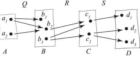
Many formal models proposed for spatio-temporal evolution involve the mathe-matical concept of a relation between two sets. If the sets areX and Y then a relation fromX toY can be visualized as a set of arrows leading from elements of X to elements of Y. These arrows are subject only to the restriction that givenx∈X andy∈Y there is at most one arrow fromxtoy. The suitability of this for modelling the most basic features of change is evident if we takeX

andY to be sets of entities at two times, the second coming after the first. Considering more times than just two we can use a sequence of sets. In Figure 1 there are four sets of entities and three relations between them. Each set represents a snapshot of the entities at a paticular time, and the relations model links between these entities and the ones present at the previous or next time in the sequence. The nature of the links will depend on the particular scenario being modelled.

To give some examples of the possible meaning of such a link we can consider Figure 1 where in relationQwe see thata1 is linked, or related, to bothb1 and

a

a

b

b

b

c

c

_d

3

d

d

Q

R

S

A

B

C

_D

Fig. 1.Three relations between four times

existence of an entity, while the link froma1 to b2 can denote the earlier entity giving rise to a separate entity (the childb2) at the later stage. We use the term

filiation for a link of any kind connecting entities in this way, and this topic has been studied further in [3].

The way in which identity continues in objects that change is a long-standing issue in philosophy [6, 17]. However, the existence of a filiation link does not nec-essarily indicate a continuation of identity. A filiation link from a parent to a child could be regarded as the continuing identity of the family, or with equal validity as the creation of a separate personal identity. The choice between these two would depend on the application domain but would be some additional structure beyond the existence of a filiation link. We do annotate the filiations to show different kinds of behaviour with respect to identity in the case study in Section 4, but in the present work this annotation is not modelled by the opera-tions on bigraphs that we describe. The continuation of identity is important in information systems [8, 10]. In [8] Hornsby and Egenhofer study operations for the construction of composite objects based on features of identity which include the creation, continuation and elimination of identity. The incorporation of this type of approach in our use of bigraphs would be an interesting direction for further work.

2.2 Summarizing Evolution

The representation of every known timepoint in the sequence and the filiation links between every successive pair of times is the highest level of detail in the model. For many purposes this level of detail can be unnecessarily complex and a less detailed, or more coarse grained, view is more approriate. In the example involving just four times with sets of entities A, B, C and D illustrated in Figure 1 we might need to summarize the change from the time ofAto that of

C. The usual way to summarize this change would be to compose the relations

QandRas in Figure 2.

In the summary by relation composition we see thatc1has botha1anda2as ancestors. The summary however has lost two pieces of information: thatc1and

a

a

c

c

Q;R

d

d

d

a

a

(Q;R) ;S

Fig. 2.Composite relations

two times evident in the summary. It is in the nature of a useful summarization technique for information to be lost, but there are practical cases where the fact that two entities shared a common ancestor would be something that it would be useful for a summary to maintain.

It is possible to define a way of summarizing a composable pair of relations that is different to their composition. The idea is that given relationsQ:A→B

andR:B→Cwe can enlargeAto include any entities inBwhich are not linked to anything inA. In the next definitionQ(A) means{b∈B | ∃a∈A(a Q b)}.

Definition 1 (Cumulative Product) Let Q : A → B and R : B → C be relations, whereAandB−Q(A)are disjoint. The cumulative product ofQand

R is the relation Q ⋆ R:A∪(B−Q(A))→C where

x Q ⋆ R ciff

(

x∈B−Q(A)and x R c, or

x∈A andx Q;R c.

Examples of this construction are shown in Figure 3. The assumption that A

andB−Q(A) are disjoint in the definition may appear restrictive. However the elements of the sets are not the individuals being modelled in the world, rather they are tokens which can be mapped to the world. This permits distinct tokens to take the same identity, and the issue here can be understood more fully by using an analysis analogous to the idea of support for bigraphs used in [11].

c

c

a

a

b

Q ⋆ R

d

d

d

a

a

b

(Q ⋆ R)⋆ S

Conceptually the cumulative product is quite distinct from composition. The composition of relations describes a process of entities changing from past to present. The cumulative product models the state in the present, looking back. This suggests the idea of a map which shows the present state of the world but also contains evidence of past history indicating how the present state arose through accumulating changes. For this reason we sometimes refer to accumula-tion instead of the cumulative product.

Note that if relationsQ,R,Sare composable so thatQ;R;S is defined then we may form the accumulation (Q ⋆ R)⋆ Sbut not, in general, the accumulation

Q ⋆(R ⋆ S). This is because the enlarged domain of R ⋆ S by the addition of elements not present in R means that the co-domain of Q may not match the domain of R ⋆ S. This behaviour is as one would expect given the way that accumulation is inherently directional, building on the past.

We can visualize a sequence of relations as follows with relationsbetween times.

X0

R1

- X₁

R2

- X₂ . . . X

n−1

Rn

- X

n

t0 t1 t2 . . . tn−1 tn

For accumulation, the picture naturally places the relationsabove the times. The relationAi describes the entities at timeti and (some of) their past history.

A1=R1

A2=A1⋆ R2

. . .An−1=An−2⋆ Rn−1

. . . An =An−1⋆ Rn

t0 t1 t2 . . . tn₋1 tn

2.3 Hypergraphs

A hypergraph can represent a view in which the entities in the present are nodes bearing additional structure (edges) which represent the past state and the way the past has become the present. We explain hypergraphs below, and then show how accumulation is seen as an operation describing the change from one time to the next.

Definition 2 AHypergraphH consists of setsVH of vertices andEH of edges

(whereVH∩EH =∅), and an incidence relationiH :EH→P(VH).

A hypergraph differs from an undirected graph in that an edge may be incident with an arbitrary set of nodes and not just one or two. Note that we do allow edges incident with the empty set of nodes,∅. A hypergraph with edges_E and

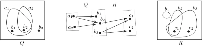
verticesV is the same as a relation fromE toV; an edge is related to the set of vertices with which it is incident. This is illustrated in Figure 4 for the relations

QandR from Figure 1. In the figure the hyperedges appear as loops enclosing their incident nodes.

a1 a2

Q R

b1 b2 b3

b1 b2 b3 a2 c1 c2

a1

b1

b2

b3

c1

c2

Q R

Fig. 4.RelationsQandRfrom Figure 1 as hypergraphs

The accumulation of two relations can be described in terms of hypergraphs.

Definition 3 Let G and H be hypergraphs where VG = EH. We define the

hypergraphG ⋆ H to have vertices VH, and edges EG∪ {v ∈VG |i−

1

G (v) =∅}.

The incidence relationj is given by

j(x) =

S

{iH(v)⊆VH |v∈iG(x)} if x∈EG

iH(x) if x∈ {v∈VG|i−

1

G (v) =∅}

3

Bigraphs: Static Aspects

In the previous section we considered entities subject to change, but without modelling any spatial relationships between these entities. If we introduce spatial structure in addition to the links representing shared ancestry between nodes then we have essentially the bigraphs introduced by Milner [11].

3.1 Bare Bigraphs

If we assume that all the entities involved (a1, a2, . . .) are spatially disjoint we arrive at Figure 5. This figure shows the usual means of depicting bigraphs with the spatial entities shown as discs in the plane and the links connecting them drawn as lines attached to the discs. This differs from the more usual way of drawing an edge in a hypergraph as a boundary containing those nodes with which it is incident. We used this edge-as-container vizualization in earlier figures with hypergraphs, but this only works when the nodes do not have a spatial extent.

Bare bigraph forQ bare bigraph forQ ⋆ R _{Bare bigraph with nesting} (assuming{b1, b2, b3, c1, c2}spatially disjoint)

Fig. 5.Examples of bare bigraphs

The examples in Figure 5 of the bigraphs for the relationsQandQ ⋆ Rare particularly simple in that the nodes are spatially disjoint. In general nodes may be nested with each other, as indicated in the example at the right of Figure 5. The place structure (that is the nesting of nodes) is independent of the link structure (that is the edges of the hypergraph part of the bigraph). This means that although it is significant when nodes are drawn inside other nodes, there is no significance attached to where the links cross the boundaries of nodes

The bare bigraph forQshown in Figure 5 has one edge (a2) that is incident with just one node. This has been drawn in the diagram as a link which has been terminated, not linking the node to anything. This follows Milner’s diagrams [11] but in other contexts such edges are often drawn as loops with both ends attached to the incident node.

3.2 Substitution

machinery to allow substitution. This means that a bigraph can be inserted into a larger context and it can also act as a context into which more detail is inserted. It may be helpful to give an analogy with simple algebra in which letters stand for numbers. A complicated expression such as (3x+ 2y)2

+ 2(3x+ 2y) + 1 can be built out of the simpler expressionz2

+ 2z+ 1 by replacingzby (3x+ 2y). Informally, the z in z2

+ 2z+ 1 acts as a ‘hole’ which can be ‘filled in’ by the expression (3x+ 2y).

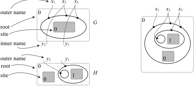
General bigraphs may contain ‘holes’ of two types called sites and inner names into which ‘fillers’ called respectively roots and outer names may be placed. These additional features are illustrated in Figure 6. The ability to com-pose bigraphs makes them morphisms in a category where the objects (known asinterfaces) are pairshm, Xiwheremis essentially the number of place holes andX is a finite set of names. The numbermis treated as a finite ordinal, that is a natural number viewed as a set of smaller ordinalsm={0,1, . . . , m−1}.

0 0

0

0

x1 x2 x3

1 y1

y1

y2

y2

outer name

outer name inner name root

site root

0

0

x1 x2 x3

1 site

G

H

Fig. 6.BigraphsG:h1,{y1, y2}i → h1,{x1, x2, x3}iandH:h2,∅i → h1,{y1, y2}iand

the compositeG◦H

Although the operations ◦ on bigraphs and ; on relations are both called ‘composition’ they are unrelated. Relations between spatially nested entities can be modelled by bigraphs and the composition of relations can thus be modelled by an operation on bigraphs. However this operation would only be defined under conditions that would be very different from the conditions under which ◦ is defined and the two operations are quite separate.

3.3 Ports

link (hyperedge) may be made for nodes of type k. These ports are shown as black discs in the diagrams. For example, in the examples we provide later we use different types of node for buildings, suburbs and crowds. In this setting the arity of a particular type of crowd is the number of instances of ‘original crowds’ whose members are present in it. It should be noted that the formal definition of bigraphs [11, p15] allows a link to be connected to the same node by a number of different ports. This means that the link structure is actually more general than a hypergraph as defined above since each edge may be incident with a multiset (or bag) of nodes and not just a set.

3.4 Tensor product and derived operations

Besides the operation of composition,◦, bigraphs also support an operation⊗ known as the tensor product. This is easy to visualize and corresponds to placing bigraphs with disjoint names alongside each other aligned horizontally.

Further operations that we use in formulating the rules later in the paper can be expressed in terms of composition and tensor product. These are the parallel product, (k), nesting (.), and the merge product (|). A full account of these operations would occupy more space than we have available, and [11] should be consulted for details. Briefly, however, GkH is similar to the tensor product except that common outer names are shared. The nestingG . HplacesH inside

G and allows the outer names of H to be visible. The merge product G|H

merges roots in addition to sharing links as in the parallel product.

3.5 Modelling Parents and Children

We introduced hypergraphs by showing how edges might represent the sharing of common ancestors between entities. When in addition entities have spatial structure limited to nesting a bigraph can represent both the filiation links and the nesting relationships. The original motivation for bigraphs uses the links to model communication of various types.

An individual person can be represented by a node with three ports where we can attach links to (1) their mother, (2) their father, (3) their children. From this example it is clear that the link structure is independent of the spatial structure: who a person is related to has no bearing on their location. It should also be noted that although the links have no specified direction, we can make use of the signature to use particular ports in particular ways. By this means we can tell for example that a link from port 3 of nodeato port 1 of nodebmeans that

ais a child ofb.

e

e

B

e3

A

e

e

Q1

Q2

Boundary between suburbs

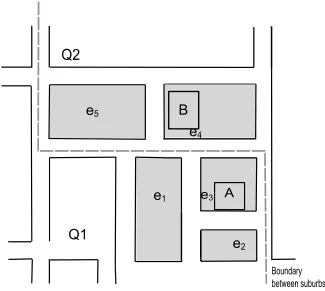
Fig. 7.Two suburbsQ1andQ2and their areas and specific buildings. The dashed line

4

Case study

We now present a case study that involves crowds of people that move in and between suburbs of a city and where the crowds can split and merge over time. Figure 7 shows a portion of the city where the action takes place. This example reflects the evolution of groups of people in a city during a demonstration. We assume that the entities to be modelled are groups of people, and that the identity and filiations of an entity are determined by the people that compose this group.

4.1 Overall Scenario

We consider the following four types of group which vary according to their behaviour and the distinction between these types would be significant in a surveillance operation. Different instances of these types arise for different values ofi.

• Ci: Demonstrators

• Wi: Pedestrians not involved in the demonstration

• Oi: Observers

• Gi: Unidentified people

We can record the filiation using the technique presented in [3] which distin-guishes between derivation and continuation. The case of continuation models the preservation of identity (such as an individual persisting throughout their life), and derivation models a new entity which depends in some manner on an earlier but distinct entity (for example a child could be modelled as a derived en-tity from each of their parents). We assume that filiation in the present scenario is determined as follows:

(1) If one or more people leave a groupX and join another groupZ, and/or if person(s) from another groupY join a groupX, then there are filiation links of type derivationδbetweenX andY, andX andZ. (Figure 8(a) and 8(b)) (2) Between two times, if a groupXremains the same without any addition/deletion

of people, it is considered in continuation relationγ. (Figure 8(c))

X

Z Y δ δ

(a)

X

Z Y

T δ δ δ (b)

X γ X

(c)

In the course of the demonstration, the different groups move around in the city. We suppose that the largest spatial unit we consider in the city is a suburb, and that there are two of these:Q1andQ2(Figure 7). Within suburbs there are areas determined by the street pattern and within some of these areas particular buildings have been identified as significant.

• Q1 contains three areas (e1,e2and e3) and a building Alocated ine3. • Q2 contains two areas (e4 ande5) and a building B located ate4.

4.2 Filiation Relations

Groups of people can may combine with each other, and they may divide into pieces. For example, the filiation relations shown in Figure 9 shows that a part of group C2 of demonstrators joins the group C1 to become G1. Groups are renamed when we consider that there is a change of their identity.

C1

C2

W1

W2

O1

O2

G1

G2

G3

W2

G4

O2

G1

G5

G3

G6

G9

G7

G8

G6

G9

t1 _H1 t2 H2 t3 H3 t4

δ δ δ

δ

γ δ

γ

γ

δ

γ

δ

δ δ δ

δ δ δ δ

γ

γ

Fig. 9.Filiation relationsH1 –H3between timest1–t4

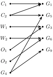
Between the four times t1 – t4 there are three relations H1 – H3. Using the cumulative product as described in section 2 we can computeH1⋆ H2, and this is illustrated in Figure 10. As the group G4 appears only at time t2 and is not present at t1 the cumulative product is able to record the fact that G5 andG9 have a common ancestor group. If we use the conventional composition

H1;H2 then this information, which could well be significant in a surveillance application, would not be available.

4.3 Bigraph modelling

trans-C1

C2

W1

W2

O1

O2

G4

G1

G5

G3

G6

G9

Fig. 10.Cumulative productH1⋆ H2 showing that common ancestry ofG9andG5 is

recorded whereas inH1;H2 it is forgotten

e1

e4

B

e3 A

e2

e5

Q1 Q1 Q1

Q1 Q1 Q1

Q1 Q1 Q1

Q2 Q2 Q2

Q2 Q2 Q2

Q2 Q2 Q2

O1

W1

W2 C1

C2

O2

e1

e4

B

e3 A

e2

e5

Q1 Q1 Q1

Q1 Q1 Q1

Q1 Q1 Q1

Q2 Q2 Q2

Q2 Q2 Q2

Q2 Q2 Q2

G9

G8

G7 G6

lated into the bigraph setting in Figures 12 and 13. In the first of these figures we provide the bigraph for the whole spatial area by presenting it as composite

S◦K1. This demonstrates another valuable feature of bigraphs as a spatial mod-elling tool: their ability to deal with spatial granularity. The bigraphSrepresents a low level of detail in which the two suburbs are distinguished but nothing is said about what may be found within them. The action of adding this detail and passing to the fully detailed descriptionS◦K1 corresponds precisely to the operation of composition for bigraphs.

As the change only affects a level of detail more specific than that modelled byS, we are able to show the changes at timest2–t4by just showing the bigraph which is composed with S. The three bigraphs we need are given in Figure 13. In these a link between two groups appears if there is a filiation between their ancestors. For example, at time t3, there is a filiation link between G9 andG5 because each contains some part ofG4. Similarly, the link betweenG1andG2at

t2leads to a link between G1 andG5 att3. Here G1 remains the same between these two times, andG2is only changed by the addition of people.

We have derived the bigraphs in Figures 12 and 13 by using the filiation data from Figure 9 and adding hypothetical spatial information. This approach means that we have treated each bigraph as a static snapshot of the situation at a given time, albeit a snapshot that contains some additional information about the ancestry of the groups present. This is certainly useful, but the full power of bigraphs only becomes apparent once we include rules as part of our modelling that specify how a bigraph at one stage may evolve into one at a subsequent stage. The introduction of rules is also significant in that by permitting only changes that are possible by given rules we can enforce integrity constraints in the model and ensure that semantically invalid changes are prohibited, such as moving one suburb inside another. In the next section we show how such rules can be introduced.

5

Bigraphs: Dynamic Aspects

5.1 Rewriting and Composition

We have seen that bigraphs represent spatial nesting and links. These links may be given several different interpretations, including channels of communication and records of communication having ocurred in the past. Both the place graph and the link graph can be subject to change, and in general these two features can change independently. To understand the mechanism of reaction rules, as they are called in the bigraph context, it may be helpful to consider the basic algebraic idea of rewrite rules.

An equation−(−x) =xmay be seen as a rewrite rule−(−x)_xallowing

O₁

W

1

W₂

Q₁ Q₂

C₁ A C₂ O₂ B e₂

e₁ e₃ e4 e₅

K

S

Fig. 12.Entire bigraph att1 is the CompositeS◦K1

G 6 G 9 G 1 A G 5 B e 2 e

1 e3

e

4 e₅ G 4 W 2 G 3 G 1 A G 2 O 2 B e 2 e

1 e3

e

4 e₅

A

B e

2 e

1 e3

e

4 e5 G 3 G 9 G 6 G 8 G 7

K

K

K

In expressing spatial dynamics with bigraphs a particular kind of change will consist of replacing one bigraph by another, just as we can replace−(−x) by xin the above example. The same kind of change may take place in many different contexts. In bigraphs this corresponds to the fact that ifH _K then

G◦H _ G◦K (assuming the composition is defined). Also the same kind of

change may be made more specific in many different ways, just as essentially the same change is happening in rewriting−(−(y+ 3)) toy+ 3 as in rewriting −(−(2y+ 2)) to 2y+ 2. This situation correponds to the fact that for bigraphs ifH _Kthen H◦G′_K◦G′ again assuming the composition is defined.

5.2 Rules for the Case Study

Here we present rules that enable the features of the case study to be modelled. To extract the most significant features of the case-study, we assume that there are just crowds of people without distinguishing different types. This restriction could be lifted by introducing a more elaborate signature, but would not involve any essentially different features of rules.

0

0

x

x

. . .

x

0

x

x

. . .

x

y

y

. . .

y

0

m

m+n

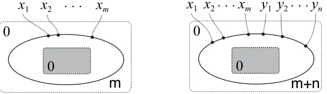
Fig. 14.The discrete ionsmx and (m+n)xy

For each crowd we are interested in what earlier groupings constitute the crowd. To formulate the rules we need to introduce some additional technicalities that were not necessary to convey the main ideas of the case study in the previous section. Milner [11, p30] uses the termdiscrete ion for a bigraph having a single node containing the single site of the bigraph, where also there are no inner names and the outer names are linked bijectively to the ports of the single node. Our signature has one type of node for each possible arity, where each port is capable of modelling a particular ancestor crowd. Thus a crowd constituted from three earlier ones needs three ports. This is illustrated in Figure 14 showing a discrete ion of aritymand typem_{. When the inner names arex}1, x2, . . . , xmwe

denote the ion by m_{x. To model the merging of two crowds, given for example}

inner namesx1, x2, . . . , xm, y1, y2, . . . , yn. We denote the type of such a node by

(m₊n_)xy.

In addition to the crowds, we need to model the buildings, areas and suburbs introduced in the case study. For these we use nodes of arity 0, since we do not model the historical development of these entities. The signature includes types

A_{for areas,}B_{for buildings and}S _{for subsurbs.}

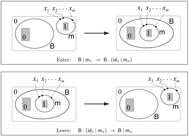
As a first example, the rules need to permit a crowd to enter, say, a building and to leave the building. This is straightforward, and is illustrated in Figure 15. The idea of entering or leaving a building is already well-known and appears as one of the motivating examples in [11]. However, the rules we present in Figures 16, and 17 represent a novel use of bigraphs in their use of links to model shared ancestry.

The two rules shown in Figure 16 allow one crowd to divide into two, and allow two crowds to merge into one. These can be used in cases such as the splitting ofG4 intoG5andG9 in our case study.

The rules shown in Figure 17 provide additional capabilities. These permit one crowd to surround another but to remain distinct. This could arise when a group of police surrounds a small crowd of deomstrators and forces them to move to another location, keeping them surrounded while moving. Although this behaviour is not illustrated by the case study, we include these rules as evidence of the power of bigraph rules to model more elaborate kinds of change.

0

0

1

x

x

. . .

x

m

B

0

0

1

x

x

. . .

x

m

B

Enter: B|mx _ B.(id1|mx)

0

0

1

x

x

. . .

x

m

B

0

0

1

x

x

. . .

x

m

B

Leave: B.(id1|mx) _ B|mx

0

x

x

. . .

x

1

0

0

0

1

x

x

. . .

x

m

m

m

Split: mx◦join _ mx|mx

0

x

x

. . .

x

y

y

. . .

y

1

0

0

0

1

x

x

. . .

x

y

y

. . .

y

m

n

m+n

Merge: mx|ny _ (m+n)_xy◦join

Fig. 16.Crowd Split and Merge Rules

0

x

x

. . .

x

y

y

. . .

y

1

2

0

1

2

0

x

x

. . .

x

y

y

. . .

y

0

m

n

m

n

_m

Capture: mx.(id1|ny|id1) _{_} mx.((ny.(mx|id1))|id1)

x

. . .

x

z

. . .

z

y

. . .

y

1

2

0

0

0

1

₂

x

. . .

x

z

. . .

z

y

. . .

y

0

m

n

_m+p

n

p

Release: mx.((ny.(pz|id1))|id1) _ (m+p)xz.(id1|ny|id1)

6

Conclusions and Further Work

We have given an expository account of the basic features of bigraphs and we have shown how a novel interpretation of the communication links as shared ancestry can be incorporated into models of spatio-temporal change. This inter-pretation is based on a way of combining relations, the cumulative product, that has advantages over the conventional composition operation. While this product is unlikely to be mathematically novel, we are not aware that it has been used before in the context of monitoring change in applications such as our case study. We have formulated bigraph reaction rules which can be used to model the splitting and merging of crowds of people and we have given further rules that model more elaborate behaviour including one group surrounding another so as to contain it.

Further work is necessary to analyse the theoretical properties of particular systems of rules. This could establish what kinds of spatio-temporal change are possible from particular rules. There will be close connections between the be-haviour of the split and merge rules for bigraphs and the splitting and merging studied in [9, 15]. There are also many possible application problems for spatio-temporal analysis described in the literature cited in the introduction. Further evaluation of the value of bigraphs needs to take place using some of these prob-lems. However, the evidence we have presented here demonstrates that bigraphs have several capabilities that are valuable in the modelling of spatio-temporal change.

References

1. Cohn, A.G., Renz, J.: Qualitative spatial representation and reasoning. In: van Harmelen, F., Lifschitz, V., Porter, B. (eds.) Handbook of knowledge representa-tion, pp. 551–596. Elsevier (2008)

2. Cressie, N., Wikle, C.K.: Statistics for Spatio-Temporal Data. John Wiley & Sons, Inc (2011)

3. Del Mondo, G., Stell, J., Claramunt, C., Thibaud, R.: A graph model for spatio-temporal evolution. Journal of Universal Computer Science 16(11), 1452–1477 (2010)

4. Duckham, M., Stell, J., Vasardani, M., Worboys, M.: Qualitative change to 3-valued regions. In: Fabrikant, S., et al. (eds.) Geographic Information Science, Lecture Notes in Computer Science, vol. 6292, pp. 249–263. Springer (2010) 5. Egenhofer, M.J., Franzosa, R.: Point-set topological spatial relations. International

Journal of Geographical Information Systems 5, 161–174 (1991) 6. Gallois, A.: Occasions of Identity. Clarendon Press, Oxford (1998)

7. Giudice, N.A., Walton, L.A., Worboys, M.: The informatics of indoor and outdoor space: A reasearch agenda. In: Winter, S., Jensen, C.S., Li, K.J. (eds.) Proceedings of the 2nd ACM SIGSPATIAL International Workshop on Indoor Spatial Aware-ness (ISA 2010). pp. 47–53. ACM Press (2010)

9. Jiang, J., Worboys, M.: Event-based topology for dynamic planar areal objects. International Journal of Geographical Information Science 23(1), 33–60 (2009) 10. Medak, D.: Lifestyles – An algebraic approach to change in identity. In: B¨ohlen,

M.H., Jensen, C.S., Scholl, M.O. (eds.) Spatio-Temporal Database Management. International Workshop STDBM’99. Proceedings. Lecture Notes in Computer Sci-ence, vol. 1678, pp. 19–38. Springer-Verlag (1999)

11. Milner, R.: The Space and Motion of Communicating Agents. Cambridge Univer-sity Press (2009)

12. O’Sullivan, D.: Geographical information science: time changes everything. Progress in Human Geography 29(6), 749–756 (2005)

13. Sevegnani, M., Calder, M.: Bigraphs with sharing. Tech. rep., University of Glas-gow, Department of Computing Science (2010)

14. Stell, J.: Granularity in change over time. In: Duckham, M., Goodchild, M., Wor-boys, M. (eds.) Foundations of Geographic Information Science, pp. 95–115. Taylor and Francis (2003)

15. Stell, J., Worboys, M.: Relations between adjacency trees. Theoretical Computer Science doi:10.1016/j.tcs.2011.04.029 (to appear 2011)

16. Walton, L., Worboys, M.: An algebraic approach to image schemas for geographic space. In: Stewart Hornsby, K., Claramunt, C., Denis, M., Ligozat, G. (eds.) Spa-tial Information Theory, 9th International Conference, COSIT 2009, Aber Wrac’h, France, September 21-25, 2009, Proceedings. Lecture Notes in Computer Science, vol. 5756, pp. 357–370. Springer (2009)

17. Williams, C.J.F.: What is Identity? Clarendon Press, Oxford (1989)