This is a repository copy of Approximate Bayesian computation (ABC) gives exact results under the assumption of model error.
White Rose Research Online URL for this paper: http://eprints.whiterose.ac.uk/99543/
Version: Accepted Version
Article:
Wilkinson, R.D. orcid.org/0000-0001-7729-7023 (2013) Approximate Bayesian
computation (ABC) gives exact results under the assumption of model error. Statistical Applications in Genetics and Molecular Biology, 12 (2). pp. 129-141. ISSN 2194-6302 https://doi.org/10.1515/sagmb-2013-0010
Reuse
Unless indicated otherwise, fulltext items are protected by copyright with all rights reserved. The copyright exception in section 29 of the Copyright, Designs and Patents Act 1988 allows the making of a single copy solely for the purpose of non-commercial research or private study within the limits of fair dealing. The publisher or other rights-holder may allow further reproduction and re-use of this version - refer to the White Rose Research Online record for this item. Where records identify the publisher as the copyright holder, users can verify any specific terms of use on the publisher’s website.
Takedown
If you consider content in White Rose Research Online to be in breach of UK law, please notify us by
arXiv:0811.3355v2 [stat.CO] 23 Apr 2013
Approximate Bayesian computation (ABC)
gives exact results under the assumption of
model error
Richard D. Wilkinson
∗School of Mathematical Sciences, University of Nottingham. NG7 2RD
[email protected]
April 24, 2013
Abstract
0-1 cut-off with an acceptance probability that varies with the distance of the simulated data from the observed data. The acceptance density gives the distribution of the error term, enabling the uniform error usually used to be replaced by a general distribution. This generalization can also be applied to approximate Markov chain Monte Carlo algorithms. In light of this work, ABC algorithms can be seen as calibration techniques for implicit stochas-tic models, inferring parameter values in light of the computer model, data, prior beliefs about the parameter values, and any measurement or model errors.
Keywords: Approximate Bayesian computation; calibration; implicit
infer-ence; likelihood-free inference.
1
Introduction
Approximate Bayesian computation (ABC) algorithms are a group of methods
for performing Bayesian inference without the need for explicit evaluation of the
model likelihood function (Beaumont et al., 2002, Marjoram et al., 2003, Sisson et al.,
2007). The algorithms can be used with implicit computer models (Diggle and Gratton,
1984) that generate sample data sets rather than return likelihoods. ABC methods
have become popular in the biological sciences (Sunnaker et al., 2013) with
ap-plications in genetics (see, for example, Siegmund et al., 2008, Foll et al., 2008),
epidemiology (Blum and Tran, 2010, Tanaka et al., 2006) and population biology
This popularity is primarily due to the fact that the likelihood function, which can
be difficult or impossible to compute for some models, is not needed in order to
do inference. However, despite their popularity little is known about the quality
of the approximation they provide beyond results shown in simulation studies.
In this paper we give a framework in which the accuracy of ABC methods can
be understood. The notation throughout this paper is as follows. Let θ denote
the vector of unknown model parameters we wish to infer, and letη(·)denote the
computer simulator. We assumeη(·)is stochastic, so that the simulator repeatedly
run atθ will give a range of possible outputs, and write X ∼η(θ)to denote that
X has the same distribution as the model run atθ. To distinguish the model output
from the observed data, let D denote the observations. The aim is to calibrate the
model to the data, in order to learn about the true value of the parameter. The
Bayesian approach is to find the posterior distribution ofθ given D, given by
π(θ |D) = π(D|θ)π(θ)
π(D) .
Throughout this paper, π(·)is used to denote different probability densities, and
π(· | ·) conditional densities, with the context clear from the arguments. Above,
π(θ) is the prior distribution, π(D|θ) is the likelihood of the data under the
model given parameter θ (the probability distribution of η(θ)), π(θ |D) is the
posterior distribution, andπ(D)is the evidence for the model.
It is usual in Bayesian inference to find that the normalizing constantπ(D)is
deal with this case (Liu, 2001). Doubly-intractable distributions are distributions
which have a likelihood functionπ(D|θ) =q(D|θ)/c(θ)which is known only up to a normalizing constant, c(θ), which is intractable. Standard Monte Carlo
techniques do not apply to these distributions, and Murray et al. (2006) have
de-veloped algorithms which can be used in this case. ABC methods are Monte Carlo
techniques developed for use with completely-intractable distributions, where the
likelihood function π(D| θ) is not even known up to a normalizing constant.
ABC algorithms, sometimes called likelihood-free algorithms, enable inference
using only simulations generated from the model, and do not require any
evalua-tion of the likelihood. The most basic form of the ABC algorithm is based on the
rejection algorithm, and is as follows:
Algorithm A: approximate rejection algorithm
A1 Drawθ ∼π(θ)
A2 Simulate X from the simulator X ∼η(θ)
A3 Accept θ ifρ(X,D)≤δ.
Here, ρ(·,·) is a distance measure on the model output space, and δ is a tol-erance determining the accuracy of the algorithm. Accepted values of θ are
not from the true posterior distribution, but from an approximation to it, written
π(θ |ρ(D,X)≤δ). Whenδ=0 this algorithm is exact and gives draws from the
posterior distributionπ(θ |D), whereas asδ →∞the algorithm gives draws from
the true posterior, they also lead to lower acceptance rates in step A3 than larger
values, and so more computation must be done to get a given sample size.
Con-sequently, the tolerance δ can be considered as controlling a trade-off between
computability and accuracy.
Several extensions have been made to the approximate rejection algorithm.
If the data are high dimensional, then a standard change to the algorithm is to
summarize the model output and data, using a summary statistic S(·)to project X
and D onto a lower dimensional space. Algorithm A is then changed so that step
A3 reads
A3′ Acceptθ ifρ(S(X),S(D))≤δ.
Ideally, S(·) should be chosen to be a sufficient statistic forθ. However, if the
likelihood is unknown, then sufficient statistics cannot be identified.
Summariz-ing the data and model output usSummariz-ing a non-sufficient summary adds another layer
of approximation on top of that added by the use of the distance measure and
tol-erance, but again, it is not known what effect any given choice for S(·)has on the
approximation.
In this paper it is shown that the basic approximate rejection algorithm can
be interpreted as performing exact inference in the presence of uniform model or
measurement error. In other words, it is shown that ABC gives exact inference for
the wrong model, and we give a distribution for the model error term for whatever
choice of metric and tolerance are used. This interpretation allows us to show
the effect a given choice of metric, tolerance and weighting have had in previous
in future work. It is also shown that Algorithm A can be generalized to give
inference under the assumption of a completely flexible form for the model error.
We discuss how to model the model error, and show how some models can be
rewritten to give exact inference. Ratmann et al. (2007) explored a related idea,
and looked at using ABC algorithms to diagnose model inadequacies. The aim
here is not to diagnose errors, but to account for them in the inference so as to
provide posteriors that take known inadequacies into account, and to understand
the effect of using standard ABC approaches.
Finally, ABC has been extended by Marjoram et al. (2003) from the
rejec-tion algorithm to approximate Markov chain Monte Carlo algorithms, and by
Sisson et al. (2007), Toni et al. (2009), and Beaumont et al. (2009) to approximate
sequential Monte Carlo algorithms. We extend the approximate Markov chain
Monte Carlo algorithm to give inference for a general form of error, and suggest
methods for calculating Bayes factors and integrals for completely-intractable
dis-tributions.
2
Interpreting ABC
In this section a framework is described which enables the effect a given metric
and weighting have in ABC algorithms to be understood. This will then allow
us to improve the inference by carefully choosing a metric and weighting which
more closely represents our true beliefs. The key idea is to assume that there
discrepancy represents either measurement error on the data, or model error
de-scribing our statistical beliefs about where the model is wrong. George Box
fa-mously wrote that ‘all models are wrong, but some are useful’, and in order to link
models to reality it is necessary to account for this model error when performing
inference. In the context of deterministic models, this practice is well established
(Campbell, 2006, Goldstein and Rougier, 2009, Higdon et al., 2008), and should
also be undertaken when linking stochastic models to reality, despite the fact that
the variability in the model can seemingly explain the data as they are.
The framework introduced here uses the best input approach, similar to that
given in Kennedy and O’Hagan (2001). We assume that the measurement D can
be considered as a realization of the model run at its best input value, ˆθ, plus an
independent error termε
D=η(θˆ) +ε. (1)
The error ε might represent measurement error on D, or model error in η(·),
or both, in which case we write ε =ε1+ε2. Discussion about the validity of
Equation (1), and whatε represents and how to model it are delayed until Section
3, and for the time being we simply considerε to have densityπε(·). The aim is
to describe our posterior beliefs about the best input ˆθ in light of the errorε, the
data D, and prior beliefs about ˆθ. Consider the following algorithm:
Algorithm B: probabilistic approximate rejection algorithm
B1 Drawθ ∼π(θ)
B3 Acceptθ with probability πε(Dc−X).
Here, c is a constant chosen to guarantee that πε(D−X)/c defines a probability.
For most cases we will expect ε to have a modal value of 0, and so taking c=
πε(0)will make the algorithm valid and also ensure efficiency by maximizing the
acceptance rate. If summaries are involved, or if D and X live in non-comparable
spaces, so that D−X does not make sense, we can instead use any distribution
relating X to D,πε(D|X)instead.
The main innovation in this paper is to show that Algorithm B gives exact
inference for the statistical model described above by Equation (1). This is
essen-tially saying that ABC gives exact inference, but for the wrong model.
Theorem 1 Algorithm B gives draws from the posterior distributionπ(θˆ|D) un-der the assumption that D=η(θˆ) +ε andε ∼πε(·)independently ofη(θˆ).
Proof 1 Let
I=
1 ifθ is accepted
0 otherwise.
We then find that
pr(I=1|θ) = Z
pr(I=1|η(θ) =x,θ)π(x|θ)dx
=
Z π
ε(D−x)
This gives that the distribution of accepted values ofθ is
π(θ |I=1) = π(θ) R
πε(D−x)π(x|θ)dx
R
π(θ′)R
πε(D−x)π(x|θ′)dxdθ′.
To complete the proof we must find the posterior distribution of the best model
input ˆθ given the data D under the assumption of model error. Note thatπ(D|
η(θˆ) =x) =πε(D−x)which implies that the likelihood ofθ is
π(D|θˆ) = Z
π(D|η(θˆ) =x,θˆ)π(x|θˆ)dx
= Z
πε(D−x)π(x|θˆ)dx.
Consequently, the posterior distribution of ˆθ is
π(θˆ |D) = π(θˆ) R
πε(D−x)π(x|θˆ)dx
R
π(θ)R
πε(D−x)π(x|θ)dxdθ
which matches the distribution of accepted values from Algorithm B.
To illustrate the algorithm, we consider the toy example used in Sisson et al.
(2007) and again in Beaumont et al. (2009) where analytic expressions can be
calculated for the approximations.
Example 1 Assume the model is a mixture of two normal distributions with a
uniform prior for the mean:
η(θ)∼1
2N (θ,1) + 1 2N (θ,
1
Further assume that we observe D=0, but that there is measurement errorε on
this data. Ifε∼U[−δ,δ], which is the assumption made when using Algorithm
A withρ(x,0) =|x|, then it is possible to show that the approximation is
π(θ|ε∼U[−δ,δ],D=0)∝ Φ(δ−θ)−Φ(−δ−θ)+Φ(10(δ−θ))−Φ(−10(δ+θ))
for θ ∈[−10,10], where Φ(·) is the standard Gaussian cumulative distribution function. An alternative to assuming uniform error, is to suppose that the error
has a normal distributionε∼N (0,δ2/3). It can then be shown that the posterior
distribution ofθ is
π(θ |ε∼N (0,δ 2
3 ),D=0)∝ 1
2φ(θ; 0,1+
δ2 3 ) +
1
2φ(θ; 0, 1 100+
δ2 3 )
truncated onto[−10,10]. This is the approximation found when using Algorithm B with a Gaussian acceptance kernel, whereφ(·;µ,σ2)is the probability density function of a Gaussian distribution with mean µ and varianceσ2. The value of
the variance, δ2/3, is chosen to be equal to the variance of a U[−δ,δ] random
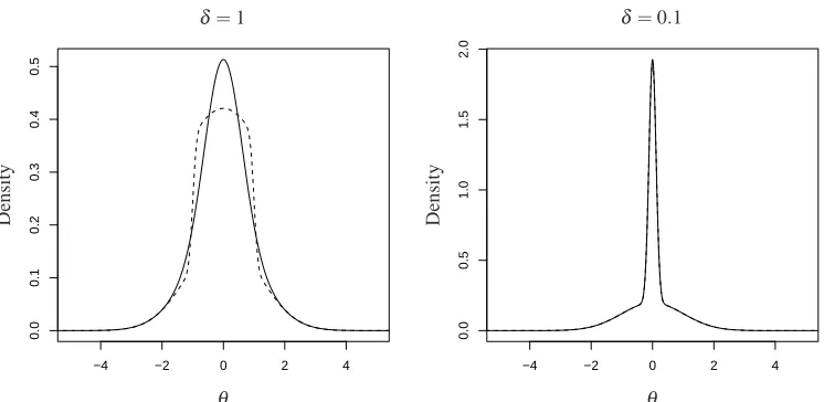
variable. For large values of the tolerance δ, the difference between the two
approximations can be significant (see Figure 1), but in the limit as δ tends to
−4 −2 0 2 4 0.0 0.1 0.2 0.3 0.4 0.5
−4 −2 0 2 4
0.0 0.5 1.0 1.5 2.0 D en si ty D en si ty θ θ
[image:12.612.114.487.133.315.2]δ=0.1 δ=1
Figure 1: The posterior distributions found when using Algorithm A (solid line) and Algorithm B (dashed line) with a Gaussian acceptance kernel. The left plot is forδ =1 and the right plot forδ =0.1. The two curves are indistinguishable in the second plot.
3
Model discrepancy
The interpretation of ABC given by Theorem 1 allows us to revisit previous
anal-yses done using the ABC algorithm, and to understand the approximation in the
posterior in terms of the distribution implicitly assumed for the error term. If the
approximate rejection algorithm (Algorithm A) was used to do the analysis, we
can see that this is equivalent to using the acceptance probability
πε(r)
c =
1 ifρ(r)≤δ
where r is the distance between the simulated and observed data. This says that
Algorithm A gives exact inference for the model which assumes a uniform
mea-surement error on the region defined by the 0-1 cut-off, i.e.,
ε∼U{x :ρ(x,D)≤δ}.
If ρ(·,·)is a Euclidean metric, ρ(D,x) = (x−D)T(x−D), this is equivalent to assuming uniform measurement error on a ball of radius δ about D. In most
situations, it is likely to be a poor choice for a model of the measurement error,
because the tails of the distribution are short, with zero mass outside of the interval
[−δ,δ].
There are two ways we can choose to view the error term; either as
mea-surement error or model error. Interpreting ε to represent measurement error is
relatively straight forward, as scientists usually hold beliefs about the distribution
and magnitude of measurement error on their data. For most problems,
assump-tions of uniform measurement error will be inappropriate, and so using Algorithm
A with a 0-1 cut-off will be inappropriate. But we have shown how to replace this
uniform assumption with a distribution which more closely represents the beliefs
of the scientist. Although the distribution of the measurement error will often be
completely specified by the scientist, for example zero-mean Gaussian error with
known variance, it is possible to include unknown parameters for the distribution
ofεinθ and infer them along with the model parameters. Care needs to be taken
all values of the parameter, but other than this it is in theory simple to infer error
parameters along with the model parameters. So for example, if ε ∼N (0,σ2), whereσ2is unknown, we could includeσ2inθ.
Some models have sampling or measurement error built into the computer
code so that the model output includes a realization of this noise. Rather than
coding the noise process into the model, it will sometimes be possible to rewrite
the model so that it outputs the latent underlying signal. If the likelihood of the
data given the latent signal is computable (as it often is), then it may be possible
to analytically account for the noise with the acceptance probabilityπε(·). ABC
methods have proven most popular in fields such as genetics, epidemiology, and
population biology, where a common occurrence is to have data generated by
sampling a hidden underlying tree structure. In many cases, it is the partially
observed tree structure which causes the likelihood to be intractable, and given
the underlying tree the sampling process will have a known distribution. If this
is the case (and if computational constraints allow), we can use the probabilistic
ABC algorithm to do the sampling to give exact inference without any assumption
of model error. Note that if the sampling process gives continuous data, then exact
inference using the rejection algorithm would not be possible, and so this approach
has the potential to give a significant improvement over current methods.
Example 2 To illustrate the idea of rewriting the model in order to do analytic
sampling, we describe a version of the problem considered in Plagnol and Tavar´e
(2004) and Wilkinson and Tavar´e (2009). Their aim was to use the primate fossil
branching process to model speciation, with trees rooted at time t=τ, and
simu-lated forwards in time to time t =0, so that the depth of the tree,τ, represents the
divergence time of interest. The branching process is parametrized by λ, which
can either be estimated and fixed, or treated as unknown and given a prior
dis-tribution. Time is split into geologic epochs τ <tk <· · ·<t1<0, and the data
consist of counts of the number of primate species that have been found in each
epoch of the fossil record, D= (D1, . . . ,Dk). Fossil finds are modelled by a
dis-crete marking process on the tree, with each species having equal probabilityα
of being preserved as a fossil in the record. If we let Nibe the cumulative number
of branches that exist during any point of epoch i, then the model used for the
fossil finds process can be written as Di∼Binomial(Ni,α). The distribution of
N = (N1, . . .,N14) cannot be calculated explicitly and so we cannot use a
likeli-hood based approach to find the posterior distribution of the unknown parameter
θ = (λ,τ,α). The ABC approach used in Plagnol and Tavar´e (2004) was to draw
a value ofθ from its prior, simulate a sample tree and fossil finds, and then count
the number of simulated fossils in each epoch to find a simulated value of the
data X . They then accepted θ if ρ(D,X)≤δ for some metric ρ(·,·) and toler-anceδ. This gives an approximation to the posterior distribution of the parameter
given the data and the model, where the approximation can be viewed as model
or measurement error.
However, instead of approximating the posterior, it is possible in theory to
rewrite the model and perform the sampling analytically to find the exact posterior
1. Drawθ = (λ,p,α)∼π(·)
2. Simulate a treeT using parameterλ and count N
3. Acceptθ with probability∏ki=1 Ni
Di
αDi(1−α)Ni−Di.
This algorithm gives exact draws from the posterior distribution ofθ given D, and
in theory there is no need for any assumption of measurement error. Note that θ
can include parameterα for the sampling rate, to be inferred along with the other
model parameters. However, this makes finding a normalizing constant in step 3
difficult. Without a normalizing constant to increase the acceptance rate, applying
this algorithm directly will be slow for many values of D and k (the choice of prior
distribution and number of parameters we choose to include inθ can also have a
significant effect on the efficiency). A practical solution would be to add an error
term and assume the presence of measurement error on the data (which is likely
to exist in this case), in order to increase the acceptance probability in step 3.
Approaching the problem in this way, it is possible to carefully model the error on
D and improve the estimate of the divergence time.
Usingε to represent measurement error is straight forward, whereas usingεto
model the model discrepancy (to account for the fact the model is wrong) is harder
to conceptualize and not as commonly used. For deterministic models, the idea
of using a model error term when doing calibration or data assimilation is well
established and described for a Bayesian framework in Kennedy and O’Hagan
(2001). They assume that the model run at its ‘best’ input, η(θˆ), is sufficient
at its best input provides all the available information about the system for the
purpose of prediction. If this is the case, then we can defineε to be the difference
betweenη(θˆ) and D, and assumeε is independent of η(θˆ). Note that the error
is the difference between the data and the model run at its best input, and does
not depend on θ. If we do not include an error termε, then the best input is the
value ofθ that best explains the data, given the model. When we include an error
term which is carefully modelled and represents our beliefs about the discrepancy
betweenη(·)and reality, then it can be argued that ˆθ represents the ‘true’ value of
θ, and thatπ(θˆ |D,ε∼πε(·))should be our posterior distribution for ˆθ in light
of the data and the model.
For deterministic models, Goldstein and Rougier (2009) provide a framework
to help think about the model discrepancy. To specify the distribution of ε, it
can help to break the discrepancy down into various parts: physical processes not
modelled, errors in the specification of the model, imperfect implementation etc.
So for example, ifη(·)represents a global climate model predicting average
tem-peratures, then common model errors could be not including processes such as
clouds, CO2 emissions from vegetation etc., error in the specification might be
using an unduly simple model of economic activity, and imperfect
implementa-tion would include using grid cells too large to accurately solve the underlying
differential equations. In some cases it may be necessary to consider model and
measurement error, ε+e say, and model each process separately. For stochastic
models, as far as we are aware, no guidance exists about how to model the error,
To complicate matters further, for many models the dimension of D and X
will be large, making it likely that the acceptance rate πε(X−D) will be small.
As noted above, in this case it is necessary to summarize the model output and
the data using a multidimensional summary S(·). Using a summary means that
rather than approximatingπ(θ |D), the algorithms approximateπ(θ |S(D)). The
interpretation ofε as model or measurement error still holds, but now the error is
on the measurement S(D)or the model prediction S(X). If each element of S(·)
has an interpretation in terms of a physical process, this may make it easier to
break the error down into independent components. For example, suppose that we
use S(x) = (x¯,sxx), the sample mean and variance of X , and that we then use the following acceptance density
πε(S(X)−S(D)) =π1(X¯−D¯)π2(sX X−sDD).
This is equivalent to assuming that there are two sources of model error. Firstly,
the mean prediction is assumed to be wrong, with the error distributed with
den-sityπ1(·). Secondly, it assumes that the model prediction of the variance is wrong,
with the error having distributionπ2(·). It also assumes that the error in the mean
prediction is independent of the error in the variance prediction. This
indepen-dence is not necessary, but helps with visualization and elicitation. For this reason
it can be helpful to choose the different components of S(·)so that they are close to
independent (independence may also help increase the acceptance rate). Another
is large) to find a smaller number of uncorrelated summaries of the data which
may have meaningful interpretations. In general however, it is not known how
to choose good summaries. Joyce and Marjoram (2008) have suggested a method
for selecting between different summaries and for deciding how many summaries
it is optimal to include. However, more work is required to find summaries which
are informative, interpretable and for which we can describe the model error.
Finally, once we have specified a distribution forε, we may find the acceptance
rate is too small to be practicable and that it is necessary to compromise (as in
Example 2 above). A pragmatic way to increase the acceptance rate is to use
a more disperse distribution for ε. This moves us from the realm of using ε to
model an error we believe exists, to using it to approximate the true posterior.
This is currently how most ABC methods are used. However, even when making
a pragmatic compromise, the interpretation of the approximation in terms of an
error will allow us to think more carefully about how to choose between different
compromise solutions.
Example 3 One of the first uses of an ABC algorithm was by Pritchard et al.
(1999), who used a simple stochastic model to study the demographic history of
the Y chromosome, and used an approximate rejection algorithm to infer
muta-tion and demographic parameters for their model. Their data consisted of 445 Y
chromosomes sampled at eight different loci from a mixture of populations from
around the world, which they summarized by just three statistics: the mean (across
for their sample was D≡(V,H,N)T = (1.149,0.6358,316)T. They elicited prior
distributions for the mutation rates from the literature, and used diffuse priors
for population parameters such as the growth rate and the effective number of
ancestral Y chromosomes. Population growth was modelled using a standard
co-alescent model growing at an exponential rate from a constant ancestral level,
and various different mutation models were used to simulate sample values for
the three summaries measured in the data. They then applied Algorithm A using
the metric
ρ(D,X) = 3
∏
i=1
Di−Xi
Di
(2)
where X is a triplet of simulated values for the three summaries statistics. They
used a tolerance value ofδ=0.1, which for their choice of metric corresponds to
an error of 10% on each measurement. This gives results equivalent to assuming
that there is independent uniform measurement error on the three data summaries,
so that the true values of the three summaries have the following distributions
V ∼U[1.0341,1.2624],H∼U[0.58122,0.71038],N∼U[284,348].
Beaumont et al. (2002) used the same model and data set to compare the relative
performance of Algorithm A with an algorithm similar to Algorithm B, using an
Epanechnikov density applied to the metric value (2) for the acceptance
probabil-ity πε(·). They set a value of δ (the cut-off in Algorithm A and the range of the
support forε in Algorithm B) by using a quantile Pδ of the empirical distribution
model runs with values closest to D. They concluded that Algorithm B gives more
accurate results than Algorithm A, meaning that the distribution found using
Al-gorithm B is closer to the posterior found when assuming no measurement error
(δ =0).
The conclusion that Algorithm B is preferable to Algorithm A for this model
is perhaps not surprising in light of what we now know, as it was not taken into
account that both algorithms used the same value of δ. For Algorithm A this
corresponds to assuming a measurement error with varianceδ2/3, whereas using
an Epanechnikov acceptance probability is equivalent to assuming a measurement
error with varianceδ2/5. Therefore, using Algorithm B uses measurement error
only 60% as variable as that assumed in Algorithm A, and so it is perhaps not
surprising that Algorithm B gives more accurate results in this case.
4
Approximate Markov chain Monte Carlo
For problems which have a tightly constrained posterior distribution (relative to
the prior), repeatedly drawing independent values ofθ from its prior distribution
in the rejection algorithm can be inefficient. For problems with a high dimensional
θ this inefficiency is likely to make the application of a rejection type algorithm
impracticable. The idea behind Markov chain Monte Carlo (MCMC) is to build
a Markov chain on θ and correlate successive observations so that more time is
spent in regions of high posterior probability. Most MCMC algorithms, such as
func-tion which we have assumed is not known. Marjoram et al. (2003) give an
ap-proximate version of the Metropolis-Hastings algorithm, which apap-proximates the
acceptance probability by using simulated model output with a metric and a 0-1
cut-off to approximate the likelihood ratio. This, as before, is equivalent to
as-suming uniform error on a set defined by the metric and the tolerance. As above,
this algorithm can be generalized from assuming uniform measurement error to
an arbitrary error term. Below, are two different algorithms to perform MCMC for
the model described by Equation (1). The difference between the two algorithms
is in the choice of sample space used to construct the stationary distribution. In
Algorithm C we consider the state variable to belong to the space of parameter
values Θ, and construct a Markov chain {θ1,θ2, . . .} which obeys the following dynamics:
Algorithm C: probabilistic approximate MCMC 1
C1 At time t, propose a move from θt to θ′ according to transition kernel
q(θt,θ′).
C2 Simulate X′∼η(θ′).
C3 Setθt+1=θ′with probability
r(θt,θ′|X′) = πε
(D−X′)
c min
1,q(θ
′,θ
t)π(θ′)
q(θt,θ′)π(θt)
, (3)
An alternative approach is to introduce the value of the simulated output as an
auxiliary variable and construct the Markov chain on the spaceΘ×X, whereX
is the space of model outputs.
Algorithm D: probabilistic approximate MCMC 2
D1 At time t, propose a move fromψt= (θt,Xt)toψ′= (θ′,X′)withθ′drawn from transition kernel q(θt,θ′), and X′simulated from the model usingθ′:
X′∼η(θ′)
D2 Setψt+1= (θ′,X′)with probability
r((θt,Xt),(θ′,X′)) =min
1,πε(D−X
′)q(θ′,θ
t)π(θ′)
πε(D−Xt)q(θt,θ′)π(θt)
, (4)
otherwise setψt+1=ψt.
Proof 2 (of convergence) To show that these Markov chains converge to the
re-quired posterior distribution, it is sufficient to show that the chains satisfy the
detailed balance equations
π(s)p(s,t) =π(t)p(t,s) for all s,t
For Algorithm C the transition kernel is the product of q(θ,θ′) and the ac-ceptance rate. To calculate the acac-ceptance rate, note that in Equation (3) the
acceptance probability is conditioned upon knowledge of X′and so we must
inte-grate out X′to find r(θ,θ′). This gives the transition kernel for the chain:
p(θt,θ′) =q(θt,θ′)
Z
X
πε(D−X′)
c min
1,q(θ
′,θ
t)π(θ′)
q(θt,θ′)π(θt)
π(X′|θ′)dX′.
The target stationary distribution is
π(θ |D) = π(θ) R
X πε(D−X)π(X|θ)dX
π(D) .
It is then simple to show that the Markov chain described by Algorithm C satisfies
the detailed balance equations (see Liu (2001) for comparable calculations).
For Algorithm D, the transition kernel is
p((θt,Xt),(θ′,X′)) =q(θt,θ′)π(X′|θ′)min
1,πε(D−X
′)q(θ′,θ
t)π(θ′)
πε(D−Xt)q(θt,θ′)π(θt)
.
(5)
The Markov chain in this case takes values inΘ×X and the required stationary
distribution is
π(θ,X|D) = πε(D−X)π(X |θ)π(θ)
π(D) . (6)
It can then be shown that Equations (5) and (6) satisfy the detailed balance
While Algorithm C is more recognisable as a generalization of the approximate
MCMC algorithm given in Marjoram et al. (2003), Algorithm D is likely to be
more efficient in most cases. This is because the ratio of model error densities that
occurs in acceptance rate (4) is likely to result in larger probabilities than those
given by Equation (3) which simply has aπε(D−x)/c term instead. Algorithm D
also has the advantage of not requiring a normalizing constant.
5
Extensions
5.1
Importance sampling
Suppose our aim is to calculate expectations of the form
E(f(θ)|D) = Z
f(θ)π(θ |D)dθ
where the expectation is taken with respect to the posterior distribution ofθ. The
simplest way to approximate this is to draw a sample of θ values {θi}i=1,...,n,
from π(θ |D) using Algorithm B, C or D and then approximate using the sum
n−1∑f(θi). However, a more stable estimator can be obtained by using draws
from the prior weighted by πε(D−Xi) as in Algorithm B. For each(θi,Xi)pair drawn from the prior and simulator in steps B1 and B2, assign θi weight wi=
πε(D−Xi). Then an estimator of the required expectation is
∑f(θi)wi
This is an importance sampling algorithm targeting the joint distribution
π(X,θ |D)∝πε(D−X)π(X |θ)π(θ)
using instrumental distributionπ(X|θ)π(θ). Note that if the uniform acceptance
kernel
πε(D−X)∝Iρ(D,X)≤δ
is used, then this approach reduces to the rejection algorithm, as proposals are
given weight 1 (accepted) or 0 (rejected), showing that there is no uniform-ABC
version of importance sampling.
Sequential Monte Carlo algorithms are possible however, and Sisson et al.
(2007) and Toni et al. (2009) considered algorithms in which the tolerance δ is
slowly reduced through a schedule δ1, . . . ,δT to some small final value. Both of these algorithms, as well as variants such as Drovandi et al. (2011) and Del Moral et al.
(2012), which use Metropolis-Hastings moves of the parameter between iterations
to provide more efficient proposals, can be extended to the generalised ABC case
using general acceptance kernels. The move from 0-1 cut-offs to general
accep-tance rates can introduce difficulties with memory constraints, due to the
require-ment to store a large number of particles, many with small but non-zero weights.
Partial rejection control, introduced by Liu (2001) and extended to an ABC
set-ting by Peters et al. (2012), can be used to reject particles with small weights, only
5.2
Model selection
The theoretical acceptance rate from the rejection algorithm (Algorithm A with
δ =0) is equal to the model evidenceπ(D). The evidence from different models
can then be used to calculate Bayes factors which can be used to perform model
selection (Kass and Raftery, 1995). It is possible to approximate the value ofπ(D)
by using the acceptance rate from Algorithm A (Wilkinson, 2007). By doing this
for two or more competing models, we can perform approximate model
selec-tion, although in practice this approach can be unstable as δ varies (Wilkinson,
2007). The estimate of π(D) can be improved and made interpretable by using
the weighted estimate
1
n
n
∑
i=1 1
m
m
∑
j=1
πε(D−Xij)
where Xi1, . . . ,Xim∼η(θi)andθ1, . . . ,θn∼π(·). This gives a more stable estima-tor than simply taking the acceptance rate, and also tends to the exact value (as
n,m→∞) for the model given by Equation (1).
Robert et al. (2011) and Didelot et al. (2011) have highlighted the dangers of
using ABC algorithms for model selection when D and X are replaced by
sum-maries S(D)and S(X). The Bayes factor based on the full data D, will in general
differ from the Bayes factor based on the summary S(D), even when S is a
suffi-cient statistic forθ for both simulators.
The approach advocated here, of considering ABC as an extension of the
modelling process, using acceptance kernel πε(D−X) (or πε(S(D)|S(X)) in a
simula-tor output and observations (as encapsulated by Theorem 1), suggests a different
approach. The choice of acceptance kernel should be made after careful
consid-eration of the simulator’s ability, and inevitably involves a degree of subjective
judgement (as does the choice of simulator, prior, and summary statistics). The
kernel used forms part of the statistical model, and any model selection scheme
will assess this choice, as well as the choice of simulator and prior. In other words,
it is inevitable that the estimated Bayes factor will depend uponπε in general,
fur-ther highlighting the need for its careful design.
Similarly, the choice of summary statistic S(D)used to reduce the dimension
of the data and simulator output, should be based on careful consideration of what
aspects of the data we expect the simulator to be able to reproduce. Recent work
by Nunes and Balding (2010), Fearnhead and Prangle (2012), Barnes et al. (2012)
and Prangle et al. (2013) has focussed on automated methods for choosing good
summary statistics, but care should be taken to ensure the summaries selected
coincide with the modeller’s expectations of what the simulator can reproduce.
Examples can be constructed in which summaries are strongly informative about
the parameters (in the sense of π(θ|S(D)) differing from π(θ)), but which do
not produce believable posteriors. For example, in dynamical system models,
phase sensitive summaries (such as the sum of square differences) are usually
in-formative about the simulator parameters, even though the simulators were only
designed to capture the phase-insensitive parts of the system. Using these
sum-maries will give the appearance of having learned about the parameters, as the
is of value. If the summary S(D) is chosen on a sound physical basis, and the
inference viewed as conditional upon this choice (i.e., the posterior is taken to
be π(θ|S(D))and is not seen as an approximation to π(θ|D)), then the
difficul-ties for ABC model selection raised by Robert et al. (2011) are circumvented, and
interpretation is clear.
6
Discussion
It has been shown in this paper that approximate Bayesian computation algorithms
can be considered to give exact inference under the assumption of model error.
However, this is only part of the way towards a complete understanding of ABC
algorithms. In the majority of the application papers using ABC methods,
sum-maries of the data and model output have been used to reduce the dimension of
the output. It cannot be known whether these summaries are sufficient for the
data, and so in most cases the use of summaries means that there is another layer
of approximation. While this work allows us to understand the error assumed
on the measurement of the summary, it says nothing about what effect using the
summary rather than the complete data has on the inference.
The use of a simulator discrepancy term when making inferences is important
if one wants to move from making statements about the simulator to statements
about reality. There has currently been only minimal work done on modelling the
discrepancy term for stochastic models. One way to approach this is to view the
(many realizations of η(θ) would be needed to learn πθ(x)). The discrepancy
term ε can then be considered as representing the difference between πθ(x)and
the true variability inherent in the physical system.
Acknowledgements
I would like to thank Professor Paul Blackwell for his suggestion that the metric in
the ABC algorithm might have a probabilistic interpretation. I would also like to
thank Professor Simon Tavar´e, Professor Tony O’Hagan, and Dr Jeremy Oakley
for useful discussions on an early draft of the manuscript.
References
Barnes, C. P., Filippi, S., Stumpf, M. P. H., Thorne, T., 2012. Considerate
ap-proaches to achieving sufficiency for ABC model selection. Stat. Comput. 22,
1181–1197.
Beaumont, M. A., Cornuet, J. M., Marin, J. M., Robert, C. P., 2009. Adaptivity
for ABC algorithms: the ABC-PMC. Biometrika 96 (4), 983–990.
Beaumont, M. A., Zhang, W., Balding, D. J., 2002. Approximate Bayesian
com-putatation in population genetics. Genetics 162 (4), 2025–2035.
Blum, M., Tran, V., 2010. HIV with contact tracing: a case study in approximate
Campbell, K., 2006. Statistical calibration of computer simulations. Reliab. Eng.
Syst. Safe. 91, 1358–1363.
Cornuet, J.-M., Santos, F., Beaumont, M. A., Robert, C. P., Marin, J.-M., Balding,
D. J., Guillemaud, T., Estoup, A., 2008. Inferring population history with DIY
ABC: a user-friendly approach to approximate Bayesian computation.
Bioin-formatics 24 (23), 2713–2719.
Del Moral, P., Doucet, A., Jasra, A., 2012. An adaptive sequential Monte Carlo
method for approximate Bayesian computation. Stat. Comput. 22, 1009–1020.
Didelot, X., Everitt, R. G., Johansen, A. M., Lawson, D. J., 2011. Likelihood-free
estimation of model evidence. Bayesian analysis 6, 49–76.
Diggle, P. J., Gratton, R. J., 1984. Monte Carlo methods of inference for implicit
statistical models. J. R. Statist. Soc. B 46 (2), 193–227.
Drovandi, C. C., Pettitt, A. N., Faddy, M. J., 2011. Approximate Bayesian
com-putation using indirect inference. J. Roy. Stat. Soc. Ser. C 60, 317–337.
Fearnhead, P., Prangle, D., 2012. Constructing summary statistics for approximate
Bayesian computation: semi-automatic approximate Bayesian computation. J.
Roy. Stat. Soc. Ser. B 74, 419–474.
Foll, M., Beaumont, M. A., Gaggiotti, O., 2008. An approximate Bayesian
com-putation approach to overcome biases that arise when using amplified fragment
Goldstein, M., Rougier, J., 2009. Reified Bayesian modelling and inference for
physical systems. J. Stat. Plan. Infer. 139 (3), 1221 – 1239.
Hamilton, G., Currat, M., Ray, N., Heckel, G., Beaumont, M. A., Excoffier, L.,
2005. Bayesian estimation of recent migration rates after a spatial expansion.
Genetics 170, 409–417.
Higdon, D., Gattiker, J., Williams, B., Rightley, M., 2008. Computer model
cali-bration using high-dimensional output. J. Am. Statis. Assoc. 103, 570–583.
Joyce, P., Marjoram, P., 2008. Approximately sufficient statistics and Bayesian
computation. Stat. Appl. Genet. Mo. B. 7 (1), article 26.
Kass, R. E., Raftery, A. E., 1995. Bayes factors. J. Am. Statis. Assoc. 90 (430),
773–795.
Kennedy, M., O’Hagan, A., 2001. Bayesian calibration of computer models (with
discussion). J. R. Statist. Soc. Ser. B 63, 425–464.
Liu, J. S., 2001. Monte Carlo Strategies in Scientific Computing. Springer Series
in Statistics. New York: Springer.
Marjoram, P., Molitor, J., Plagnol, V., Tavar´e, S., 2003. Markov chain Monte Carlo
without likelihoods. P. Natl. Acad. Sci. USA 100 (26), 15324–15328.
Murray, I., Ghahramani, Z., MacKay, D. J. C., 2006. MCMC for
doubly-intractable distributions. In: Proceedings of the 22nd Annual Conference on
Nunes, M. A., Balding, D. J., 2010. On optimal selection of summary statistics
for approximate Bayesian computation. Stat. Appl. Genet. Mo. B. 9, Article 34.
Peters, G., Fan, Y., Sisson, S., 2012. On sequential Monte Carlo, partial rejection
control and approximate Bayesian computation. Stat. Comput. 22, 1209–1222.
Plagnol, V., Tavar´e, S., 2004. Approximate Bayesian computation and MCMC.
In: Niederreiter, H. (Ed.), Proceedings of Monte Carlo and Quasi-Monte Carlo
Methods 2002. Springer-Verlag, pp. 99–114.
Prangle, D., Fearnhead, P., Cox, M. P., French, N. P., 2013. Semi-automatic
se-lection of summary statistics for abc model choice. In submission, available as
arXiv:1302:5624.
Pritchard, J. K., Seielstad, M. T., Perez-Lezaun, A., Feldman, M. W., 1999.
Popu-lation growth of human Y chromosomes: a study of Y chromosome
microsatel-lites. Mol. Biol. Evol. 16 (12), 1791–1798.
Ratmann, O., Jorgensen, O., Hinkley, T., Stumpf, M., Richardson, S., Wiuf, C.,
2007. Using likelihood-free inference to compare evolutionary dynamics of the
protein networks of H. pylori and P. falciparum. PLoS Comput. Biol. 3 (11),
2266–2276.
Robert, C. P., Cornuet, J. M., Marin, J. M., Pillai, N. S., 2011. Lack of confidence
in approximate Bayesian computation model choice. P. Natl. Acad. Sci. USA
Siegmund, K. D., Marjoram, P., Shibata, D., 2008. Modeling DNA methylation in
a population of cancer cells. Stat. Appl. Genet. Mo. B. 7 (1), article 18.
Sisson, S. A., Fan, Y., Tanaka, M. M., 2007. Sequential Monte Carlo without
likelihoods. Proc. Natl. Acad. Sci. USA 104 (6), 1760–1765.
Sunnaker, M., Busetto, A. G., Numminen, E., Corander, J., Foll, M., Dessimoz,
C., 2013. Approximate bayesian computation. PLoS Comput Biol 9, e1002803.
Tanaka, M. M., Francis, A. R., Luciani, F., Sisson, S. A., 2006. Using approximate
Bayesian computation to estimate tuberculosis transmission parameters from
genotype data. Genetics 173, 1511–1520.
Toni, T., Welch, D., Strelkowa, N., Ipsen, A., Stumpf, M. P. H., 2009.
Approxi-mate Bayesian Computation scheme for parameter inference and model
selec-tion in dynamical systems. J. R. Soc. Interface 6 (31), 187–202.
Wilkinson, R. D., 2007. Bayesian inference of primate divergence times. Ph.D.
thesis, University of Cambridge.
Wilkinson, R. D., Tavar´e, S., 2009. Estimating primate divergence times by using