City, University of London Institutional Repository
Citation
:
Zhao, X., Littlewood, B., Povyakalo, A. A. & Wright, D. (2015). Conservative
Claims about the Probability of Perfection of Software-based Systems. Paper presented at
the The 26th IEEE International Symposium on Software Reliability Engineering, 02-11-2015
- 05-11-2015, Washington DC, USA.
This is the accepted version of the paper.
This version of the publication may differ from the final published
version.
Permanent repository link:
http://openaccess.city.ac.uk/12803/
Link to published version
:
Copyright and reuse:
City Research Online aims to make research
outputs of City, University of London available to a wider audience.
Copyright and Moral Rights remain with the author(s) and/or copyright
holders. URLs from City Research Online may be freely distributed and
linked to.
City Research Online:
http://openaccess.city.ac.uk/
[email protected]
Conservative Claims about the Probability of
Perfection of Software-based Systems
Xingyu Zhao, Bev Littlewood,
Centre for Software Reliability,City University London, U.K. {Xingyu.Zhao.1, B.Littlewood}@city.ac.uk
Andrey Povyakalo, David Wright,
Centre for Software Reliability,City University London, U.K. {A.A.Povyakalo, D.R.Wright}@city.ac.uk
Abstract— In recent years we have become interested in the problem of assessing the probability of perfection of software-based systems which are sufficiently simple that they are “possibly perfect”. By “perfection” we mean that the software of interest will never fail in a specific operating environment. We can never be certain that it is perfect, so our interest lies in claims for its probability of perfection. Our approach is Bayesian: our aim is to model the changes to this probability of perfection as we see evidence of failure-free working. Much of the paper considers the difficult problem of expressing prior beliefs about the probability of failure on demand (pfd), and representing these mathematically. This requires the assessor to state his prior belief in perfection as a probability, and also to state what he believes are likely values of the pfd in the event that the system is not
perfect. We take the view that it will be impractical for an assessor to express these beliefs as a complete distribution for
pfd. Our approach to the problem has three threads. Firstly we assume that, although he cannot provide a full probabilistic description of his uncertainty in a single distribution, the assessor can express some precise but partialbeliefs about the unknowns. Secondly, we assume that in the inevitable presence of such incompleteness, the Bayesian analysis needs to provide results that are guaranteed to be conservative (because the analyses we have in mind relate to critical systems). Finally, we seek to prune the set of prior distributions that the assessor finds acceptable in order that the conservatism of the results is no greater than it has to be, i.e. we propose, and eliminate, sets of priors that would appear generally unreasonable. We give some illustrative numerical examples of this approach, and note that the numerical values obtained for the posterior probability of perfection in this way seem potentially useful (although we make no claims for the practical realism of the numbers we use). We also note that the general approach here to the problem of expressing and using limited prior belief in a Bayesian analysis may have wider applicability than to the problem we have addressed.
Keywords— Probability of perfection, conservative claims, reliability assessment, 1oo2 systems
I. INTRODUCTION: WHY “PROBABILITY OF PERFECTION”? Software-based systems are used in an increasing number of applications where their failures may be very costly, in terms of monetary loss or human suffering. As a result, such systems often have very high dependability requirements. For example, for flight-critical avionics systems in civil transport airplanes there is a requirement of less than 10-9 probability of
failure per hour of operation [1]. Some demand-based systems have similarly stringent requirements: e.g. the claimed probability of failure on demand (pfd) for the combined control and instrumentation safety systems on the UK European Pressurised Reactor (UK EPR) is 10-9 [2].
There are different reasons why such high reliabilities are needed. In the aircraft example, there will be massive exposure worldwide for a particular aircraft fleet, and thus for a critical flight-control system. For example, the Airbus A320 and its siblings had by 2013 experienced some 80m flight departures (with an average flight time of a little under two hours) [5]. Society demands that fatal accidents remain very infrequent, even as commercial flights increase in number. In the case of nuclear power reactors, exposure measured in operating hours will be much more modest, but worst case accidents may have catastrophically greater consequences and thus need to be extremely unlikely [16]. In many other industries – such as control of hazardous chemical plant – the safety and reliability requirements are similarly stringent.
To achieve these kinds of ultra-high reliabilities is clearly a difficult task of design and implementation. The problems of
assessing what has been achieved – so as to be sufficiently confident that a particular system is safe enough to use – seem to us to be even harder. Direct black-box operational testing, for example, would require infeasible times on test [3] to support claims for the failure rates, or pfds, needed in examples like the ones above1.
In this paper we consider a different approach to this difficult problem of assessment. The idea is that, instead of claims for reliability – failure rates, pfds, etc – we make claims for perfection. This word comes, we realise, with extensive baggage: here it just means that a “perfect” system will not fail however much operational exposure it receives. If we assume that failures of a software system can occur if and only if it contains faults, it means that the system is “fault-free”. Readers may think, reasonably, that we can never be certain that a system is perfect in this sense; but they may be prepared to accept that such perfection is possible. In the face of this uncertainty, we shall use “probability of perfection” as a measure of how good such a system is.
In fact, as John Rushby has pointed out [9, 15], the traditional processes of software assurance, such as those performed in support of DO-178B (the guidelines for the certification of safety-critical aircraft software), can be best understood as developing evidence of possible perfection, rather than ultra-high reliability. Indeed, claims for the perfection of some systems may be more intuitively plausible than claims for very high reliability, since the two would be based upon different types of evidence and reasoning. A claim for 10-9 probability of failure per hour seems to acknowledge that the system in question is unlikely to be perfect – for example because of the complexity of its functionality – and resulting assessment of an extremely small number may not be believable2. A claim for perfection, on the other hand, may be based upon evidence that the design is simple enough that the designers had a chance of “getting it right”.
Why should we seek to be confident that a software system is perfect, rather than reliable? What benefits does this change of view bring to the problem of assessing the safety of a wider system? There seem to be two ways in which this approach may make the system assessment problem easier. The first concerns the need to assess the chance of lifetime freedom from system failure; the second concerns the need to assess the reliability of multi-channel software-diverse fault tolerant systems, since these are obvious candidates for these demanding safety-critical roles (and have been demonstrated to be effective – after the fact – in some cases, e.g. some Airbus aircraft).
Consider first the problem of lifetime reliability of a critical on-demand3 system, such as a safety shut-down system for a nuclear reactor or hazardous chemical process. Whilst requirements of such a system are often expressed in terms of probability of failure on (a single) demand (pfd), in fact for most systems what is really needed is a high confidence that only a small number of failures will occur over all demands in the expected life of the system. For some systems – e.g. nuclear reactor protection systems – this number may be zero. A pfd claim is thus really in support of a lifetime claim.
The point here is that a probability of perfection directly addresses a lifetime claim: it is precisely the probability that the system will experience no failures, no matter how long its exposure (number of demands over its life) [12, 17]. Consider the following (artificial) example to illustrate this point. Let’s say we have a system for which we expect 100 demands in its lifetime, and we want to be 99% confident that it will survive all these without failure. To obtain such confidence, we need the pfd to be no worse than about 10-4. If we expected 1000 demands during its lifetime, we would need a pfd no worse than about 10-5 to be 99% confident of seeing no failures. For 10,000 demands, we need a
pfd of about 10-6, and so on. As the expected number of lifetime demands increases, the required pfd needed to be 99% confident of seeing no failures becomes more and more demanding. In contrast, of course, we could be 99% confident of seeing no failures in any
number of demands if we were 99% confident in perfection. If we could support such a possible perfection claim, the need for
2For example, in exceedingly long operational testing, doubts about the representativeness of the testing, and the correctness of the test oracle, may come to dominate.
3 We shall use the terminology of on-demand systems for the rest of the paper, but much of what we say will also be applicable to continuously operating systems.
extremely extensive (possibly infeeasibly so) testing to establish a very small pfd disappears4.
The second reason we might wish to claim a probability of perfection arises from some recent work on design diversity. Design diversity has been proposed as a promising way of achieving high dependability for software-based systems. The intuitive explanation is that if we force two or more systems to be built differently, their resulting failures may also be different. So if, in a 1-out-of-2 protection system (1oo2 system), channel A fails on a particular demand, there may be a good chance that channel B will not fail. There is evidence from some industrial applications that this kind of design diversity has been successful [4]. For example, the safety-critical flight control systems of Airbus fleets have experienced massive operational exposure [5] with apparently no critical failure.
Such evidence was, of course, only available after the fact. Assessing the reliability of such a design-diverse system before it is deployed remains a very difficult problem. We know, from experimental work [6, 7] and theoretical modelling [8] that we cannot claim with certainty that there is independence between the failures of multiple software-based channels of a system. Thus for a 1oo2 system, if channel A fails on a randomly selected demand, this may increase the likelihood that the demand is a “difficult” one and so increase the likelihood that channel B also will fail. So even if we know the marginal probabilities of failures of the two channels, say pfdA and pfdB, from extensive testing, we cannot simply multiply them and claim the system pfd is pfdA ×pfdB.
In recent work by Littlewood and Rushby [9], the authors proposed a new way to reason about the reliability of a special kind of 1oo2 systems. Here channel A is conventionally engineered and presumed to contain faults, and thus supports only a pfd claim (say pfdA). Channel B on the other hand is extremely simple and extensively analyzed, and thus is “possibly perfect”; in [9] the claim about this channel is a probability of non-perfection, pnpB5. Littlewood and Rushby show that:
Pr(system fails on randomly selected demand |pfdA,pnpB)
≤pfdA×pnpB
The result depends on the events “A fails on a randomly selected demand” and “B is not perfect” being conditionally independent, given that the probabilities of these events, respectively pfdA and pnpB, are known. This is a conservative bound for the system’s probability of failure on demand (pfdsys), and the conservatism arises by assuming that if B is imperfect, it always fails when A does. The result is useful because it allows multiplication of two small numbers to obtain (a bound on) pfdsys (cf the result above involving the product of the small numbers pfdA and pfdB, which requires the improbable assumption of independence of channel failures).
4 In this informal account, for simplicity, we have not taken account of the inevitable epistemic uncertainty about the values of the system pfd.
In reality, of course, an assessor would not know pfdA and
pnpB with certainty: there is epistemic uncertainty about their numerical values. In principle, an assessor could represent his uncertainty here via a (bivariate) distribution for the two unknowns. In practice people find this kind of thing very difficult, if not impossible. Whilst assessors may be able to make informed statements about their marginal beliefs about the two parameters separately, they will usually be unable to say anything about their dependence.
In [10], Littlewood and Povyakalo address this problem. They obtain results that require only an assessor’s marginal beliefs about the individual numbers, i.e. they do not require the assessor to say anything about dependence between the two numbers. The price paid here is further conservatism, in addition to that arising from the result of [9].
The results of [9] and [10], then, have reduced the problem of assessing the pfd of this kind of special 1oo2 system to one concerning simply marginal beliefs about the parameters pfdA and pnpB. There is a large literature on the assessment of pfd from statistical analysis of operational tests [11], so the first of these parameters could be easily assessed, e.g. in terms of a Bayesian posterior distribution. That leaves pnpB, which is the subject of the current paper.
The question about probability of perfection upon which we concentrate here is what can be claimed about it from seeing many failure-free tests. We develop a probability model for this problem, and illustrate it with some numerical examples. Much of the paper addresses some difficult issues of prior beliefs in the Bayesian framework: our approach is to support conservative claims for probability of perfection based on limited prior belief, but these should be no more conservative than is necessary. We argue that this general approach may have wider applicability than to the example considered here.
II. CLAIMS FOR PROBABILITY OF PERFECTION BASED ON FAILURE-FREE TESTING EVIDENCE
A. Informal introduction to our approach: the problem of the prior distribution
Our approach to the problem is similar to that we introduced in [13]. However, in that work our interest centered upon the problem of obtaining conservative claims for system
pfd; here our aim is to obtain conservative claims for probability of perfection (from which, of course, we can calculate a probability of non-perfection as required, for example, for the Littlewood/Rushby model).
We begin with an informal and intuitive explanation of our general approach, before giving an account of the modelling details.
We start by assuming that for every software-based system (or channel), there is a true unknown pfd, say P. As a thought experiment, we could imagine executing a large number of demands, n, selected in a way that accurately represents operational use, and allowing n to approach infinity: the proportion of failed demands would converge to the true (but unknown) pfd, P.
In practice, of course, there will only be a finite amount of evidence available, so the assessor will still be uncertain about the magnitude of the pfd after seeing this evidence. In the usual Bayesian terminology, this evidence will be used to update an assessor’s prior beliefs about the unknown pfd to obtain his posterior beliefs: Bayes’ Theorem modifies his uncertainty about the unknown pfd in the light of the evidence (but he does not arrive at certainty).
If an assessor were able to specify a complete distribution to represent his prior beliefs about the pfd, it is a simple matter to use Bayes’ Theorem to obtain his exact posterior distribution after he has seen the results. From this he could express his modified beliefs about quantities of interest such as the expected value of P (best “point” estimate), percentiles (confidence bounds for P), and so on.
A major – and often expressed – difficulty with the Bayesian approach is that assessors find it difficult, if not impossible, to express their prior uncertainty in terms of a complete probability distribution. This observation seems particularly pertinent for the kinds of software systems that are the subject of the present paper. In contrast to some other applications of Bayesian statistics (e.g. some medical scenarios), where there is extensive previous empirical evidence that can be used to inform an assessor’s prior judgments about this system, such evidence is often lacking, or very meagre, in software engineering applications. This is particularly true of safety critical applications.
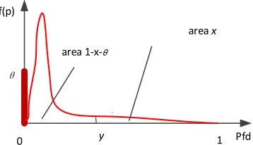
Our main purpose here, then, is to show some ways that this problem can be addressed when our interest centres on an assessor’s confidence in the perfection of a software system. In such a case, as we have said, the assessor cannot realistically be certain, a priori, that the system is perfect. Instead, he will have a prior probability of perfection, Pr(P=0)=θ. Since perfection is not certain, the assessor must in addition specify his prior beliefs about the possible non-zero values of the pfd. Ideally, then, he would be able to express his beliefs about the system pfd in terms of a complete distribution over the interval [0,1] that has probability mass at the origin: see Figure 1 for an idealized depiction of such a distribution. In the absence of such a complete prior distribution for the assessor’s prior beliefs, what can be said? Our approach to the problem is two-pronged.
Firstly, we recognize the reality that an assessor may only be able to express extremely limited beliefs about the likelihood of the pfd taking particular values in the interval. Specifically, we shall assume that he can only tell us a single percentile6 of the distribution of pfd, in addition to his expressed confidence in perfection. That is, he is only willing and/or able to express the following two precise beliefs:
θ = =0) (
Pr P (1)
θ − − = < <P y) 1 x 0
(
Pr (2)
where he states the values 0<θ , x, y<1.
Of course, the limited constraints represented by (1) and (2) are far from sufficient to specify a single complete distribution. In fact there will be an infinite number of distributions satisfying these constraints (assessor expressed beliefs) for any particular vector of numbers (x, y, θ). By only expressing such limited prior belief, the assessor is implicitly accepting that none of these distributions has been ruled out as candidates to be his prior distribution for the pfd. We say “implicitly” here because, of course, he cannot examine all these distributions to see whether some of them have characteristics that would result in his finding them unacceptable representatives of his prior beliefs.
The second part of our approach is now to choose the most conservative of these candidate distributions, that is the one (or many) that gives the most conservative (i.e. smallest) value for our quantity of interest, the posterior probability of perfection, following the observation of n failure-free demands. We shall call this most conservative posterior probability θ*.
The interpretation of this probability is that it represents the lowest posterior confidence in perfection that the assessor could have, consistent with his only expressing prior beliefs, (1) and (2), and having seen n failure-free demands. This result is an attainable one, in the mathematical sense that there exists at least one prior distribution, in the assessor’s infinite set of distributions that he has not ruled out via his expressed prior beliefs, that results in a posterior distribution (after seeing n failure-free demands) with mass θ* at the origin.
As we shall see, it turns out that this result is extremely conservative – so much so as to be of little practical interest. We therefore go on to discuss whether it is too conservative for a “reasonable person” who holds beliefs (1) and (2): i.e. whether any prior distribution that gives this most conservative result would in fact be ruled out by him as representative of his beliefs if he were to examine it in detail.
The intuition behind this approach is that an assessor may often hold unexpressed beliefs, in addition to the ones that are represented by his limited but precise expressions such as (1) and (2). What we are not doing here is asking the assessor to change his prior beliefs in the face of embarrassingly conservative posterior consequences; that is, of course, unacceptable in the Bayesian framework. Rather, we are inviting the assessor to examine the infinite set of distributions initially allowed by (1) and (2), to see whether there are subsets of these distributions that he regards as unallowable (unbelievable) – and to do this before he sees the evidence from testing the n demands.
In this way, the new set of allowable distributions will be a subset of the original set of distributions. The assessor would then proceed as before: seeking the most conservative result from this more restricted (but still infinite) set of priors. We would expect the conservative posterior probability of perfection obtained in this way to be less conservative than the one above obtained from the original, larger, set of allowable priors.
In some cases it may be possible to repeat this procedure by identifying other characteristics of priors that are not allowed
by the assessor, thus further restricting the set of priors from which the most conservative will be selected. Indeed, given the weakness of the restrictions (1) and (2) imposed by the assessor’s limited prior beliefs, it is unlikely the remaining set of distributions will all truly be allowable by the assessor.
Informally, the aim here is to prune the set of allowable prior distributions to the extent that the assessor’s extra expressed beliefs allow, so as to make the resulting conservative posterior beliefs less conservative. The expectation is that in this way the results will be useful, albeit still guaranteed to be conservative
[image:5.612.358.537.288.391.2]B. The probability model
Figure 1 shows an example of a potential prior distribution satisfying the assessor’s conditions (1) and (2): it has point mass θ at the origin, and the remainder of the probability in (0,1], with probability x in the interval (y,1]. Note that the shape of the distribution in (0,1] in Figure 1 is an idealization for purposes of illustration only
Pfd 1 y
0 θ f(p)
area 1-‐x-‐θ
area x
Fig. 1. An idealized example of a distribution satisfying the assessor’s expressed prior beliefs.
After seeing n failure-free demands, for any particular complete prior distribution f(p) we could calculate the resulting posterior distribution. Our interest centres on how the observation of failure-free working changes the assessor’s belief in perfection. This posterior belief is:
∫
+− + =
= =
=
1
0
) ( ) 1 (
tests) free failure n Pr(
tests) free failure n and 0 Pr(
) tests free failure n | 0 Pr(
dp p f p P P
n θ
θ
(3)
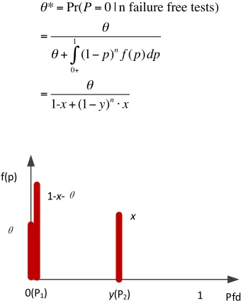
The problem now, as outlined in Section II.A, is to find the most conservative f(p), i.e. the one that minimizes (3) subject to the constraints (1), (2). The value of (3) at the minimum we shall call θ*: this is the most pessimistic posterior belief in perfection consistent with the assessor’s expressed (minimal) prior beliefs.
[image:5.612.391.520.502.582.2]distant7 from the origin with mass 1-x-θ; and at the P
2 point, at
y, with mass x. With this worst case prior f(p), the lower bound of θ, i.e. θ*, is obtained: see equation (4) below. This is the most conservative belief of the assessor about the probability of perfection of this system, after seeing n failure free tests, given his professed prior beliefs (1) and (2).
θ*=Pr(P=0 | n failure free tests)
= θ
θ+ (1−p)nf(p)dp
0+ 1
∫
= θ
1-x+(1−y)n
⋅x
(4)
Pfd 1 y(P2)
0(P1) θ
1-‐x-‐θ
x f(p)
Fig. 2. The most conservative prior distribution.
C. Numerical Examples
Table I shows some numerical examples, where θ is the priori belief about perfection, x and y satisfy the assessor’s prior belief (2), n is the number of failure-free tests that have been observed, θ* is the posterior belief in perfection.
The final column of the table shows the factor by which the posterior beliefs improve on the prior ones. We have chosen to do this in terms of the proportional reduction in the doubt (1-θ) about perfection, since this seems better to reflect intuition here for the values of θ close 1 that we would anticipate in the critical applications that are our concern. So the ratio (1-θ
)/(1-θ*) is the “doubt reduction factor”. Clearly we seek large values of this factor.
In each case there is some increase in the assessor’s confidence in perfection as the number of failure free tests increases. However, this increase in confidence is very modest in all cases: the evidence from failure-free testing seems to be generally very weak in supporting claims about probability of perfection in this worst case.
7Of course our intuitive language is somewhat informal here. To explain more carefully, the worst case posterior belief (3) is, under these constraints, approached as a limit, without being attained exactly by any individual prior
pfd distribution. So to argue with full mathematical rigour entails an infinite
set of distinct prior pfd distributions, each with its own P1>0; with this set so constructed that zero is the infimum of all its member distributions’ positive
P1s. Figure 2 is intended to depict this infimum property of this set of distributions. The infimum of the resulting set of Bayesian posterior perfection probabilities – each computed from one member of this set of priors – is easily show to be the RHS of equation (4).
Notice that the best results in support of perfection in Table I arise when θ and x are larger, i.e. 1-x-θ is small. Now this is the probability mass arbitrarily close to 0 for the most conservative prior distribution satisfying the assessor’s stated prior beliefs. The role this probability mass plays is best understood by seeing what happens when the number of failure-free demands, n, approaches infinity. The conservative bound on probability of perfection is then:
) 1 ( 1
) 1 ( -1 lim
n θ θ
θ θ
θ
− − + = − = ⋅ − + +∞
→ x yn x x x
(5)
[image:6.612.93.268.129.346.2]So even for an infinite number of failure-free demands, the assessor does not become certain of perfection. Informally, when we see an infinite number of failure-free demands, we become certain that pfd cannot be greater than or equal to y; so the only possibilities remaining are perfection and 0<pfd <y. In the case of the second of these, an infinite number of failure-free demands suggests that the probability mass in this interval will be concentrated at the extreme left of the interval. So, the infinite number of demands are failure-free because either (a) the program is perfect, or (b) it is not perfect but has an infinitesimally small failure rate. The probability that what has been seen is due to (a), rather than (b), is just the ratio of Pr(a) to Pr(a or b), i.e. (5) above.
TABLE I.NUMERICAL EXAMPLES OF THE 3 POINTS PRIOR DISTRIBUTION
θ x y n θ*
Doubt reduction
factor: (1-θ)/(1-θ*)
0.5 0.01 0.001 1000 0.503181641 1.006404032 0.5 0.01 0.001 10000 0.505050275 1.010203611 0.5 0.01 0.001 100000 0.505050505 1.010204082 0.5 0.05 0.001 1000 0.516323692 1.033749207 0.5 0.05 0.001 10000 0.526314538 1.055552767 0.5 0.05 0.001 100000 0.526315789 1.055555556 0.9 0.01 0.001 1000 0.905726953 1.060748572 0.9 0.01 0.001 10000 0.909090494 1.099994981 0.9 0.01 0.001 100000 0.909090909 1.10 0.9 0.05 0.001 1000 0.929382645 1.41608249 0.9 0.05 0.001 10000 0.947366169 1.899918692 0.9 0.05 0.001 100000 0.947368421 1.90
Informally, there is a limit to how much confidence in perfection can be obtained from failure-free demands, as we cannot tell whether this happened because of perfection or very high reliability.
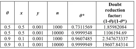
If the assessor were able to rule out very high reliability a priori, of course, this picture changes. Table II shows what happens if 1-x-θ=0, i.e. the expert is certain that the pfd is either 0 or greater than or equal to y. Here, relatively modest numbers of failure-free demands result in high confidence in perfection. These results are intuitively obvious because, for any value of y, the more failure-free working, the more confident we shall be that the system is “perfect” rather than “has a pfd worse than y”.
[image:6.612.325.561.343.502.2]anywhere between 0 and y. Such beliefs do not seem reasonable, of course.
TABLE II NUMERICAL EXAMPLES OF THE CASE 1-x-θ =0OF THE 2 POINTS PRIOR DISTRIBUTION.
θ x y n θ*
Doubt reduction
factor: (1-θ)/(1-θ*)
0.5 0.5 0.001 1000 0.7311569 1.85982084 0.5 0.5 0.001 10000 0.9999548 1106194.69 0.9 0.1 0.001 1000 0.9607485 2.547673337 0.9 0.1 0.001 10000 0.9999949 19607.84314
In the next section we consider what reasonable further restrictions can be placed on an assessor’s prior beliefs, and how these affect his posterior belief in perfection.
III. REFINING THE SET OF ALLOWABLE PRIOR BELIEFS
The results above arise from a situation in which an assessor has expressed some precise, but very limited prior beliefs, represented by (1) and (2). Because these beliefs are so very limited, they are satisfied by a large set of possible prior distributions. In this section we argue that some of these distributions would be ruled out as possible priors by all “reasonable” assessors. The effect of this would be to “prune” the set of allowable priors (still satisfying (1) and (2), of course). An assessor would then proceed as above, but with this pruned – i.e. smaller – set of allowable distributions. That is, he would choose the most conservative of these to find a new posterior probability of perfection.
How should such pruning be carried out? Are there obviously unreasonable distributions in the set of priors that are allowable above?
The conservative results represented by Table I and the limiting result (5) arise essentially because they are based on the most extreme priors that have probability mass at 0+ and y, as well as at 0 (the perfection point). The problem here – what we believe to be the unreasonable “extremeness” of these priors – lies in their having positive support at points in (0,1].
For instance, a frequent situation is that the support for such prior beliefs comes from generic experience of the reliabilities achieved by similar development processes, in products that are comparable to the present one, e.g. in terms of application area, complexity and software engineering culture. Then, while it would seem reasonable for an assessor possibly to believe a non-zero probability of perfection – i.e. mass at 0 for his prior distribution for pfd – it does not seem reasonable for him to believe there is positive mass associated with any non-zero value of pfd. That is, statements like: “I think there is a 50% probability that the pfd is zero, i.e. that this program is perfect” seem reasonable; but statements like “In the event that this program is not perfect, I believe that there is a 20% chance that its pfd is exactly 0.1234” would generally not seem
reasonable8. More precisely, we believe that assessors would usually think that the only beliefs they could reasonably hold would correspond to distributions that satisfy these conditions:
• There is no non-zero probability concentrated at points in (0,1], i.e. the only mass-at-a-point on the complete prior for pfd is that at 0, corresponding to perfection;
• There is no point in (0,1] for which the probability density is zero, i.e. no value is impossible.
These conditions suggest that the only distributions that assessors should normally consider as candidates to represent their prior beliefs should have probability mass only at 0, and have continuous density in (0,1].
Whilst imposing these conditions will eliminate many distributions from the set that simply satisfies (1) and (2), there will still remain a large set of candidate distributions: essentially any suitably renormalized continuous distribution on (0,1], together with a mass at 0.
To then analyse the implication of beliefs like those in (1) and (2), the next stage after this pruning would be to explore the implications of prior distributions in the set thus restricted; possibly eliciting more detailed approximate representations for, or bounds on, the distributions. Which mathematical form these approximations should take will be a matter of convenience, both in elicitation (where the concern is to make it easier for the assessor to translate his reasoning into a distribution without being biased by artificial constraints – e.g. that his beliefs should be represented by a specific parametric family) and calculations (to avoid excessive computational load, avoid excessive numerical errors, and perhaps allow analytical treatment for better insight). We do not address here the question of which representation would be most convenient in a specific case, but develop, purely by way of illustration, an example in which the assessor is prepared to restrict the expression of his prior beliefs to a (suitably renormalized) Beta distribution, on (0,1], with parameters (a,b). We shall discuss later the reasonableness of such a restriction to this Beta parametric family.
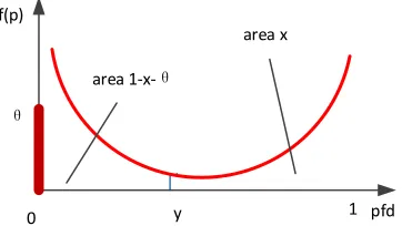
Table III shows the results of numerical optimization to find the most conservative prior within the new restricted set of allowable distributions. Once again, confidence in perfection increases slowly even for very large n. However, it is notable that in all cases in Table III both a and b are fractional, i.e. the most conservative priors in this refined set of allowable distributions are all “U-shaped” as shown in the Fig.3. In each case the probability density is infinite at both 0 and 1.
pfd 1 y
0 θ f(p)
area 1-‐x-‐θ
[image:8.612.371.525.79.197.2]area x
Fig. 3. The most conservative prior re-normalized beta distribution.
We again argue that this kind of U-shaped distribution would not represent the beliefs of reasonable assessors. We can further prune our set of allowable distributions by ruling out such U-shaped beta distributions: if a and b are not allowed to be fractional – i.e. a≥1, b≥1 – we obtain uni-modal beta distributions9.
Optimizing (numerically) over this further-refined set of allowable distributions we obtain the results in Table IV. The worst case conservative results here give large increases in the posterior probability of perfection as n increases; this contrasts with the results we obtained for the less constrained sets of allowable priors, shown in Tables 1 and 3.
The shape of the worst case distributions in Figure 4 are similar to the idealized case of Figure 1: because a is close to 1 and b is large, in each case, they have a mode at (a-1)/(a+b-2), far to the left and very close the origin, but in all cases there is zero probability density at 0 and at 1 (because both a and b are larger than 1).
In fact, the “worst case” results of Table IV are only worst within the accuracy of the numerical optimisation we used. We believe (but have so far not been able to prove!) that the asymptotic optimum – i.e. the true worst case – occurs when
a=1, and to satisfy the percentile constraint, b=log1−yx/ (1−θ). The results for this case are shown in Table V.
Within the “probability mass at 0 plus re-normalised Beta distribution” framework, these results are the most conservative with respect to the assessor’s expressed prior beliefs, and (subject to our “prunings” of the original large class of priors satisfying (1) and (2)) they can be thought of as “no more conservative than they need be.”
We just note here that the numerical values obtained above for the posterior probability of perfection seem potentially useful, but we make no claim for the practical plausibility of the vector of numbers (x, y, θ) we have used for illustration.
Note that in this case, as n goes to infinity, the assessor approaches certainty that the system is perfect.
9By “uni-modal” here we include those cases where the maximum of the density is at the end of the interval, and is not a turning point: this turns out to be the case for a=1 in Table V.
pfd 1 y
0 θ f(p)
area 1-‐x-‐θ area x
Fig. 4. The most conservative prior re-normalized unimodal beta distribution after “pruning”. This is an idealised representation: in reality the “spike” would be very large and close to the origin.
IV. DISCUSSION AND CONCLUSION
The work reported here was, of course, specifically addressing the problem of assessing confidence in perfection of software. However, to do this within the Bayesian framework we have had to consider some difficult general problems concerning prior distributions, so our results may have wider applicability.
We believe that the Bayesian approach is the most appropriate formalism for the assessment of the dependability of critical systems, but its use poses some difficulties for an assessor. The most obvious difficulties concern the need for the assessor to express his prior beliefs about his problem’s unknowns, formally and quantitatively, in order to feed into the formalism of Bayes’ theorem. It is well-known that this can be difficult, and has been used by some to argue that the Bayesian approach is impractical. Assessors are rarely able to provide a complete account of their uncertainty about the unknowns – in terms of the problem addressed in this work, they are unable to express their prior beliefs in a complete distribution for the unknown pfd of the system under study.
[image:8.612.88.269.82.184.2]TABLE III NUMERICAL EXAMPLES FOR THE PRIOR BETA DISTRIBUTIONS WITH MASS AT ORIGIN
θ x y n a b θ* Doubt
reduction factor: (1-θ)/(1-θ*)
Doubt reduction compared with not using the Beta family prior
0.5 0.01 0.001 1000 0.00019256 0.010154142 0.505055848 1.010214987 1.003786705 0.5 0.01 0.001 10000 0.000174069 0.009065462 0.505179928 1.010468306 1.000262021 0.5 0.01 0.001 100000 0.000226364 0.012069137 0.50532834 1.010771468 1.000561655 0.5 0.05 0.001 1000 0.001997401 0.0208142 0.526603047 1.056196068 1.02171403 0.5 0.05 0.001 10000 0.00058413 0.00547856 0.526730227 1.056479895 1.000878334 0.5 0.05 0.001 100000 0.000942005 0.009070504 0.527517591 1.058240457 1.00254359 0.9 0.01 0.001 1000 0.001371121 0.013629679 0.909150688 1.100723798 1.037685864 0.9 0.01 0.001 10000 0.000873768 0.008366982 0.909298034 1.102511938 1.002288154 0.9 0.01 0.001 100000 0.000771203 0.007326781 0.909423631 1.10404073 1.003673391 0.9 0.05 0.001 1000 0.007752825 0.008651361 0.94759435 1.908191213 1.347514165 0.9 0.05 0.001 10000 0.001784232 0.001829209 0.947621395 1.909176459 1.004872717 0.9 0.05 0.001 100000 0.002078817 0.002139551 0.947905689 1.91959541 1.010313374
TABLE IV NUMERICAL EXAMPLES OF THE PRIOR UNIMODAL BETA DISTRIBUTION WITH MASS AT ORIGIN
θ x y n a b θ* Doubt
reduction factor: (1-θ)/(1-θ*)
Doubt reduction compared with not using the Beta family prior
0.5 0.01 0.001 1000 1.002865687 3919.454939 0.556728757 1.127977526 1.120799888 0.5 0.01 0.001 10000 1.000348556 3913.798799 0.780539772 2.278317141 2.255304887 0.5 0.01 0.001 100000 1.000219221 3914.753876 0.963720105 13.78173798 13.6425285 0.5 0.05 0.001 1000 1.001096111 2304.159264 0.589248898 1.217282187 1.177541109 0.5 0.05 0.001 10000 1.000879434 2302.601846 0.842539329 3.175396105 3.008277941 0.5 0.05 0.001 100000 1.001000815 2302.579322 0.978069486 22.79928354 21.59932125 0.9 0.01 0.001 1000 1.000493405 2302.371071 0.928116048 1.39113109 1.311461667 0.9 0.01 0.001 10000 1.000013517 2300.871174 0.97964033 4.911670911 4.465175748 0.9 0.01 0.001 100000 1.001562038 2304.529699 0.997518052 40.29093267 36.62812061 0.9 0.05 0.001 1000 1.002947755 695.838612 0.956506003 2.299167843 1.623611519 0.9 0.05 0.001 10000 1.000263576 693.2090557 0.992853625 13.99310937 7.365109587 0.9 0.05 0.001 100000 1.001273649 694.1325914 0.999239476 131.4883667 69.20440352
TABLE V THE CASE OF THE PRIOR BETA DISTRIBUTION WITH a=1 AND MASS AT ORIGIN.
θ x y n a b θ* Doubt
reduction factor: (1-θ)/(1-θ*)
Doubt reduction compared with not using the Beta family prior
In Section III we discuss ways in which it may sometimes be possible to rule out the second of these explanations. The result in Section II can be seen as a problem that stands in the way of anyone trying to use the results of our earlier work reported in [9, 10]. These results provide a novel means of assessing the pfd of a 1-out-of-2 system in which one channel is sufficiently simple as to be “possibly perfect”. However, they depend upon an assessor being able to make probabilistic claims about perfection, but do not tell an assessor how to do this. That our the main aim in the present paper.
We have described our general approach in three stages (although they need not occur in this order). Firstly we assume that, although he cannot provide a full probabilistic description of his uncertainty, the assessor can express some partial but
precise beliefs about the unknowns. Secondly, we assume that in the inevitable presence of such incompleteness, the Bayesian analysis needs to provide results that are guaranteed to be conservative (because the analyses we have in mind relate to critical systems). Finally, we seek to prune the set of prior distributions that the assessor finds acceptable in order that the conservatism of the results is no greater than it has to be.
On the first point, we assume that the assessor’s prior beliefs about system pfd are expressed in terms of just a prior probability that this pfd is zero (i.e. the system is perfect), together with a single percentile (because, in the event that the system is not perfect, its pfd may lie anywhere in the interval (0,1]): the assessor’s prior beliefs are summarized in the numbers x, y, and θ in (1) and (2).
Of course, these are rather “weak” beliefs. They fall far short of a complete distribution for the unknown pfd. Our next step is to find the most conservative of the many possible complete prior distributions, i.e. the one that gives the most pessimistic value for the posterior probability of perfection. It turns out that this is very conservative – probably too much so to be of practical use.
We therefore proceeded (second stage) to “prune” the infinite set of initially allowable prior distributions, discarding those that we argue all reasonable assessors would find unacceptable, and find the most conservative member of this new set of allowable priors. The corresponding most conservative posterior probability of perfection will be less conservative than the previous one.
There is a sense in which this pruning process makes the assessor’s expressed prior beliefs more extensive than they were: it adds further assessor belief to those previously expressed. But note that, in contrast to the specific and positive
assertions of a (hypothetical) real assessor represented by (1) and (2), this pruning process involves general and negative
assertions about prior distributions: we are identifying proper-ties that no prior distribution, for any reasonable assessor, should possess. We do not need to have a particular assessor in mind to do this.
This is an important point that may be worth labouring a little. We want to emphasise that the pruning process we describe here does not mean that an assessor retrospectively changes his prior beliefs after he has seen evidence that produces embarrassingly inconvenient posterior consequences.
That would be a perversion of a correct assessment process (and, of course, would be considered unacceptable within the Bayesian framework). Rather we (the authors of this paper) believe that some distributions can be discarded because they are unreasonable in general (for a broad class of situations, as discussed earlier), and are thus so in particular for this assessor. In a real dependability case, of course, we would expect that the assessor would expressly agree that the reasons behind this pruning of the set of allowable distributions did in fact accord – or not – with his beliefs.
This general account of our procedure suggests that it may have wider applicability than to the perfection arguments of this paper; we have not seen our approach reported elsewhere.
We now return to the specifics of the reasoning about perfection that was the spur to this work. In particular, are the details of the particular prunings that we have used here supportable?
We have argued earlier why it is reasonable – in a broad class of cases – to rule out finite probability mass arbitrarily close to the origin.
The third stage was to analyse specific representations of the “pruned” set of prior distributions. Here we developed an example using a Beta distribution family for this continuous part of the prior for pfd. This choice can most certainly be questioned. We would claim no more for the choice of a Beta than that it allows us to illustrate our general approach in what follows10.
Since the unrestricted Beta family includes U-shaped distributions with infinite density at 0 and/or 1, we further prune the set of allowable priors to exclude these, i.e. constraining both a and b to be no smaller than 1. The most conservative posterior probabilities of perfection within this set of prior distributions now increase significantly as the number of failure-free demands, n, increases. If the reader – or, more accurately, our (hypothetical) assessor – has accepted our reasoning thus far, these results allow appropriate testing evidence to provide useful confidence in perfection of a system.
Given our interest in probability of perfection, readers may reasonably ask whether the results we have obtained here are special to the Beta distribution assumption, or are more widely applicable. In particular, can we expect to gain increasing confidence in perfection of software by observing large numbers of failure-free demands, under different assumptions? We have no definitive answer to this question. But we speculate tentatively that the conditions we imposed to prune the Beta family here are rather weak, and similar restrictions
may be available for a wide class of assumed distribution families.
Using any particular parametric family of priors, as in our example using the Beta here, may be regarded as a “strong” assertion for an assessor. For example, in some safety-critical industries, a regulator with responsibility for oversight might reasonably respond: “You may represent your prior beliefs by this Beta family, but this seems unreasonably restrictive to me, so I cannot accept as reasonable the resulting claims you make for the probability of perfection.” Is it possible to impose weaker constraints on the form of the prior distribution – i.e. more “generally believable” ones – than the choice of a parametric family of distributions? One might, for example, try to state optimization constraints on only the general form of prior distribution, such as perhaps just its unimodality on (0,1]. Our Tables 4 and 5 show some results attained by unimodal priors which are constrained to be beta: what would we find were we able to remove the Beta family constraint but retained that of unimodality? We do not currently know. One can easily imagine other general classes of simple constraint for which similar questions can be asked: an upper or lower density bound, perhaps, or constraints involving distribution moments. These questions suggest possible avenues for further investigation into constrained worst cases priors which might help us to understand better the implications of what we have observed for our Beta example.
Finally, we note that failure-free working is not the only evidence that can be used to support claims about the reliability, or perfection, of software. Other software engineering measures and metrics have been proposed in the past to aid quantitative prediction of software reliability: see, e.g. [18, 19]. Whilst such evidence is generally not sufficient on its own to obtain accurate predictions of reliability [20], we speculate that it may help assessors to provide the partial prior beliefs we need in our conservative inference, and perhaps to justify specific prunings. In particular, evidence from formal verification seems, on intuitive grounds, to be especially attractive [14] as a means to support claims about perfection. Whilst this kind of evidence does not currently fit readily into the kind of Bayesian analysis we are using here, we think an assessor might use it informally to support his (limited) subjective prior beliefs. More formal support for this kind of reasoning is clearly needed These are some of the issues we intend to address in further work.
ACKNOWLEDGEMENTS
The work reported here was supported by the UK C&I Nuclear Industry Forum (CINIF). We are grateful for comments on the paper from CINIF representatives Andrew White and Silke Kuball. The views expressed in this paper are those of the author(s) and do not necessarily represent the views of the members of the C&I Nuclear Industry Forum (CINIF). CINIF does not accept liability for any damage or loss incurred as a result of the information contained in this paper.
REFERENCES
[1] Federal Aviation Administration Advisory Circular (1985), AC 25.1309-1A.
[2] HSE (2013). GDA Step 4 and Close-out for Control and Instrumentation Assessment of the EDF and AREVA UK EPR Reactor. Bootle, Health and Safety Executive, Office for Nuclear Regulstion.
[3] Littlewood, B. and Strigini, L. (1993). “Validation of ultra-high dependability for software-based systems.” CACM 36(11): 69-80. [4] Littlewood, B., Popov, P. and L. Strigini. (2002). “Modelling software
design diversity - a review.” ACM Computing Surveys 33(2): 177-208. [5] Boeing (2013). “Statistical Summary of Commercial Airplane
Accidents, Worldwide Operations, 1959-2013.” Seattle, Aviation Safety, Boeing Commercial Airplanes.
[6] Knight, J. C. and Leveson, N. G. (1986). “An experimental evaluation of the assumption of independence in multi-version programming,” IEEE Transactions on Software Engineering, vol. SE-12, no. 1, pp. 96-109, Jan.
[7] Eckhardt, D.E., Caglayan, A.K., Knight, J.C., Lee, Larry D., McAllister, D.F., Vouk, M.A., Kelly, J.P.J.. (1991). “An experimental evaluation of software redundancy as a strategy for improving reliability.” IEEE Trans Software Eng. 17(7): 692-702.
[8] Littlewood, B. and Miller, D. R. (1989). “Conceptual modelling of coincident failures in multi-version software,” IEEE Transactions on Software Engineering, vol. 15, no. 12, pp. 1596-1614, Dec.
[9] Littlewood, B. and Rushby, J. (2012). “Reasoning about the Reliability of Diverse Two-Channel Systems in which One Channel is ‘Possibly Perfect’”, IEEE Transactions on Software Engineering, vol. 38, no. 5, pp. 1178-1194.
[10] Littlewood, B. and Povyakalo, A. A. (2012). “Conservative Reasoning about the Probability of Failure on Demand of a 1-out-of-2 Software-Based System in Which One Channel Is ‘Possibly Perfect’”, IEEE Transactions on Software Engineering, vol. 39, no. 11, pp. 1521-1530. [11] Littlewood, B. and Wright, D. (1997) “Some Conservative Stopping
Rules for the Operational Testing of Safety-Critical Software.” IEEE Transactions on Software Engineering, vol. 23, no. 11, pp. 673-683. [12] Strigini, L. and Povyakalo, A. A. (2013). “Software fault-freeness and
reliability predictions” Paper presented at the SAFECOMP 2013, 32nd International Conference on Computer Safety, Reliability and Security, 24 - 27 September 2013, Toulouse, France.
[13] Bishop, P., R. Bloomfield, Littlewood, B., Povyakalo, A., Wright, D.. (2011) “Towards formalism for conservative claims about the dependability of software-based systems.” IEEE Transactions on Software Engineering 35(5): 708-717.
[14] Littlewood, B. and Wright, D. (2007) “The Use of Multi-Legged Arguments to Increase Confidence in Safety Claims for Software-Based Systems: A Study Based on a BBN of an Idealized Example” IEEE Transactions on Software Engineering vol. 33, no. 5, pp. 347-365. [15] Rushby, J. (2009) “Software Verification and System Assurance,” Proc.
Seventh Int’l Conf. Software Eng. and Formal Methods, D.V. Hung and P. Krishnan, eds., pp. 3-10, Nov. 2009.
[16] Health and Safety Executive (1992), “The tolerability of risk from nuclear power stations”, HMSO, London.
[17] Bertolino, A. & Strigini, L. (1998). “Assessing the Risk due to Software Faults: Estimates of Failure Rate versus Evidence of Perfection,” Software Testing, Verification and Reliability, 8(3), pp. 155-166. [18] Li, M. and Smidts, C. (2000), “A Ranking of Software Engineering
Measures Based on Expert Opinion,” IEEE Transactions on Software Engineering, Vol 29, No 9, pp 811-824, Sept 2003.
[19] Smidts, C. and Li, M. (2000), “Software Engineering Measures for Predicting Software Reliability in Safety Critical Digital Systems,” NUREG/GR-0019, Nuclear Regulatory Commission, Washington DC, November 2000.
APPENDIX
The problem is to find the most conservative prior distribution f(p), still satisfying (1) and (2), which minimizes (3), then calculate the corresponding posterior probability mass at the origin, θ*.
By the mean value theorem for integrals, we could find two values, say P1 and P2, satisfying the equations below,
∫
∫
+ + − = y n y dp p f p dp p f 0 0 n1 ( ) (1 ) ( )
P
-1 )
( (6)
∫
∫
= − 1 1 y n2 ( ) (1 ) ( )
P -1
y
nf pdp
p dp p f )
( (7)
where 0<P1<y, y≤P2≤1. From the prior constraints (1) and (2), we know:
f(p)dp=
0+
y
∫
1−x−θ∫
=1
y ) (pdp x f
So we get,
∫
+ − = − − ynf pdp
p x
-P
0 n
1) (1 ) (1 ) ( )
1
( θ (8)
∫
−= ⋅
1 n
2 (1 ) ( ) 1
y
nf pdp
p x
-P)
( (9)
Put (8) and (9) into (3), we get,
x -P x -P dp p f
pn + − − + ⋅
= − + =
∫
+ n 2 n 1 1 0 1 ) 1 ( ) 1 ( ) ( ) 1 ( * ) ( θ θ θ θ θ θ (10)To minimise (10), we can easily see that when both P1 and
P2 reach their lower bound, θ* reaches its lower bound. That is, when P1=0 and P2=y,
x y) ( x θ x P θ) x ( ) -P ( θ θ
θ* n n n
− + − ≥ ⋅ − + − − + = 1 1 ) 1 ( 1
1 1 2