A group contribution method for predicting the solubility of mercury

A group contribution method for predicting the solubility of mercury

Mansour Khalifaa,∗_{, Leo Lue}a

a_{Department of Chemical and Process Engineering, University of Strathclyde, James Weir Building, 75 Montrose Street, Glasgow G1 1XJ,}

United Kingdom

Abstract

Mercury is a toxic and corrosive element, and understanding its partitioning within ecosystems and industrial pro-cesses is of vital importance. The solubility of mercury in normal alkanes, aromatics, water and alcohols is predicted using widely used Soave-Redlich-Kwong equation of state in combination with a group contribution method to esti-mate binary interaction parameters. The interaction parameters between elemental mercury and seven other molecular groups were determined in this work by fitting available solubility data for mercury. The solubility in the studied sol-vents was accurately described. This work allows the prediction of the thermodynamic behavior of elemental mercury in a wide variety of solvents, solvent mixtures, and operating conditions where experimental data are unavailable.

Keywords: mercury, solubility, equation of state, group contribution method

1. Introduction

Mercury occurs naturally in the environment and can be found in soil, air, and water. Due to its toxicity and accumulative nature, it is considered a highly dangerous element [1, 2, 3]. The sources of mercury in the bio-sphere can be divided into natural and anthropogenic sources. Both are considered to be equally important causes of mercury accumulation in the environment. Natural sources include volcanic activity, erosion of ter-rain, and dissolution of mercury minerals in the oceans, lakes and rivers [4]. Anthropogenic sources include ce-ment manufacturing, paper milling, the combustion of coal, oil, and gas as fuel to generate power, flared gas from onshore and offshore oil and gas platforms, and produced water discharged from oil and gas processing facilities, refineries and chemical plants [5, 6, 7].

In addition to its contribution to environmental pollu-tion, mercury has a negative impact on the production and processing of oil and gas. As mercury is present in many major oil fields, maintenance and operation teams can be exposed to this highly dangerous element on a daily basis. Activities that expose workers to mercury include equipment cleaning, oil sampling, vessel and tank inspections and hot work activities on restricted areas. The risks are proportional to the concentration

∗

Corresponding author

Email addresses:[email protected]

(Mansour Khalifa),[email protected](Leo Lue)

of mercury in the process facilities [8]. Mercury not only poses health risks, it is also corrosive and can cause equipment degradation and damage, catalyst poi-soning, etc. [9]. It has an ability to accumulate on pri-mary and secondary process treatment units (e.g., amine units, glycol units, cryogenic units and heat exchang-ers), eventually causing process failure [8].

interactions with other compounds, such as process flu-ids (e.g., water, hydrocarbon mixtures, etc.).

Many physical properties of mercury, such as density, thermal expansion and compressibility as a function of temperature and pressure have been measured [11]. Va-por pressure is one of the most imVa-portant properties, as it indicates the state of mercury and its concentration in vapor, liquid, and solid phases. Several experimen-tal measurements and correlations have been published for the calculation of mercury vapor pressure over wide range of temperatures [12, 13].

Predicting the solubility of mercury in liquids and gases gives an indication of mercury pathways from one phase to another. Accurate prediction of mercury solu-bility plays an important role in developing a risk mit-igation strategy. In general, however, the available ex-perimental data are limited, in part, due to the difficulty in working with mercury. Experiments involving mer-cury can be time consuming and costly, and it is difficult to anticipate the wide range of process conditions and fluids that may be encountered.

In situations where experimental data are unavailable, predictive methods are required. A competitive model should be computationally inexpensive to evaluate and require minimal parameterization [14]. One powerful method is molecular simulation, which requires force fields to be parameterized between all species in the so-lution. This work has been focused particularly on sys-tems containing elemental mercury [15] and some mer-cury compounds [16, 15] in water. While these methods offer the possibility of predicting thermodynamic prop-erties of system containing mercury, they are compu-tationally intensive and not suitable for use in process scale simulations (e.g., in a refinery).

Another approach is to use thermodynamic models, such as an equations of state (EOS) or an activity coeffi -cient model [17]. These models have been successfully used for the estimation of physical and chemical prop-erties of pure and multicomponent systems. The selec-tion of a model depends on its capability of estimating the required physical and chemical properties, and pre-dicting the phase behavior of a specific system where experimental data are unavailable. Equations of state, such as cubic equations of state or the perturbed-chain statistical associating fluid theory (PCSAFT), are char-acterized by their simplicity, reliability and robustness over a wide range of conditions (e.g., high pressures), and speed of computation [18]. Therefore, they are the model of choice for many multicomponent systems and are widely used for practical applications.

A recent study used PCSAFT to describe the phase behavior of elemental mercury in liquid and compressed

hydrocarbon gases [19]. While this approach works well, it requires fitting binary interaction parameterski j between mercury and the specific solvents being mod-eled to existing experimental measurements. Properly accounting for the interactions between molecules is vital to the accurate prediction of mixture properties. Within the context of equations of state, this is typi-cally achieved by introducing the binary interaction pa-rameter ki j between different molecular species; ki j is normally used as a fitting parameter that is adjusted to minimize the differences between the calculated and ex-perimentally measured system properties, such as VLE, LLE, density, and solubility. This limits its usage to sol-vents where measurements with mercury exist.

One approach developed in order to overcome this issue is the group contribution method (GCM). In the GCM, molecules are subdivided into a series of groups which consist of individual atoms or collections of atoms [20]. The binary interaction parameters between two molecules is then given as the sum of the interaction parameters between the various pairs of groups on each of the molecules. This allows the prediction ofki j for a large number of compounds where experimental data are unavailable and at operating conditions outside the range of measurements.

In this work, we parameterize a group contribution method to estimate the binary mixing parameters for the Soave-Redlich-Kwong (SRK) equation of state to the estimation of the thermodynamic properties of el-emental mercury in mixtures of water, alkanes, aro-matics, and alcohols. The SRK EOS is used in this work because of its simplicity, computational efficiency, and ability to predict vapor-liquid equilibria (VLE) and liquid-liquid equilibria (LLE) at high and low pressures. The ki j of elemental mercury was predicted using the GCM developed by Peneloux and co-workers [20]. This has the advantage that the group interaction parameters already exist [21, 22, 23] for the SRK EOS for a wide range of molecular groups, and so the method can be immediately used in practical calculations. Combined with a group contribution method, the SRK EOS allows the prediction of mercury solubility and partitioning be-tween phases.

2. Methodology

The SRK EOS is a modification of a cubic equation of state proposed by Redlich and Kwong [24] developed by Soave [25] by studying the behavior of pure com-pounds:

p= ρRT

1−ρb−

aρ2

(1+ρb) (1)

wherepis the system pressure,T is the absolute tem-perature, and Ris the universal gas constant, ρis the molar density of the system, anda andb are parame-ters of the model. The first term of Eq. (1) corresponds to the repulsive force and the second term corresponds to the attraction force. The parametersai andbifor a pure componentican be expressed in terms of its criti-cal temperatureTciand critical pressurepci

ai=0.42747

R2_T2

ci

pci

αi(T) (2)

αi(T)=

    

1+(0.480+1.57ωi−0.176ω

2 i)     

1−

r T Tci             2 (3)

bi=0.08664

RT2

ci

pci

(4)

whereωiis the acentric factor for component i, intro-duced by Pitzer [17].

To extend the SRK EOS to multi-component systems, mixing rules are required to obtain the parametersaand

bfor the solution from theai’s andbi’s from the indi-vidual pure components. Many mixing rules have been proposed for cubic EOS [26, 27]. In this work, we use the van der Waals mixing rules, which are given by

a=X

i j

xixj √

aiaj(1−ki j) (5)

b=X

i

xibi (6)

whereki jin Eq. (5) is the binary interaction parameter,

xi is the mole fraction of componenti in the mixture, andaiandbiare calculated from Eqs. (2) and (4).

2.1. The Helmholtz Energy

From knowledge of the Helmholtz energy as a func-tion of the temperature, volume, and component densi-ties, all thermodynamic properties of a system can be determined. For an ideal gas, the molar Helmholtz en-ergyAig_{is given by}

Aig(T, ρ)=X i=1

xiµ◦i +RT

X

i=1

xi(lnρibi−1) (7)

whereρiis the molar density of componenti, andµ◦i is the standard state chemical potential.

In order to consider real systems, we define a resid-ual property as the difference between the property of the actual system and that of an ideal gas at the same total volume, temperature and number of moles of each species [18]

Mres(T,V,n)=M(T,V,n)−Mig(T,V,n) (8)

whereMres_{is any residual property.}

The molar residual Helmholtz energyAres_{can be} di-rectly determined from the equation of state by

Ares=RT

Z ρ

0 dρ

ρ (Z−1)=I (9)

whereZ =p/(ρRT) is the compressibility factor, andρ is the molar density of the system.

The compressibility factor for the SRK equation of state can be written as:

Z = 1

1−ρb −

a b2_RT

ρb

1+ρb

=Zexc+Zatt (10)

whereZexc accounts for excluded volume interactions, andZattaccounts for attractive interactions. Substituting Eq. (10) into Eq. (9),Arescan be written as:

Ares=Iexc(ρb)−E(T,x)Q(ρb) (11)

whereIexcis the contribution from excluded volume in-teractions,Echaracterizes the dependence of the attrac-tive interactions in the system on the composition and temperature, and Q captures the influence of density (which is related to the “frequency” of the interactions). For the SRK EOS, these terms are explicitly given by

Iexc(ρb)=−RTln(1−ρb), (12)

E(T,x)= a

b2, (13)

Q(ρb)=ln(1+ρb). (14)

In order to characterize the influence of mixing on a system, we first define an ideal solution, where the Helmholtz energy is defined as:

Aid=X

i=1

xiA◦i +RT

X

i=1

xilnxi (15)

whereA◦

i is the molar Helmholtz energy of pure com-ponenti, which is given by

whereI_i◦is the molar residual Helmholtz free energy of pureiat packing fractionρbi and temperature T. We also define an excess property as the difference between the actual value of the property of the system and the value of an ideal mixture at the same temperature, total moles of each species and packing fraction [18]:

ME(T,n, ρb)=M(T,n, ρb)−Mid(T,n, ρb) (17)

whereME is the excess property and Mid is the ideal mixture property.

The excess Helmholtz free energy at constant temper-ature, constant volume, and constant number of moles of each species can be defined based on Eq. (17) as:

AE(T,n, ρb)=A(T,n, ρb)−Aid(T,n, ρb)

=RTX

i

xiln

bi

b +I−

X

i

xiIi◦.

The first term represents effect of molecule size on the free energy of mixing, while the final two terms give the influence of the attractive interactions between molecules.

For an equation of state similar in form to the SRK EOS, the excess Helmholtz free energy can be written as

AE(T,n, ρb)=RTX

i

xiln

bi

b + Q(ρb)

2b

X

i,j

xixjbibjEi j

(18)

whereEi j physically captures the free energy of inter-action between a molecule of typeiand a molecule of type j, and theQ term describes the frequency of the interactions. The parameterEi j can be directly related to the original parameters of the SRK equation of state as

Ei j =−2

ai j

bibj

+ ai

b2

i

+aj

b2

j

. (19)

Using the van der Waals mixing rules (see Eqs. (5) and (6)) leads to:

Ei j=(δi−δj)2+2δiδjki j (20)

whereδi=a1_i/2/biis the Scatchard-Hildebrand solubil-ity parameter [17, 22, 28]. So we see that the binary interaction parameterki j describes the deviation of the interaction free energy between two molecules from that given by the regular solution model:

ki j=

Ei j−(δi−δj)2

2δiδj

. (21)

The regular solution model applies to mixtures where molecules are of similar size and interact only through dispersion forces [17]. For mixtures of molecules of different size or where other forces are present (e.g., hy-drogen bonding, dipole-dipole interactions, etc.), devia-tions from this model are to be expected. In this work, this is captured by the mixing parameterki j.

2.2. Group contribution method

In order to obtain accurate results with a cubic EOS, appropriate values for binary interaction parameters are required. Typically, the ki j’s are used as fit parame-ters used to reproduce experimental data. However, fre-quently the experimental data required to develop and validate the thermodynamic models are lacking. Sev-eral empirical methods have been proposed to estimate binary interaction parameters; however, many of these correlations fail to properly predict the phase behavior at elevated pressures [29].

Alternate mixing rules to the van der Waals mixing rule (see Eqs. (5) and (6)) have been proposed as in order to improve the accuracy of EOS’s. One class of these is based on combining the EOS with an activ-ity coefficient model [21] and is typically referred to as EOS/gE_.

The use of group contribution techniques with activ-ity coefficient models, such as UNIFAC, has been quite successful [14]. Calculating an EOS’s parameters based on a group contribution method (GCM) is often more powerful than the use of activity coefficient models and can provide accurate predictions [18, 21]. The combina-tion of an EOS with a group contribucombina-tion method results in a predictive model that provides a theoretical expres-sion forki j

The interaction free energy energy Ei j between a molecule of typeiand a molecule of type j, which ap-pears in Eq. (20), can be expressed in terms of a sum of the interactions between pairs of groups within the molecules [20]

Ei j=− 1 2

X

k,l

(αik−αjk)(αil−αjl)Akl(T) (22)

where the indices kandlrun over all types of groups in the system, andαikis the fraction of moleculei oc-cupied by groupk. For example, propane has a molec-ular structure of CH3-CH2-CH3; It contains two CH3

groups and one CH2group. Therefore the total number

The temperature dependence of the interaction pa-rameterAkl(T) is given by:

Akl(T)=A0_kl

_T0

T

B0kl/A0kl−1

(23)

whereT is the absolute temperature,T0 = 298.15 K is a reference temperature, andA0_klandB0_klare the interac-tion parameters between groupskandl.

The quantity Akl(T) represents the negative free en-ergy of interaction between a group of type k and a group of type l. From the Gibbs-Helmholtz equation [17], we can then identify the quantity

B0_kl

_T0

T

B0kl/A0kl−1

with the attractive energy of interaction between groups, and, consequently, the quantity

A0_kl(B0_kl/A0_kl−1)

_T0

T

B0kl/A0kl−1

is related with the entropy of the interaction.

This group contribution method (GCM) was used by Jaubert and No¨el [21] to predict the VLE of several binary mixture of hydrocarbon components using the Peng-Robinson EOS (PR), calling this the predictive Peng-Robinson 1978 (PPR78). No¨el showed that the obtained results from GCM are often more precise than EOS/gE _{models. Another study used the GCM to} pre-dictki jof a system containing hydrocarbon components and carbon dioxide CO2 using SRK EOS [23]. The

study indicated its feasibility to estimate theki j of any mixture containing carbon dioxide and hydrocarbons at any temperature. A relation between theki jparameters for PPR78 and the SRK EOS has been developed [22]. This helps to predict GCM parameters of SRK EOS based on PR EOS GCM parameters. Consequently, the values for the group interaction parametersA0

klandB

0

kl between a large number of different types of groups is already available.

3. Results and discussion

In this section, we determine the values of the group interaction parametersA0_kl andB0_kl appearing in Eq. (23) between elemental mercury and various molec-ular groups. As an initial step in this process, we need to ensure that the properties of the pure components are properly described by the SRK equation of state. This is done by ensuring the vapor pressure curves are accu-rately reproduced, which is described in the next sec-tion.

Once the pure component parameters of the SRK EOS are chosen, the values of the group interaction pa-rameters are determined by fitting experimental solubil-ity data for mercury in a variety of solvents. This is done by minimizing the objective functionFobj

Fobj=X

i

     

S_icalc−Sexp_i

Sexp_i

     

2

(24)

whereSexp_i is the experimental solubility of mercury in the selected solvent, andScalc_i is the calculated solubility of mercury in the selected solvent.

Vapor-liquid equilibrium (VLE) and liquid-liquid equilibrium (LLE) calculations were performed for the SRK equation of state using standard flash algorithms implemented in Python to obtain the solubility of mer-curyScalc_i . The LmFit package in Python was used to determine the values of the group interaction parame-tersA0

klandB

0

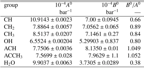
klin Eq. (23) that minimize the objective function. The optimized values and their uncertainties are summarized in Table 1. These are discussed in more detail in the following parts of this section.

Table 1: Group interaction parametersA0 _andB0_{for mercury with}

other groups.

group 10−4_A0 ₁₀−4_B0 _B0_/A0

bar−1 _bar−1 _—

CH 10.9143±0.0023 7.00±0.0945 0.66 CH2 7.8864±0.0057 7.0562±0.065 0.89

CH3 8.5137±0.0207 7.1461±0.27 0.84

OH 6.5524±0.00204 5.29903±0.837 0.80 ACH 7.7506±0.0036 8.1350±0.01 1.049 ACCH3 7.5699±0.028 7.9629±1.1 1.052

H2O 9.9037±0.0063 3.7305±0.0289 0.38

3.1. Vapor pressure

In order to predict the pure component properties of a species, the SRK equation of state requires its criti-cal pressure, criticriti-cal temperature and acentric factor. In principle, these can be obtained

Figure 1 indicates that the SRK EOS is capable of accurately predicting the vapor pressure of elemental mercury, water, and alcohols. The AARD for 99 exper-imental data points of elemental mercury over a tem-perature range of 253.15 K to 773.15 K was 3.7%, the experimental data used in this work were taken from Refs. 30, 31, 32, 33. These data were classified by Hu-ber et al. as primary experimental data, because of their low experimental uncertainty of around 1% [12].

The AARD for the vapor pressure of water was 2.5% for 38 experimental data points over a temperature range of 319.6 K to 449.7 K; the experimental data used in this work were taken from Ref. 34. For methanol and iso-propanol, the AARD was 2.8% for 24 data points and 2.6% for 14 experimental data points, respectively; the experimental data were taken from Ref. 35, 36, 37.

Figure 1: Relative deviation in vapor pressure for elemental mercury (black), water (red), methanol, (yellow), and isopropanol (blue).

Figure 2 shows the relative deviation of the predic-tions of the SRK equation of state for the vapor pres-sure of somen-alkanes and aromatic compounds. The AARD for propane,n-pentane, andn-decane was 0.4% for 31 experimental data points, 0.2% for 50 experimen-tal data points, and 2.5% for 32 experimenexperimen-tal data points respectively. the experimental vapor pressure data were taken from Refs. 38, 39, and 40. In addition, the AARD for the vapor pressure of benzene, toluene, ando-xylene was 0.9% for 13 experimental data points, 0.3% for 17 data points, and 0.78% for 12 data points, respectively; the experimental vapor pressure data for aromatics were taken from Refs. 41,42, and 43.

3.2. Solubility of mercury in water

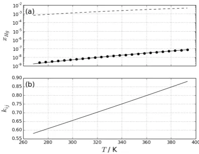
The solubility of elemental mercury in water is avail-able over a wide range of temperatures. The experi-mental data used in this work were taken from Ref. 47,

Figure 2: Relative deviation in vapor pressure of (a)n-alkanes and (b) aromatic compounds.

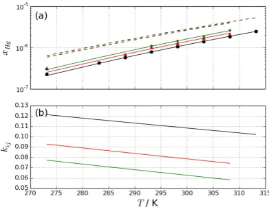
which are shown as the symbols in Fig. 3(a) over a tem-perature range of 273.15 K to 393.15 K. The dashed line in Fig. 3(a) is the solubility of mercury predicted by the SRK EOS, neglecting the binary interaction param-eter (i.e.ki j=0); without introducing proper binary in-teraction parameters, the mercury solubility in water is severely overestimated. The solid line in Fig. 3(a) gives the prediction of the SRK EOS with the ki j shown in Fig. 3(b). For this system, an AARD of 4.2% was ob-tained for 25 experimental data points. The binary in-teraction parameter between mercury and water is tem-perature dependent; it increases by 0.05 with each 20 K increase in temperature.

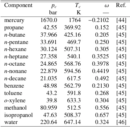
Table 2: Pure component critical properties and acentric factor.

Component pc Tc ω Ref.

bar K —

mercury 1670.0 1764 −0.2102 [44]

propane 42.55 369.92 0.152 [45]

n-butane 37.966 425.16 0.205 [45]

n-pentane 33.691 469.7 0.250 [45]

n-hexane 30.124 507.31 0.305 [45]

n-heptane 27.358 540.1 0.3525 [45]

n-octane 24.865 568.76 0.3978 [45]

n-nonane 22.879 594.56 0.4419 [45]

n-decane 21.035 617.5 0.492 [45] benzene 48.98 562.79 0.2130 [45]

toluene 43.2 591.8 0.268 [45]

o-xylene 39.8 633.3 0.304 [45]

methanol 80.959 512.5 0.556 [45] isopropanol 47.63 508.37 0.657 [45]

water 220.64 647.14 0.324 [46]

Thermodynamically, the ratioB0/A0 reflects the in-fluence of entropy on the mixing of groups. If the ratio is less than one, the mixing process tends to increase entropy; the molecules become more disordered than in ideal mixing. If the ratio is greater than one, then en-tropy is lost in mixing; the molecules are more ordered than in ideal mixing. For a ratio of one, there is no excess entropy of mixing and, and enthalpy drives the process. In this case, the binary interaction parameter temperature independent.

3.3. Solubility of mercury in normal alkanes

Normal alkanes represent more than 90% of natural gas and crude oil species. Predicting mercury solubility in these species is crucial. Elemental mercury is con-sidered the dominant mercury species in the crude oil and natural gas [9, 48]. The solubility data of elemental mercury in hydrocarbon systems are sparse and covers a limited temperature range, The experimental data used in this work are shown as the symbols in Fig. 4(a) and (b) for alkanes from C5 to C10, and Fig. 5(a) and (b)

for C3 and C4. These data were taken from Ref. 49

and Refs. 50 . Around 65 experimental data points for C5 to C10 over a temperature range of 273.15 K to

336.15 K and atmospheric pressure, and 3 experimen-tal data points for C8 over a temperature range from

338.15 K to 473.15 K and 6 bar. In addition to 17 data points for C3and C4at different temperatures and

pres-sures.

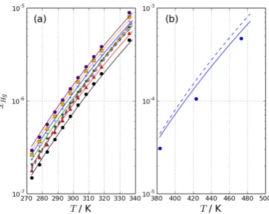
Figures 4(a) and (b) show the predicted solubility of elemental mercury in normal alkanes from C5 to C10.

The dashed lines in Fig. 4 are the solubilities predicted by the SRK EOS, neglecting the binary interaction pa-rameter (i.e. ki j = 0); without introducing the proper binary interaction parameters, the mercury solubility in alkanes is nearly independent of the molecular weight of the alkanes. By introducing the binary interaction pa-rameter, the results indicated by the solid lines in Fig. 4 are obtained. The AARD for the solubility in normal alkanes from C3to C10 was 5.47% for 74 experimental

data points.

In the recent study of Polishuk et al. [19], the Peng-Robinson (PR) and PC-SAFT equations of state were used to predict the properties of mercury-hydrocarbon mixtures. In their work, a single, constant value of

ki j, which was fixed by fitting to experimental solubility data of mercury inn-pentane, was used. The results of the study showed that within this approach, the Peng-Robinson EOS was incapable of estimating the solu-bility of mercury in the studied hydrocarbon systems, apart from mercury-pentane. The results presented in Fig. 3 of Polishuk et al. show that the predicted sol-ubility of mercury in C8 using PC-SAFT and the PR

EoS at 298.15◦C was 0.91 ppm and 3.5 ppm, respec-tively, while the experimental solubility was 1.08 ppm. The value obtained in this study using the GCM was 1.10 ppm which is much closer to the experimental value.

In our study, differentki j values were calculated us-ing GCM for each mercury-hydrocarbon binary system at the system temperature and pressure. This approach improves the prediction of mercury solubility in normal alkanes more accurately than fixingki jto a single value. The solubility of elemental mercury increases with the carbon numbers, which is in consistent with the obser-vations of Refs. 49 and 50.

Several process facilities, such as stripping columns, heat exchangers, reactors, and distillation units operate at high temperatures; therefore, predicting mercury ubility in alkanes at high temperature is crucial. The sol-ubility of elemental mercury in some organic solvents, including octane, dodecane, and toluene, has been ex-perimentally and theoretically estimated over a temper-ature range from 100◦C to 200◦C and up to 6 bar [50]. Figure 4(b) represents the predicted solubility of ele-mental mercury in normal octane at 6 bar and high tem-peratures.

hy-Figure 4: Solubility of mercury in normal alkanes: C5(black), C6

(red), C7(green), C8(blue), C9(orange), and C10(indigo). The

sym-bols represent experimental data, the solid lines represent predicted solubility with the binary interaction parameters estimated using the GCM, and the dashed lines represent the solubility without introduc-ing the binary interaction parameter.

drocarbons well. This is due to fact that cubic EOS’s are capable of predicting vapor phase properties more accu-rately than liquid phase properties. It can be noticed that the solubility of elemental mercury in propane is almost equal to that in butane. This implies that the solubility of mercury in light hydrocarbons in the gas phase is dependent of carbon number. This suggests that the in-teraction of elemental mercury with methane or ethane is similar to that with propane and butane. This enables the estimation of mercury solubility in methane, as the experimental data are unavailable.

The binary interaction parameters of mercury in nor-mal alkanes from C5to C10are shown in Fig. 6. The

in-teraction of mercury with these higher molecular weight alkanes depends on both the carbon number and temper-ature.

3.4. Solubility of mercury in aromatics

Aromatics are considered to be the main raw material for many petrochemical industries [51]. The naphtha reforming process is one of main sources of aromatics. As crude oil and natural gas are the main sources of aromatics and crude oil is known to contain mercury, predicting the solubility of mercury in aromatics is vital of importance.

Figure 7(a) shows the solubility of elemental mer-cury in benzene, toluene, and o-xylene over a range of temperatures. The experimental data are taken from Ref. 49, which are shown as the symbols. The dashed lines are the predictions of the SRK EOS withki j =0.

Figure 5: Solubility of mercury in (a) propane and (b) butane.

Figure 6: Binary interaction parameter for mercury-alkane mixtures.

It is clear that by neglecting the binary interaction pa-rameters, the predicted solubility of elemental mercury in aromatics is relatively insensitive to the presence of methyl groups.

Figure 7: (a) Solubility and (b) binary interaction parameter of mer-cury with in benzene (black), toluene (red), ando-xylene (green).

The solid lines in Fig. 7(a) show the solubilities cal-culated by the SRK EOS with the binary interaction pa-rameters estimated by the group contribution method. As a test of the group contribution model, the binary in-teraction parameter between mercury and toluene was predicted based on the group interaction parameters obtained from mercury-benzene and mercury-o-xylene mixtures. The AARD for mercury in benzene, toluene, ando-xylene was 1.87% for 8 data points over a tem-perature range of 273.15 K to 313.15 K, 6.1% for 6 data points over a temperature range of 273.15 K to 308.15 K, and 2.7% for 5 data points over a temperature range of 273.15 K to 308.15 K and atmospheric pres-sure, respectively.

The results presented in Fig. 4 of the Polishuk et al. [19] study show that the predicted solubility of mercury in toluene using PC-SAFT and PR EoS at 293.15◦_{C was} 0.91 ppm and 1.05 ppm, respectively, while the experi-mental solubility was 0.98 ppm. The value obtained in this work using the GCM and based on the group inter-action parameters obtained from mercury-benzene and mercury-o-xylene mixtures was 0.94 ppm, which better reflects the experimental value. The GCM is capable of predicting binary interaction parameters of compounds where experimental data are unavailable.

By introducing binary interaction parameters, the sol-ubility of elemental mercury in aromatics is found to increase with the number of methyl groups, which is consistent with what is experimentally observed. Fig-ure 7(b) indicates that the interaction between mercury and aromatics is fairly independent of temperature.

3.5. Solubility of mercury in alcohols

Alcohols such as mono-ethylene glycol (MEG) and diethylene glycol (DEG) are widely used in oil and gas processing as anti-freeze and anti-corrosion agents; however, experimental data for the solubility of mercury in these alcohols are not available in the literature. One of the motivations of this work is to predict mercury sol-ubility in such alcohols.

Experimental data are available for the solubility of mercury in methanol and isopropanol [47]. Figure 8(a) shows a comparison of the SRK EOS, with and without the binary interaction parameter, and experimental mea-surements for the solubility of mercury in methanol and isopropanol. Significant deviation can be observed be-tween the experimental data and correlated results when

ki j=0.

The group interaction parameters between elemental mercury and the OH group were determined by fitting experimental solubility data for alcohols (see Table 1). Figure 8(b) shows that theki jbetween mercury and iso-propanol is more temperature dependent than methanol. Using the group contribution method, the interaction between mercury and MEG or DEG can be easily pre-dicted. As a test of the group contribution model, we predict the solubility of mercury in MEG. Large quan-tities of MEG are injected at the wellhead in order to avoid hydrate formation during transportation process. The partitioning of elemental mercury from a gas phase into MEG solutions was investigated under standard laboratory conditions [52]. It was observed that the sol-ubility of elemental mercury in MEG ranged from 0 to 60 ppb. Using the SRK combined with GCM developed in this work to estimateki j, we predict that the solubil-ity of mercury in MEG is 57.7 ppb. Usingki j =0, the solubility of mercury in MEG is 1.78 ppm. It is clear that the SRK combined with the GCM is able to predict mercury solubility in alcohol systems.

4. Conclusions

Mercury is not only a toxic pollutant in the envi-ronment, but it is also a corrosive element to process-ing equipment. Understanding mercury pathways in an ecosystem or its distribution in process facilities re-quires a model that is able to predict its thermodynamic behavior in a wide variety of conditions and solvents. In this work, we parameterize a group contribution method to estimate the temperature dependent binary interac-tion parameters between elemental mercury and com-pounds composed of CH, CH2, CH3, OH, H2O, ACH

Figure 8: Solubility of mercury in methanol (black) and isopropanol (red). The symbols represent experimental data, the solid lines are predicted solubilities with the binary interaction parameter estimated using the GCM, and the dashed lines are predictions with the binary interaction parameter set to zero.

parameters, we find that the SRK EOS provides a good description of mercury solubility in water, alkanes, al-cohols, and aromatic solvents, as compared to available experimental data. Improper estimates forki j can yield extremely poor results; for instance, settingki j =0, the SRK predicts that the solubility of mercury in water at 298 K is 3,374 ppm, compared to the experimental value of less than 1 ppm. The group contribution method al-lows the estimation of ki j of elemental mercury with a wide variety of solvents and solvent mixtures, even when experimental data are not available. The group interaction parameters are already available for a wide range of systems [21, 23, 22], making this approach im-mediately usable in practical applications.

Currently, we are using this group contribution model to estimate the partitioning of elemental mercury through a gas processing facility and validating the cal-culations against field data. In future, we intend to tend this approach to organic mercury compounds to ex-amine the speciation and distribution of mercury.

Acknowledgments

MK is grateful to the Department of Chemical and Process Engineering Department at the University of Strathclyde and to the Libyan Ministry of Higher Edu-cation and Scientific Research for financial support. The authors are thankful to Dr. Karen Johnston for useful discussions.

References

[1] A. Maulvault, P. Anacleto, V. Barbosa, J. J. Sloth, R. Ras-mussen, A. Tediosi, M. Fernandez-Tejedor, F. H. van den Heuvel, M. Kotterman, A. Marques, Toxic elements and speciation in seafood samples from different contaminated sites in Europe, Environ. Res. 143, Part B (2015) 72 – 81. doi:10.1016/j.envres.2015.09.016.

[2] H. D. Choi, J. Huang, S. Mondal, T. M. Holsen, Variation in concentrations of three mercury (Hg) forms at a rural and a sub-urban site in New York State, Sci. Total Environ. 448 (2013) 96 – 106. doi:10.1016/j.scitotenv.2012.08.052.

[3] C. Deng, D. Zhang, X. Pan, F. Chang, S. Wang, Toxic ef-fects of mercury on {PSI} and {PSII} activities, membrane potential and transthylakoid proton gradient in microsorium pteropus, J. Photochem. Photobiol. B 127 (2013) 1 – 7. doi:10.1016/j.jphotobiol.2013.07.012.

[4] R. Ferrara, B. Mazzolai, E. Lanzillotta, E. Nucaro, N. Pirrone, Volcanoes as emission sources of atmospheric mercury in the Mediterranean basin, Sci. Total Environ. 259 (1-3) (2000) 115 – 121. doi:10.1016/S0048-9697(00)00558-1.

[5] Q. Liu, Mercury concentration in natural gas and its distribution in the Tarim Basin, Sci. China Earth Sci. 56 (8) (2013) 1371– 1379. doi:10.1007/s11430-013-4609-2.

[6] F. Wang, S. Wang, L. Zhang, H. Yang, Q. Wu, J. Hao, Mercury enrichment and its effects on atmospheric emissions in cement plants of China, Atmospheric Environment 92 (2014) 421 – 428. doi:10.1016/j.atmosenv.2014.04.029.

[7] N. Pirrone, S. Cinnirella, X. Feng, R. B. Finkelman, H. R. Friedli, J. Leaner, R. Mason, A. B. Mukherjee, G. B. Stracher, D. G. Streets, K. Telmer, Global mercury emissions to the atmo-sphere from anthropogenic and natural sources, Atmos. Chem. Phys. 10 (2010) 5951–5964. doi:10.5194/acp-10-5951-2010. [8] S. M. Wilhelm, Avoiding exposure to mercury during inspection

and maintenance operations in oil and gas processing, Process Saf. Prog. 18 (3) (1999) 178–188. doi:10.1002/prs.680180311. [9] S. M. Wilhelm, N. Bloom, Mercury in petroleum, Fuel

Pro-cessing Technology 63 (1) (2000) 1 – 27. doi:10.1016/ S0378-3820(99)00068-5.

[10] L. D. Hylander, M. E. Goodsite, Environmental costs of mer-cury pollution, Sci. Total Environ. 368 (1) (2006) 352 – 370. doi:10.1016/j.scitotenv.2005.11.029.

[11] G. J. F. Holman, C. A. ten Seldam, A critical evaluation of the thermophysical properties of mercury, J. Phys. Chem. Ref. Data 23 (5) (1994) 807–827. doi:10.1063/1.555952.

[12] M. L. Huber, A. Laesecke, D. G. Friend, Correlation for the vapor pressure of mercury, Ind. Eng. Chem. 45 (2006) 7351– 7361. doi:10.1021/ie060560s.

[13] A. Merlone, C. Musacchio, The mercury vapour pressure vs. temperature relation between (500 and 665)K, J. Chem. Ther-modyn. 42 (1) (2010) 38 – 47. doi:10.1016/j.jct.2009.07.012. [14] C.-C. Chen, P. M. Mathias, Applied thermodynamics for

process modeling, AIChE J. 48 (2) (2002) 194–200.

doi:10.1002/aic.690480202.

[15] M. H. Abraham, J. Gil-Lostes, W. E. Acree, Jr, J. Enrique Cometto-Muniz, W. S. Cain, Solvation parameters for mercury and mercury(ii) compounds: calculation of properties of en-vironmental interest, J. Environ. Monit. 10 (2008) 435–442. doi:10.1039/B719685G.

[16] M. H. Lagache, J. Ridard, P. Ungerer, A. Boutin, Force field optimization for organic mercury compounds, J. Phys. Chem. B 108 (24) (2004) 8419–8426. doi:10.1021/jp049676x. [17] J. M. Prausnitz, R. N. Lichtenthaler, E. G. de Azevedo,

[18] M. B. Ewing, C. J. Peters, Fundamental considerations, in: C. P. J.V. Sengers, R.F. Kayser, H. White (Eds.), Equations of State for Fluids and Fluid Mixtures, Vol. 5 of Experimental Ther-modynamics, Elsevier, 2000, pp. 5 – 34. doi:10.1016/ S1874-5644(00)80013-2.

[19] I. Polishuk, F. Nakonechny, N. Brauner, Predicting phase behavior of metallic mercury in liquid and compressed

gaseous hydrocarbons, Fuel 174 (2016) 197 – 205.

doi:10.1016/j.fuel.2016.02.002.

[20] A. Peneloux, W. Abdoul, E. Rauzy, Excess functions and equa-tions of state, Fluid Phase Equilib. 47 (23) (1989) 115 – 132. doi:10.1016/0378-3812(89)80172-4.

[21] J.-N. Jaubert, F. Mutelet, VLE predictions with the Peng-Robinson equation of state and temperature dependentki j calcu-lated through a group contribution method, Fluid Phase Equilib. 224 (2) (2004) 285 – 304. doi:10.1016/j.fluid.2004.06.059. [22] J.-N. Jaubert, R. Privat, Relationship between the binary

inter-action parameters (ki j) of the Peng-Robinson and those of the Soave-Redlich-Kwong equations of state: Application to the definition of the PR2SRK model, Fluid Phase Equilib. 295 (1) (2010) 26 – 37. doi:10.1016/j.fluid.2010.03.037.

[23] N. Abedi, K. Nasrifar, Group contribution method for predicting the phase behavior of binary mixtures containing carbon diox-ide, Iran. J. Chem. Eng. 9 (1) (2012) 12–22.

[24] O. Redlich, J. N. S. Kwong, On the thermodynamics of solu-tions. V. An equation of state. Fugacities of gaseous solusolu-tions., Chem. Rev. 44 (1) (1949) 233–244. doi:10.1021/cr60137a013. [25] G. Soave, Equilibrium constants from a modified

Redlich-Kwong equation of state, Chem. Eng. Sci. 27 (6) (1972) 1197 – 1203. doi:10.1016/0009-2509(72)80096-4.

[26] T. Kwak, G. Mansoori, Van der waals mixing rules for cubic equations of state, applications for supercritical fluid extraction modell, Chem. Eng. Sci. 41 (5) (1986) 1303–1309.

[27] D. S. H. Wong, S. I. Sandler, A theoretically correct mixing rule for cubic equations of state, AIChE J. 38 (5) (1992) 671–680. doi:10.1002/aic.690380505.

[28] G. K. F. Georgios M. Kontogeorgis, Thermodynamic Models for Industrial Applications From Classical and Advanced Mixing Rules to Association Theories, John Wiley and Sons Ltd, 2010. [29] D. Minicucci, X.-Y. Zou, J. Shaw, The impact of liquid-liquid-vapour phase behaviour on coke formation from model coke precursors, Fluid Phase Equilib. 194-197 (2002) 353 – 360. doi:10.1016/S0378-3812(01)00787-7.

[30] H. Ernsberger, F.M.;Pitmam, New absolute manometer for va-por pressure in the micron range, Rev. Sci. Instrum. 26 (4) (1955) 584–588. doi:doi.org/10.1063/1.1715251.

[31] D. Ambrose, C. H. S. Sprake, The vapor pressure of mercury, J. Chem. Thermodyn 4 (4) (1972) 603–620. doi:10.1016/ 0021-9614(72)90082-1.

[32] C. Merlone, A.;Musacchio, The mercury vapour

pres-sure versus temperature relation between 500 and

665 k, J. Chem. Thermodyn. 42 (1) (2010) 38–47.

doi:doi.org/10.1016/j.jct.2009.07.012.

[33] T. B. Douglas, A. F. Ball, D. C. Ginnings, Heat capacity of liq-uid mercury between 0◦_{and 450}◦_{C; Calculation of certain}

ther-modynamic properties of the saturated liquid and vapor, J. Res. Natl. Bur. Stand. 46 (4) (1951) 2204.

[34] D. Ambrose, M. B. Ewing, N. B. Ghiassee, J. C. S. Ochoa, The ebulliometric method of vapor-pressure measurement: Va-por pressures of benzene, hexafluorobenzene, and naphthale, J. Chem. Thermodyn. 22 (6) (1990) 589–605. doi:10.1016/ 0021-9614(90)90151-F.

[35] C. S. Moreira Gomes, H. N. M. de Oliveira, O. Chiavone-Filho, E. L. Foletto, Vapor-liquid equilibria for ethyl acetate+ methanol and ethyl acetate+ethanol mixtures: Experimental

verification and prediction, Chem. Eng. Res. Des. 92 (19) (2014) 2861–2866. doi:10.1016/j.cherd.2014.07.010.

[36] D. S. M. Constantino, C. S. M. Pereira, S. a. P. Pinho, V. M. T. M. Silva, A. E. Rodrigues, Isobaric vaporliquid equilibrium data for binary system of glycerol ethyl acetal and acetonitrile at 60.0 kpa and 97.8 kpa, J. Chem. Eng. Data 58 (6) (2013) 1717– 1723. doi:10.1021/je400138m.

[37] S. A. Iwarere, J. D. Raal, P. Naidoo, D. Ramjugernath, Vapour-liquid equilibrium of carboxylic acid-alcohol binary systems: 2-propanol+butyric acid, 2-butanol+butyric acid and 2-methyl-1-propanol +butyric acid, Fluid Phase Equilib. (2014) 18– 27doi:10.1016/j.fluid.2014.07.025.

[38] X. Dong, M. Gong, J. Liu, J. Wu, Experimental measurement of vapor pressures and (vapor+liquid) equilibrium for 1,1,1,2-tetrafluoroethane (R134a)+propane (R290) by a recirculation apparatus with view windows, J. Chem. Thermodyn. 43 (3) (2011) 505 – 510. doi:10.1016/j.jct.2010.11.001.

[39] R. R´os, J. Ortega, L. Fern´andez, I. de Nuez, J. Wisniak, Improvements in the experimentation and the representation of thermodynamic properties iso-p VLE and yE _{of alkyl} propanoate+alkane binaries, J. Chem. Eng. Data 59 (1) (2014) 125–142. doi:10.1021/je4009415.

[40] C. Viton, M. Chavret, E. Behar, J. Jose, Vapor pressure of nor-mal alkanes from decane to eicosane at temperatures from 244 k to 469 k and pressures from 0.4 pa to 164 kp, ELDATA Int. Elec-tron. J. Phys. Chem. Data 2 (1996) 215–224.

[41] M. Nicolae, F. Oprea, Vaporliquid equilibrium for the binary mixtures of dipropylene glycol with aromatic hydrocarbons: Ex-perimental and regression, Fluid Phase Equilibria 370 (2014) 34 – 42. doi:10.1016/j.fluid.2014.03.003.

[42] R. Garriga, P. Perez, M. Gracia, Total vapor pressure and excess Gibbs energy for binary mixtures of 1,1,2,2-tetrachloroethane or tetrachloroethene with benzene at nine temperatures, Fluid Phase Equilib. 227 (1) (2005) 79–86. doi:10.1016/j.fluid.2004.02.021.

[43] I. Mokbel, E. Rauzy, J. P. Meille, J. Jose, Low vapor pressures of 12 aromatic hydrocarbons. experimental and calculated data using a group contribution method, Fluid Phase Equilib. 147 (1998) 271–284. doi:10.1016/S0378-3812(98)00234-9. [44] V. Kozhevnikov, D. Arnold, E. Grodzinskii, S. Naurzakov,

Phase transitions and critical phenomena in mercury fluid probed by sound, Fluid Phase Equilibria 125 (1) (1996) 149 – 157. doi:10.1016/S0378-3812(96)03099-3.

[45] G. Liessmann, W. Schmidt, S. Reiffarth, Data compilation of the saechsische olefinwerke boehlen 1.

[46] J. M. P. Bruce E. Poling, J. P., The Properties of Gases and Liq-uids, fifth edition Edition, McGraw-Hill,New York, 2000. [47] H. L. Clever (Ed.), Mercury in Liquids, Compressed Gases,

Molten Salts and Other Elements, IUPAC Solubility Data Series, Pergamon, Amsterdam, 1987. doi:10.1016/ B978-0-08-035935-9.50011-X.

[48] S. M. Wilhelm, L. Liang, D. Cussen, D. A. Kirchgess-ner, Mercury in crude oil processed in the United States (2004), Environ. Sci. Technol. 41 (13) (2007) 4509–4514. doi:10.1021/es062742j.

[49] H. L. Clever, M. Iwamoto, Solubility of mercury in nor-mal alkanes, Ind. Eng. Chem. Res. 26 (2) (1987) 336–337. doi:10.1021/ie00062a026.

[50] M. M. Miedaner, A. A. Migdisov, A. E.

Williams-Jones, Solubility of metallic mercury in octane, dodecane and toluene at temperatures between 100◦_{C and 200}◦_C,

Geochim. Cosmochim. Acta 69 (23) (2005) 5511 – 5516. doi:doi.org/10.1016/j.gca.2005.06.029.

cracking-reforming catalyst, Catal. Today 185 (1) (2012) 119 – 125. doi:10.1016/j.cattod.2011.09.027.