Random walks on temporal networks

City, University of London Institutional Repository

Citation

:

Starnini, M., Baronchelli, A., Barrat, A. & Pastor-Satorras, R. (2012). Random

walks on temporal networks. Physical Review E (PRE), 85(5), 056115. doi:

10.1103/PhysRevE.85.056115

This is the accepted version of the paper.

This version of the publication may differ from the final published

version.

Permanent repository link: http://openaccess.city.ac.uk/13932/

Link to published version

:

http://dx.doi.org/10.1103/PhysRevE.85.056115

Copyright and reuse:

City Research Online aims to make research

outputs of City, University of London available to a wider audience.

Copyright and Moral Rights remain with the author(s) and/or copyright

holders. URLs from City Research Online may be freely distributed and

linked to.

City Research Online:

http://openaccess.city.ac.uk/

[email protected]

Michele Starnini,1 Andrea Baronchelli,2 Alain Barrat,3, 4 and Romualdo Pastor-Satorras1

1

Departament de F´ısica i Enginyeria Nuclear, Universitat Polit`ecnica de Catalunya, Campus Nord B4, 08034 Barcelona, Spain 2_{Department of Physics, College of Computer and Information Sciences,}

Bouv´e College of Health Sciences, Northeastern University, Boston MA02120, USA 3

Centre de Physique Th´eorique, Aix-Marseille Univ, CNRS UMR 7332, Univ Sud Toulon Var, 13288 Marseille cedex 9, France 4

Data Science Laboratory, ISI Foundation, Torino, Italy

(Dated: March 14, 2012)

Many natural and artificial networks evolve in time. Nodes and connections appear and disappear at various timescales, and their dynamics has profound consequences for any processes in which they are involved. The first empirical analysis of the temporal patterns characterizing dynamic networks are still recent, so that many questions remain open. Here, we study how random walks, as paradigm of dynamical processes, unfold on temporally evolving networks. To this aim, we use empirical dynamical networks of contacts between individuals, and characterize the fundamental quantities

that impact any general process taking place upon them. Furthermore, we introduce different

randomizing strategies that allow us to single out the role of the different properties of the empirical networks. We show that the random walk exploration is slower on temporal networks than it is on the aggregate projected network, even when the time is properly rescaled. In particular, we point out that a fundamental role is played by the temporal correlations between consecutive contacts present in the data. Finally, we address the consequences of the intrinsically limited duration of many real world dynamical networks. Considering the fundamental prototypical role of the random walk process, we believe that these results could help to shed light on the behavior of more complex dynamics on temporally evolving networks.

PACS numbers: 05.40.Fb, 89.75.Hc, 89.75.-k

I. INTRODUCTION

Many real networks are dynamic structures in which connections appear, disappear, or are rewired on various timescales [1]. For example, the links representing social relationships in social networks [2] are a static representa-tion of a succession of contact or communicarepresenta-tion events, which are constantly created or terminated between pairs of individuals (actors). Such temporal evolution is an in-trinsic feature of many natural and artificial networks, and can have profound consequences for the dynamical processes taking place upon them. Until recently how-ever, a large majority of studies about complex networks have focused on a static or aggregated representation, in which all the links that appeared at least once coexist. This is the case, for example, in the seminal works on sci-entific collaboration networks [3], or on movie costarring networks [4]. In particular, dynamical processes have mainly been studied on static complex networks [5].

In recent years, the interest towards the temporal di-mension of the network description has blossomed. Em-pirical analyses have revealed rich and complex patterns of dynamic evolution [1, 6–15], pointing out the need to characterize and model them [9, 16–19]. At the same time, researchers have started to study how the temporal evolution of the network substrate impacts the behavior of dynamical processes such as epidemic spreading [13– 15, 20–22], synchronization [23], percolation [12, 24] and social consensus [25].

Here, we focus on the dynamics of a random walker

exploring a temporal network [26–28]. The random walk is indeed the simplest diffusion model, and its dynam-ics provides fundamental hints to understand the whole class of diffusive processes on networks. Moreover, it has relevant applications in such contexts as spreading dynamics (i.e. virus or opinion spreading) and search-ing. For instance, assuming that each vertex knows only about the information stored in each of its nearest neigh-bors, the most naive economical strategy is the random walk search, in which the source vertex sends one mes-sage to a randomly selected nearest neighbor [5, 29, 30]. If that vertex has the information requested, it retrieves it; otherwise, it sends a message to one of its nearest neighbors, until the message arrives to its finally target destination. Thus, the random walk represents a lower bound on the effects of searching in the absence of any information in the network, apart form the purely local information about the contacts at a given instant of time. In our study, we consider as typical examples of tem-poral networks the dynamical sequences of contact be-tween individuals in various social contexts, as recorded by the SocioPatterns project [10, 31]. These datasets contain indeed the time-resolved patterns of face-to-face co-presence of individuals in settings such as conferences, with high temporal resolution: for each contact between individuals, the starting and ending times are registered by the measuring infrastructure, giving access to the tim-ingandduration of contacts.

The paper is structured as follows. In Sec II we re-view some of the fundamental results for random walks on static networks. In Sec. III we describe the

cal dynamical networks considered: we recall some basic definitions, present an analysis of the datasets, and intro-duce suitable randomization procedures, which will help later on to pinpoint the role of the correlations in the real data. In Sec. IV we write down mean-field equations for the case of maximally randomized dynamical contact networks, and in Sec. V we investigate the random walk dynamics numerically, focusing on the exploration prop-erties and on the mean first passage times. Sec. VI is devoted to the analysis of the impact of the finite tem-poral duration of real time series. Finally, we summarize our results and comment on some perspectives in Sec VII.

II. A SHORT OVERVIEW OF RANDOM

WALKS ON STATIC NETWORKS

The random walk (RW) process is defined by a walker that, located on a given vertex i at time t, hops to a nearest neighbor vertexj at time t+ 1.

In binary networks, defined by the adjacency matrix

aij such thataij = 1 is j is a neighbor ofi, andaij = 0 else, the transition probability at each time step fromi

toj is

pb(i→j) = aij

P

rair ≡aij

ki

, (1)

where ki =Pjaij is the degree of vertex i: the walker hops to a nearest neighbor ofi, chosen uniformly at ran-dom among thekineighbors, hence with probability 1/ki (note that we consider here undirected networks with

aij =aji, but the process can be considered as well on directed networks). In weighted networks with a weight matrix ωij, the transition probability takes instead the form

pw(i→j) = wij

P

rwir ≡wij

si

, (2)

where si =Pjωij is the strength of vertexi [32]. Here the walker chooses a nearest neighbor with probability proportional to the weight of the corresponding connect-ing edge.

The basic quantity characterizing random walks in net-works is the occupation probability ρi, defined as the steady state probability (i.e., measured in the infinite time limit) that the walker occupies the vertex i, or in other words, the steady state probability that the walker will land on vertexiafter a jump from any other vertex. Following rigorous master equation arguments, it is pos-sible to show that the occupation probability takes the form [33, 34]

ρb_i = ki

hkiN, ρ w

i =

si

hsiN, (3)

respectively in binary and weighted networks.

Other characteristic properties of the random walk, relevant to the properties of searching in networks, are

themean first-passage time(MFPT)τi and thecoverage C(t) [26–28]. The MFPT of a node i is defined as the average time taken by the random walker to arrive for the first time at i, starting from a random initial posi-tion in the network. This definiposi-tion gives the number of messages that have to be exchanged, on average, in order to find vertexi. The coverageC(t), on the other hand, is defined as the number of different vertices that have been visited by the walker at timet, averaged for different ran-dom walks starting from different sources. The coverage can thus be interpreted as the searching efficiency of the network, measuring the number of different individuals that can be reached from an arbitrary origin in a given number of time steps.

At a mean-field level, these quantities are computed as follows: let us define Pf(i;t) as the probability for the walker to arrive for the first time at vertex i in t time steps. Since in the steady state i is reached in a jump with probabilityρi, we havePf(i;t) = [1−ρi]t−1ρi. The MFPT to vertexi can thus be estimated as the average

τi=PttPf(i;t), leading to

τi=

∞

X

t=1

t[1−ρi]t−1≡ 1

ρi

. (4)

On the other hand, we can define therandom walk reach-abilityof vertexi,Pr(i;t), as the probability that vertex iis visited by a random walk starting at an arbitrary ori-gin, at any time less than or equal tot. The reachability takes the form

Pr(i;t) = 1−[1−ρi]t'1−exp(−tρi), (5)

where the last expression is valid in the limit of suffi-ciently smallρi. The coverage of a random walk at time twill thus be given by the sum of these probabilities, i.e.

C(t)

N =

1

N

X

i

Pr(i;t)≡1− 1

N

X

i

exp (−tρi). (6)

For sufficiently smallρit, the exponential in Eq. (6) can be expanded to yieldC(t)∼t, a linear coverage implying that at the initial stages of the walk, a different vertex is visited at each time step, independently of the network properties [35, 36].

It is now important to note that the random walk pro-cess has been defined here in a way such that the walker performs a move and changes node at each time step, po-tentially exploring a new node: except in the pathological case of a random walk starting on an isolated node, the walker has always a way to move out of the node it occu-pies. In the context of temporal networks, on the other hand, the walker might arrive at a nodeithat at the suc-cessive time step becomes isolated, and therefore has to remain trapped on that node until a new link involving

dynamical network the average probabilitypthat a node has at least one link. The walker is then expected to move on average once every 1_p time steps, so that we will consider the properties of the random walk process on dynamical networks as a function of the rescaled timept.

III. EMPIRICAL DYNAMICAL NETWORKS

A. Basics on temporal networks

Dynamical or temporal networks [1] are properly rep-resented in terms of acontact sequence, representing the contacts (edges) as a function of time: a set of triplets (i, j, t) where i and j are interacting at time t, with

t = {1, . . . , T}, where T is the total duration of the contact sequence. The contact sequence can thus be ex-pressed in terms of acharacteristic function(or temporal adjacency matrix [37])χ(i, j, t), taking the value 1 when actorsiandjare connected at timet, and zero otherwise. Coarse-grained information about the structure of dynamical networks can be obtained by projecting them onto aggregated static networks, either binary or weighted. The binary projected network informs of the total number of contacts of any given actor, while its weighted version carries additional information on the to-tal time spent in interactions by each actor [1, 8, 21, 38]. The aggregated binary network is defined by an adja-cency matrix of the form

aij= Θ

X

t

χ(i, j, t)

!

, (7)

where Θ(x) is the Heaviside theta function defined by Θ(x) = 1 ifx >0 and Θ(x) = 0 ifx≤0. In this repre-sentation, the degree of vertexi,ki=P_jaij, represents the number of different agents with whom agentihas in-teracted. The associated weighted network, on the other hand, has weights of the form

ωij = 1

T

X

t

χ(i, j, t). (8)

Here, ωij represents the number of interactions between agents i and j, normalized by its maximum possible value, i. e. the total duration of the contact sequence

T. The strength of vertexi, si=P_jωij, represents the average number of interactions of agent i at each time step.

While static projections represent a first step in the understanding of the properties of dynamical networks, they coarse-grain a great deal of information from the em-pirical time series, a fact that can be particularly relevant when considering dynamical processes running on top of dynamical networks [21]. At a basic topological level, projected networks disregard the fact that dynamics on temporal networks are in general restricted to followtime respecting paths [1, 7, 12, 21, 39, 40], meaning that if

a contact between vertices i and j took place at times Tij≡ {t(1)_ij , t(2)_ij ,· · ·, t(_ijn)}, it cannot be used in the course of a dynamical processes at any timet6∈ Tij. Therefore, not all the network is available for propagating a dynam-ics that starts at any given node, but only those nodes belonging to its set of influence [7], defined as the set of nodes that can be reached from a given one, following time respecting paths. Moreover, an important role can also be played by the bursty nature of dynamical and so-cial processes, where the appearance and disappearance of links do not follow a Poisson processes, but show in-stead long tails in the distribution of link presence and absence durations, as well as long range correlations in the times of successive link occurrences [9, 10, 12, 41].

B. Empirical contact sequences

The temporal networks used in the present study de-scribe the sequences of face-to-face contact between in-dividuals recorded by the SocioPatterns collaboration [10, 31]: in the deployments of the SocioPatterns in-frastructure, each individual wears a badge equipped with an active radio-frequency identification (RFID) device. These devices engage in bidirectional radio-communication at very low power when they are close enough, and relay the information about the proximity of other devices to RFID readers installed in the envi-ronment. The devices properties are tuned so that face-to-face proximity (1-2 meters) of individuals wearing the tags on their chests can be assessed with a temporal res-olution of 20 seconds (∆t0 = 20 seconds represents thus the elementary time interval that can be considered).

We consider here datasets describing the face-to-face proximity of individuals gathered in several different social contexts: the European Semantic Web Confer-ence (“eswc”), the Hypertext conferConfer-ence (“ht”), the 25th Chaos Communication Congress (“25c3”) 1_{, and a} pri-mary school (“school”). A description of the correspond-ing contexts and various analyses of the correspondcorrespond-ing datasets can be found in Refs [10, 21, 38, 42].

In Table I we summarize the main average properties of the datasets we are considering, that are of interest in the context of walks on dynamical networks. In particular, we focus on:

• N: number of different individuals engaged in in-teractions;

• T: total duration of the contact sequence, in units of the elementary time interval ∆t0= 20 seconds;

• hki=P

iki/N: average degree of nodes in the pro-jected binary network, aggregated over the whole dataset;

Dataset N T hki p f n ∆tc hsi

25c3 569 7450 185 0.215 256 91 2.82 0.90

eswc 173 4703 50 0.059 7 2.8 2.41 0.079

ht 113 5093 39 0.060 4 1.9 2.13 0.072

school 242 3100 69 0.235 41 25 1.63 0.34

Table I. Some average properties of the datasets under con-sideration.

• p=P

tp(t)/T: average number of individualsp(t) interacting at each time step;

• f = P

tE(t)/T =

P

ijtχ(i, j, t)/2T: mean fre-quency of the interactions, defined as the average number of edgesE(t) of the instantaneous network at time t;

• n=P

tn(t)/2T: average number of new conversa-tionsn(t) starting at each time step;

• h∆tci: average duration of a contact.

• hsi = P

isi/N: average strength of nodes in the projected weighted network, defined as the mean number of interactions per agent at each time step, averaged over all agents.

Table I shows the heterogeneity of the considered datasets, in terms of size, overall duration and contact densities. In particular, while the dataset 25c3 shows a high density of interactions (high p, f and n), and con-sequently a large average degree and average strength, the others are sparser. Moreover, as also shown in the deployments timelines in [10], some of the datasets show large periods of low activity, followed by bursty peaks with a lot of contacts in few time steps, while others present more regular interactions between elements. In this respect, it is worth noting that we will not consider those portions of the datasets with very low activity, in which only few couples of elements interact, such as the beginning or ending part of conferences or the nocturnal periods.

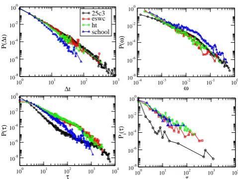
The heterogeneity and burstiness of the contact pat-terns of the face-to-face interactions [10] are revealed by the study of the distribution of the duration ∆t of con-tacts between pairs of agents,P(∆t), the distribution of the total time in contact of pairs of agents (the weight distributionP(ω)), and the distribution of gap times,τ, between two consecutive conversations involving a com-mon individual and two other different agents, for a single agent i, Pi(τ), or considering all the agents, P(τ). All these distributions are heavy-tailed, typically compatible with power-law behaviors (see Fig. 1), corresponding to the burstiness of human interactions [41].

As noted above, diffusion processes such as random walks are moreover particularly impacted by the struc-ture of paths between nodes. In this respect, time re-specting paths represent a crucial feature of any temporal

100 101 102 103

∆t

10-8 10-6 10-4 10-2 100

P(

∆

t)

25c3 eswc ht school

10-4 10-3 10-2 10-1 100

ω

10-8 10-6 10-4 10-2 100

P(

ω)

100 101 102 103 104

τ

10-8 10-6 10-4 10-2 100

P(

τ)

100 101 102 103 104

τ

10-8 10-6 10-4 10-2 100

Pi

(

τ

)

Figure 1. (Color Online) Distributions ofP(∆t) (duration of

contacts),P(ω) (total contact time between pairs of agents),

Pi(τ) (gap times of a single individual i) andP(τ) (global

gap times). In the case ofPi(τ), we only plot the gap times

distribution of the agent which engages in the largest number of conversation, but the other agents exhibit a similar behav-ior. All distributions are heavy-tailed, indicating the bursty nature of face-to-face interactions, for the four empirical con-tact sequences considered.

network, since they determine the set of possible causal interactions between the actors of the graph.

For each (ordered) pair of nodes (i, j), time-respecting paths fromi to j can either exist or not; moreover, the concept of shortest path on static networks (i.e., the path with the minimum number of links between two nodes) yields several possible generalizations in a temporal net-work:

• the fastest path is the one that allows to go from

i to j, starting from the dataset initial time, in the minimum possible time, independently of the number of intermediate steps;

• theshortesttime-respecting path betweeniandjis the one that corresponds to the smallest number of intermediate steps, independently of the time spent between the start fromi and the arrival toj.

For each node pair (i, j), we denote by l_ijf, ls,temp_ij ,

ls,stat_ij the lengths (in terms of the number of hops) respec-tively of the fastest path, the shortest time-respecting path, and the shortest path on the aggregated network, and by ∆tf_ij and ∆ts

ij the duration of the fastest and shortest time-respecting paths, where we take as initial time the first appearance ofiin the dataset. As already noted in other works [21, 43],lf_ij can be much larger than

ls,stat_ij . Moreover, it is clear that lf_ij ≥ l_ijs,temp ≥ls,stat_ij ;

Dataset le hlsi h∆tsi hlfi h∆tfi hls,stati

25c3 0.91 1.67 1607 4.7 893 1.67

eswc 0.99 1.75 884 4.95 287 1.73

ht 0.99 1.67 1157 3.86 452 1.66

school 1 1.76 853 8.27 349 1.73

Table II. (Color Online) Average properties of the shortest time-respecting paths, fastest paths and shortest paths in the projected network, in the datasets considered.

∆ts ij.

We therefore define the following quantities:

• le: fraction of theN(N−1) ordered pairs of nodes for which a time-respecting path exists;

• hlsi: average length (in terms of number of hops along network links) of the shortest time-respecting paths;

• h∆tsi: average duration of the shortest time-respecting paths;

• hlfi: average length of the fastest time-respecting paths;

• h∆tfi: average duration of the fastest time-respecting paths;

• hls,stati: average shortest path length in the binary (static) projected network;

The corresponding empirical values are reported in Ta-ble II. It turns out that the great majority of pairs of nodes are causally connected by at least one path in all datasets. Hence, almost every node can potentially be influenced by any other actor during the time evolution, i.e., the set of sources and the set of influence of the great majority of the elements are almost complete (of sizeN) in all of the considered datasets.

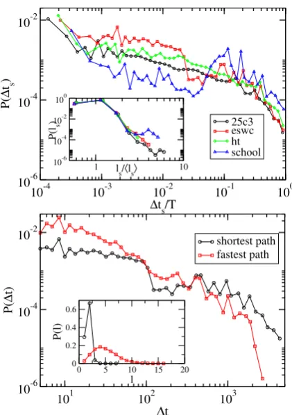
In Fig. 2 we show the distributions of the lengths,

P(ls), and durations, P(∆ts), of the shortest time-respecting path for different datasets. In the same Fig-ure we choose one dataset to compare the P(ls) and the P(∆ts) distributions with the distributions of the lengths, P(lf), and durations, P(∆tf), of the fastest path. The P(ls) distribution is short tailed and peaked on l = 2, with a small average value hlsi, even consid-ering the relatively small sizes N of the datasets, and it is very similar to the projected network one hls,stati (see Table II). The P(lf) distribution, on the contrary, shows a smooth behavior, with an average value hlfi several times bigger than the shortest path one, hlsi, as expected [21, 43]. Note that, despite the important differences in the datasets characteristics, the P(ls) dis-tributions (as well as P(lf), although not shown) col-lapse, once rescaled. On the other hand, theP(∆ts) and P(∆tf) distributions show the same broad-tailed behav-ior, but the average durationh∆tsiof the shortest paths

10-4 10-3 10-2 10-1 100

∆t s/T 10-6

10-4 10-2

P(

∆

t s

)

25c3 eswc ht school

1 l_s/〈l_s〉 10 10-6

10-4 10-2 100

P(l

s

)

101 102 103

∆t

10-6 10-4 10-2

P(

∆

t)

shortest path fastest path

0 5 10 15 20

l

0 0.2 0.4 0.6

P(l)

Figure 2. (Color Online) Top: Distribution of the temporal duration of the shortest time-respecting paths, normalized by

its maximum valueT. Inset: probability distributionP(ls) of

the shortest path length measured over time-respecting paths,

and normalized with its mean valuehlsi. Note that the

dif-ferent datasets collapse. Bottom: Probability distribution of

the duration of the shortestP(∆ts) and fastestP(∆tf)

time-respecting paths, for the eswc dataset. Inset: Probability

dis-tribution of the shortestP(ls) and fastestP(lf) path length

for the same dataset.

is much longer than the average duration h∆tfi of the fastest paths, and of the same order of magnitude than the total duration of the contact sequenceT.

Thus, a temporal network may be topologically well connected and at the same time difficult to navigate or search. Indeed spreading and searching processes need to follow paths whose properties are determined by the temporal dynamics of the network, and that might be either very long or very slow.

C. Synthetic extensions of empirical contact

sequences

im-portant in processes that reach a steady state, such as random walks. As discussed in Sec. II, a walker does not move at every time step, but only with a probability p, and the effective number of movements of a walker is of the order T p. For the considered empirical sequences, this means that the ratio between the number of hops of the walker and the network size, T p/N, assumes val-ues between 3.01 for the school case and 1.60 for the eswc case. Typically, for a random walk processes such small times permit to observe transient effects only, but not a stationary behavior. Therefore we will first explore the asymptotic properties of random walks in syntheti-cally extended contact sequences, and we will consider the corresponding finite time effects in Sec. VI. The syn-thetic extensions preserve at different levels the statistical properties observed in the real data, thus providing null models of dynamical networks.

Inspired by previous approaches to the synthetic ex-tension of empirical contact sequences [1, 7, 13, 22, 44], we consider the following procedures:

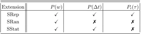
• SRep: Sequence replication. The contact sequence is repeated periodically, defining a new extended characteristic function such that χSRep

e (i, j, t) = χ(i, j, tmodT). This extension preserves all of the statistical properties of the empirical data (obvi-ously, when properly rescaled to take into account the different durations of the extended and empiri-cal time series), introducing only small corrections, at the topological level, on the distribution of time respecting paths and the associated sets of influ-ence of each node. Indeed, a contact present at time t will be again available to a dynamical pro-cess starting at timet0> tafter a timet+T.

• SRan: Sequence randomization. The time order-ing of the interactions is randomized, by construct-ing a new characteristic function such that, at each time step t, χSRan_e (i, j, t) = χ(i, j, t0) ∀i and ∀j, wheret0is a time chosen uniformly at random from the set{1,2, . . . , T}. This form of extension yields at each time step an empirical instantaneous net-work of interactions, and preserves on average all the characteristics of the projected weighted net-work, but destroys the temporal correlations of suc-cessive contacts, leading to Poisson distributions forP(∆t) andPi(τ).

• SStat: Statistically extended sequence. An

inter-mediate level of randomization can be achieved by generating a synthetic contact sequence as follows: we consider the set of all conversations c(i, j,∆t) in the sequence, defined as a series of consecutive contacts of length ∆t between the pair of agentsi

andj. The new sequence is generated, at each time stept, by choosingnconversations (nbeing the av-erage number of new conversations starting at each time step in the original sequence, see Table I), ran-domly selected from the set of conversations, and

100 101 102 103

∆_t

10-8

10-6

10-4

10-2

100

P(

∆

t)

100 101 102 103 104

τ

10-8 10-6 10-4 10-2 100

Pi

(

τ

)

SRep SRan SStat

100 101 102 103 104 105

τ

10-12 10-10 10-8 10-6 10-4 10-2 100

P(

τ

)

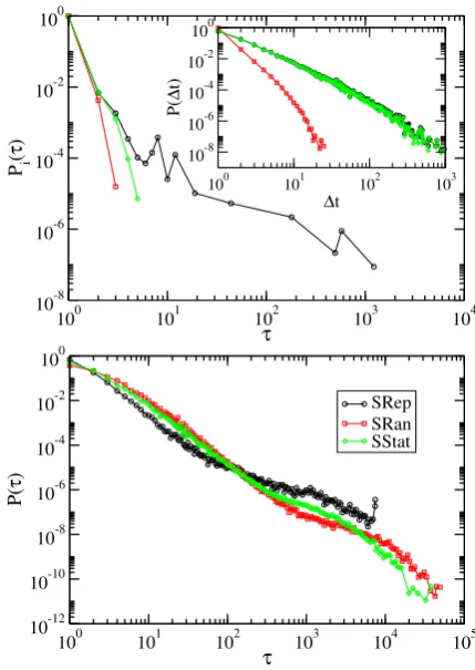
Figure 3. (Color Online) Top: Probability distributionPi(τ)

of a single individual andP(∆t) (inset) for the extended

con-tact sequences SRep, SRan and SStat, for the 25c3 dataset.

The weight distributionP(w) of the original contact sequence

is preserved for every extension. Bottom: Probability

distri-bution of gap timesP(τ) for all the agents in the SRep, SRan

and SStat extensions of the 25c3 dataset.

considering them as starting at timet and ending at time t+ ∆t, where ∆t is the duration of the corresponding conversation. In this procedure we avoid choosing conversations between agentsiand

jwhich are already engaged in a contact started at a previous timet0< t. This extension preserves all the statistical properties of the empirical contact sequence, with the exception of the distribution of time gaps between consecutive conversations of a single individual,Pi(τ).

Extension P(w) P(∆t) Pi(τ)

SRep X X X

SRan X 7 7

SStat X X 7

Table III. Comparison of the properties of the original contact sequence preserved in the synthetic extensions.

the fact that the respective individual burstiness Pi(τ) are bounded, see Fig. 3. This fact can be easily under-stood by considering thatP(τ) can be written in terms of a convolution of the individual gap distributions times the probability of starting a conversation. In the case of SRan extension, the probabilityri that an agentistarts a new conversation is proportional to its strengthsi, i.e. ri=si/(Nhsi). Therefore, the probability that it starts a conversationτtime steps after the last one (its gap distri-bution) is given byPi(τ) =ri[1−ri]τ−1'riexp(−τ ri), for sufficiently small ri. The gap distribution for all agentsP(τ) is thus given by the convolution

P(τ) =

Z

P(s) s

Nhsiexp

−τ s Nhsi

ds, (9)

whereP(s) is the strength distribution. This distribution has an exponential form, which leads, from Eq. (9), to a total gap distributionP(τ)∼(1 +τ /N)−2_{, with a heavy} tail. Analogous arguments can be used in the case of the SStat extension.

IV. RANDOM WALKS ON EXTENDED

CONTACT SEQUENCES

Let us consider a random walk on the sequence of in-stantaneous networks at discrete time steps, which is equivalent to a message passing strategy in which the message is passed to a randomly chosen neighbor. The walker present at node i at time t hops to one of its neighbors, randomly chosen from the set of vertices

Vi(t) ={j|χ(i, j, t) = 1}, (10)

of which there is a number

ki(t) =

X

j

χ(i, j, t), (11)

If the node i is isolated at time t, i.e. Vi(t) = ∅, the walker remains at nodei. In any case, time is increased

t→t+ 1.

Analytical considerations analogous to those in Sec. II for the case of contact sequences are hampered by the presence of time correlations between contacts. In fact, as we have seen, the contacts between a given pair of agents are neither fixed nor completely random, but in-stead show long range temporal correlations. An excep-tion is represented by the randomized SRan extension,

in which successive contacts are by construction uncor-related. Considering that the random walker is in vertex

i at time t, at a subsequent time step it will be able to jump to a vertexj whenever a connection betweeni

andj is created, and a connection betweeni andj will be chosen with probability proportional to the number of connections between i and j in the original contact sequence, i.e. proportional to ωij. That is, a random walk on the extended SRan sequence behaves essentially as in the corresponding weighted projected network, and therefore the equations obtained in Sec. II, namely

τi= hsiN

si

, (12)

and

C(t)

N = 1−

1

N

X

i exp

−t si hsiN

(13)

apply. In this last expression for the coverage we can approximate the sum by an integral, i.e.

C(t)

N = 1−

Z

dsP(s) exp

−t s hsiN

, (14)

being P(s) the distribution of strengths. Giving that

P(s) has an exponential behavior, we can obtain from the last expression

C(t)

N '1−

1 + t

N

−1

. (15)

V. NUMERICAL SIMULATIONS

In this Section we present numerical results from the simulation of random walks on the extended contact se-quences described above. Measuring the coverageC(t) we set the duration of these sequences to 50 times the duration of the original contact sequence T, while to evaluate the MFPT between two nodesi and j, τij, we let the RW explore the network up to a maximum time

tmax = 108. Each result we report is averaged over at least 103 _{independent runs.}

A. Network exploration

10-4 10-2 100 102 10-6

10-4 10-2 100

C(t)/N

SRep SRan SStat th. pred.

10-4 10-2 100 102 104

10-4 10-3 10-2 10-1 100

10-4 10-2 100 102 104

pt/N

10-4 10-3 10-2 10-1 100

10-4 10-2 100 102

10-4 10-3 10-2 10-1 100

25c3 eswc

ht school

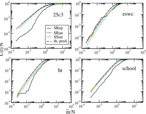
Figure 4. (Color Online) Normalized coverage C(t)/N as a

function of the rescaled time pt/N, for the SRep, SRan and

SStat extension of empirical data. The numerical evaluation of Eq. (13) is shown as a dashed line, and each panel in the figure corresponds to one of the empirical datasets considered. The exploration of the empirical repeated data sets (SRep) is slower than the other cases. Moreover, the SRan is in agree-ment with the theoretical prediction, and the SStat case shows a close (but systematically slower) behavior. This indicates that the main slowing down factor in the SRep sequence is represented by the irregular distribution of the interactions in time, whose contribution is eliminated in the randomized sequences.

in the original contact sequence, for the SStat extension we obtain numerically different values ofp, which we use when rescaling time in the corresponding simulations.

The coverage corresponding to the SRan extension is very well fitted by a numerical simulation of Eq. (15), which predicts the coverageC(t)/N obtained in the cor-respondent projected weighted network. Moreover, when using the rescaled timept, the SRan coverages for differ-ent datasets collapse on top of each other for small times, with a linear time dependenceC(t)/N ∼t/N fortN

as expected in static networks, showing a universal be-havior (not shown).

The coverage obtained on the SStat extension is sys-tematically smaller than in the SRan case, but follows a similar evolution. On the other hand, the RW explo-ration obtained with the SRep prescription is generally slower than the other two, particularly for the 25c3 and ht datasets. As discussed before, the original contact sequence, as well as the SRep extension, are character-ized by irregular distributions of the interactions in time, showing periods with few interacting nodes and corre-spondingly a small number n(t) of new started conver-sations, followed by peaks with many interactions (see Fig. 5). This feature slows down the RW exploration, because the RW may remain trapped for long times on

0 500 1000 1500 2000

t 0

20 40 60 80 100

n(t)

Figure 5. (Color Online) Number of new conversationsn(t)

started per unit time in the SRep (black, full dots), SRan (red, empty squares) and SStat (green, diamonds) extensions of the school dataset.

isolated nodes. The SRan and the SStat extensions, on the contrary, both destroy this kind of temporal struc-ture, balancing the periods of low and high activity: the SRan extension randomizes the time order of the contact sequence, and the SStat extension evens the number of interacting nodes, with n new conversations starting at each time step.

The similarity between the random walk processes on the SRan and SStat dynamical networks shows that the random walk coverage is not very sensitive to the het-erogenous durations of the conversations, as the main difference between these two cases is thatP(∆t) is nar-row for SRan and broad for SStat. In these cases, the ob-served behavior is instead well accounted for by Eq. (13), taking into account only the weight distribution of the projected network, i.e., the heterogeneity between aggre-gated conversation durations. Therefore, the slower ex-ploration properties of the SRep sequences can be mostly attributed to the correlations between consecutive con-versations of the single individuals, as given by the indi-vidual gap distributionPi(τ), (see [13, 15, 22] for analo-gous results in the context of epidemic spreading).

A remark is in order for the 25c3 conference. A close inspection of Fig. 4 shows that the RW does not reach the whole network in any of the extensions schemes, with

100 101 102

1 + pt/N

10-5

10-4

10-3

10-2

10-1

100

1 - C(t)/N

25c3 eswc ht school

(1+ptN)-1

0 50 100 150

ptN 10-4

10-2 100

1-C(t)/N

100 101 102

1+pt/N

10-5

10-4

10-3

10-2

10-1

100

1-C(t)/N 25c3eswc

ht school MF pred.

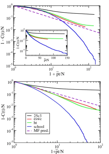
Figure 6. (Color Online) Asymptotic residual coverage 1−

C(t)/N as a function of ¯pt/N for the SRep (top) and SRan

(bottom) extended sequences, for different datasets.

value limt→∞CN(t) = 1. Indeed, the mean-field calcu-lations presented in Secs. II and III C suggest a power-law decay with (1 + ¯pt/N)−1 _{for the residual coverage} 1−C(t)/N. In Fig. 6 we plot the asymptotic coverage for large times in the 4 datasets considered. We can see that RW on the eswc and ht dataset conform at large times quite reasonably to the expected theoretical prediction in Eq. (15), both for the SRep and SRan extensions. The 25c3 dataset shows, as discussed above, a considerable slowing down, with a very slow decay in time. Interest-ingly, the school dataset is much faster than all the rest, with a decay of the residual coverage 1−C(t)/N exhibit-ing an approximate exponential decay. It is noteworthy that the plots for the randomized SRan sequence do not always obey the mean-field prediction (see lower plot in Fig. 6). This deviation can be attributed to the fact that SRan extensions preserve the topological structure of the projected weighted network, and it is known that, in some instances, random walks on weighted networks can deviate from the mean-field predictions [45]. These deviations are particularly strong in the case of the 25c3 dataset, where connections with a very small weight are present.

10-6 10-4 10-2

100 102 104 106

108 _SRep

SRan SStat MF pred.

10-4 10-2

100 102 104 106

10-5 10-4 10-3 10-2 10-1

s_i/(N〈s〉)

100 102 104 106

p

τ i

10-4 10-3 10-2 10-1

101 102 103 104 105

ht

25c3 eswc

school

Figure 7. (Color Online) Rescaled mean first passage time

τi, shown against the strengthsi, normalized with the total

strengthNhsi, for the SRep, SRan and SStat extensions of

empirical data. The dashed line represents the prediction of Eq. (12). Each panel in the figure corresponds to one of the empirical datasets considered.

B. Mean first-passage time

Let us now focus on another important characteristic property of random walk processes, namely the MFPT defined in Section II. Figure 7 shows the correlation be-tween the MFPT τi of each node, measured in units of rescaled timept, and its normalized strengthsi/(Nhsi). The random walks performed on the SRan and SStat extensions are very well fitted by the mean field theory, i.e. Eq. (12) (predicting thatτi is inversely proportional to si), for every dataset considered; on the other hand, random walks on the extended sequence SRep yield at the same time deviations from the mean-field prediction and much stronger fluctuations around an average behav-ior. Figure 8 addresses this case in more detail, showing that the data corresponding to RW on different datasets collapse on an average behavior that can be fitted by a scaling function of the form

τi∼ 1

p×

_s

i Nhsi

−α

, (16)

with an exponentα'0.75.

10-6 10-4 10-2 100

s_i/(N〈s〉)

100

102

104

106

p

τ i

25c3 eswc ht school

slope α=−0.75

slope α=−1

Figure 8. (Color Online) Mean first passage time at nodei,

in units of rescaled timept, vs. the strength si, normalized

with the total strengthNhsi, for RW processes on the SRep

datasets extension. All data collapse close to the continuous

line whose slope, α'0.75, differs from the theoretical one,

α= 1.0, shown as a dashed line.

searching process in the empirical, correlated, network is slower than in the randomized versions, in agreement with the smaller coverage observed in Fig. 4.

The data collapse observed in Fig. 8 for the SRep case leads to two noticeable conclusions. First, although the various datasets studied correspond to different con-texts, with different numbers of individuals and densities of contacts, simple rescaling procedures are enough to compare the processes occurring on the different tempo-ral networks, at least for some given quantities. Second, the MFPT at a node is largely determined by its strength. This can indeed seem counterintuitive as the strength is an aggregated quantity (that may include contact events occurring at late times). However, it can be rationalized by observing that a large strength means a large num-ber of contacts and therefore a large probability to be reached by the random walker. Moreover, the fact that the strength of a node is an aggregate view of contact events that do not occur homogeneously for all nodes but in a bursty fashion leads to strong fluctuations around the average behavior, which implies that nodes with the same strength can also have rather different MFPT (Note the logarithmic scale on the y-axis).

VI. RANDOM WALKS ON FINITE CONTACT

SEQUENCES

The case of finite sequences is interesting from the point of view of realistic searching processes. The limited duration of a human gathering, for example, imposes a constraint on the length of any searching strategy. Fig.

0 1 2 3 4

pt/N 0.0

0.1 0.2 0.3 0.4 0.5

C(t)/N

25c3 eswc ht school

100 102 _∆t 104

new 10-8

10-6 10-4 10-2 100

P(

∆

tnew

)

Figure 9. (Color Online) Normalized coverage C(t)/N as

function of the rescaled timept/N for the different datasets.

The inset shows the probability distributionP(∆tnew) of the

time lag ∆tnew between the discovery of two new vertices.

Only the discovery of the first 5% of the network is consid-ered, to avoid finite size effects [46].

9 shows the normalized C(t)/N coverage as a function of the rescaled timept/N. The coverage exhibits a con-siderable variability in the different datasets, which do not obey the rescaling obtained for the extended SRan and SStat sequence. The probability distribution of the time lags ∆tnew between the discovery of two new ver-tices [46] provides further evidence of the slowing down of diffusion in temporal networks. The inset of Fig. 9 indeed shows broad tailed distributionsP(∆tnew) for all the dataset considered, differently from the exponential decay observed in binary static networks [46].

The important differences in the rescaled coverage

C(t)/N between the various datasets, shown in Fig. 9, can be attributed to the choice of the time scale,pt/N, which corresponds to a temporal rescaling by an aver-age quantity. We can argue, indeed, that the speed with which new nodes are found by the RW is propor-tional to the number of new conversations n(t) started at each time step t, thus in the RW exploration of the temporal network the effective time scale is given by the integrated number of new conversations up to time t,

N(t) =Rt

0n(t

0_)dt0_{. In Fig. 10 we display the correlation}

between the coverage C(t)/N and the number of new conversations realized up to timet,N(t), normalized for the mean number of new conversations per unit of time,

n. While the relation is not strictly linear, a very strong positive correlation appears between the two quantities. The complex pattern shown by the average coverage

10-2 10-1 100 101 102 103 104 N(t)/ n

10-4 10-2 100

C(t)/N

25c3 escw ht school

α=1

Figure 10. (Color Online) CoverageC(t)/N as a function of

the number of new conversation realized up to time t,

nor-malized for the mean number of new conversation per unit of

time,n, for different datasets.

0 100 200 300 400 500 600 rank

0 0.1 0.2 0.3 0.4

Ci

(

∆

T)

25c3 eswc ht school

0 100 200 300 400 500 600

rank 0

0.2 0.4 0.6 0.8 1

Ci

(T)

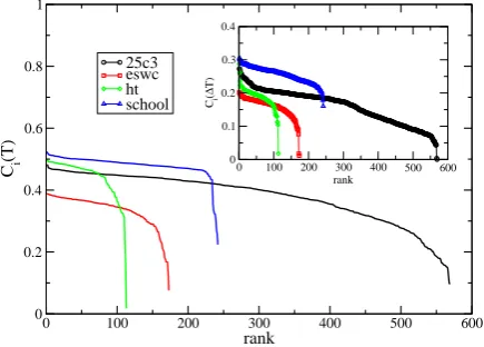
Figure 11. (Color Online) Rank plot of the coverage Ci

ob-tained starting from nodeiin the contact sequence of duration

T, averaged over 103 _{runs. In the inset, we show a rank plot}

of the coverageCi(∆T) up to a fixed time ∆T= 103.

all vertices are equivalent. A first explanation of the vari-ability inCicomes from the fact that not all nodes appear simultaneously on the network at time 0. Ift0,i denotes the arrival time of nodei in the system, a random walk starting fromiis restricted toT_ir=T−t0,i: nodes arriv-ing at later times have less possibilities to explore their set of influence, even if this set includes all nodes. To put all nodes on equal footing and compensate for this somehow trivial difference between nodes, we consider the coverage of random walkers starting on the different verticesiand walking for exactly ∆Ttime steps (we limit of course the study to nodes with t0,i < T−∆T).

Dif-10-4 10-3 10-2 10-1 100 101 102

pTs_i/〈s〉N

10-4 10-3 10-2 10-1 100

Pr

(i)

25c3 eswc ht school MF pred.

0 pTs_i/〈s〉N 10

0,0 0,5 1,0

P r

(i)

25c3 eswc ht school MF pred.

Figure 12. (Color Online) Correlation between the

probabil-ity of nodeito be reached by the RW,Pr(i), and the rescaled

strength pT si/Nhsi for different datasets. The curves

ob-tained by different dataset collapse, but they do not follow the mean-field behavior predicted by of Equation (17) (dashed line). The inset shows the same data on a linear scale, to em-phasize the deviation from mean-field.

ferences in the coverageCi(∆T) will then depend on the intrinsic properties of the dynamic network. For a static network indeed, either binary or weighted, the coverage

Ci(∆T) would be independent of i, as random walkers on static networks lose the memory of their initial posi-tion in a few steps, reaching very fast the steady state behavior Eq. (3). As the inset of Fig. 11 shows, impor-tant heterogeneities are instead observed in the coverage of random walkers starting from different nodes on the dynamic network, even if the random walk duration is the same.

Another interesting quantity is the probability that a vertexiis discovered by the random walker. As discussed in Section II, at the mean field level the probability that a nodei is visited by the RW at any time less than or equal tot(the random walk reachability) takes the form

Pr(i;t) = 1−exp[−tρ(i)]. Thus the probability that the nodeiis reached by the RW at any time in the contact sequence is

Pr(i) = 1−exp

−pT si Nhsi

, (17)

10-4 10-2 100 102

pTs_i/2〈s〉N

10-4

10-2

100

Pr

(i)

10

pTs_i/2〈s〉N

0,5 1,0

Pr

(i)

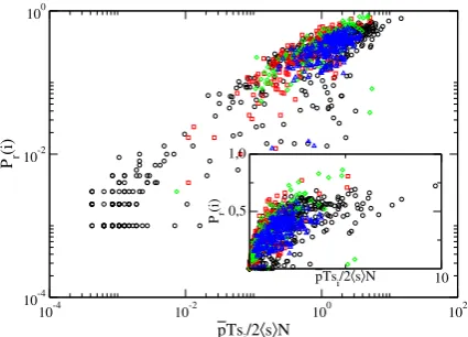
Figure 13. (Color Online) Correlation between the probability

of nodei to be reached by a RW of lengthT /2, Pr(i), and

the rescaled strengthpT si/Nhsifor different datasets, where

si is computed on the whole dataset of length T. The inset

shows the same data on a linear scale.

sequences, the dynamical property Pr(i) can be in part “predicted” by an aggregate quantity such as si. Strong deviations from the mean-field prediction of Eq. (17) are however observed, with a tendency of Pr(i) to saturate at large strengths to values much smaller than the ones obtained on a static network. Thus, although the set of sources of almost every node i has size N, as shown in Sec. III B (i.e., there exists a time respecting path between almost every possible starting point of the RW processes and every target node i), the probability for nodeito be effectively reached by a RW is far from being equal to 1.

Moreover, rather strong fluctuations ofPr(i) at given si are also observed: si is indeed an aggregate view of contacts which are typically inhomogeneous in time, with bursty behaviors2 _{. Figure 13 also shows that the} reachability computed at shorter time (hereT /2) displays stronger fluctuations as a function of the strengthsi com-puted on the whole time sequence: Pr(i) for shorter RW is naturally less correlated with an aggregate view which takes into account a more global behavior ofi.

VII. DISCUSSION AND CONCLUSIONS

In this paper we have investigated the behavior of ran-dom walks on temporal networks. In particular, we have focused on real face-to-face contact networks concerning four different datasets. These dynamical networks ex-hibit heterogeneous and bursty behavior, indicated by

2 _{When considering RW on a contact sequence of length T} ran-domized according to the SRan procedure instead, Eq. (17) is well obeyed and only small fluctuations ofPr(i) are observed at

a fixedsi(not shown).

the long tailed distributions for the lengths and strength of conversations, as well as for the gaps separating suc-cessive interactions. We have underlined the importance of considering not only the existence of time preserving paths between pairs of nodes, but also their temporal du-ration: shortest paths can take much longer than fastest paths, while fastest paths can correspond to many more hops than shortest paths. Interestingly, the appropriate rescaling of these quantities identifies universal behaviors shared across the four datasets.

Given the finite life-time of each network, we have con-sidered as substrate for the random walk process the replicated sequences in which the same time series of contact patterns is indefinitely repeated. At the same time, we have proposed two different randomization pro-cedures to investigate the effects of correlations in the real dataset. The “sequence randomization” (SRan) de-stroys any temporal correlation by randomizing the time ordering of the sequence. This allows to write down ex-act mean-field equations for the random walker explor-ing these networks, which turn out to be substantially equivalent to the ones describing the exploration of the weighted projected network. The “statistically extended sequence” (SStat), on the other hand, selects random conversations from the original sequence, thus preserv-ing the statistical properties of the original time series, with the exception of the distribution of time gaps be-tween consecutive conversations.

We have performed numerical analysis both for the coverage and the MFPT properties of the random walker. In both cases we have found that the empirical sequences deviate systematically from the mean field prediction, in-ducing a slowing down of the network exploration and of the MFPT. Remarkably, the analysis of the random-ized sequences has allowed us to point out that this is due uniquely to the temporal correlations between con-secutive conversations present in the data, and not to the heterogeneity of their lengths. Finally, we have ad-dressed the role of the finite size of the empirical net-works, which turns out to prevent a full exploration of the random walker, though differences exist across the four considered cases. In this context, we have also shown that different starting nodes provide on average different coverages of the networks, at odds to what happens in static graphs. In the same way, the probability that the nodeiis reached by the RW at any time in the contact sequence exhibits a common behavior across the differ-ent time series, but it is not described by the mean-field predictions for the aggregated network, which predict a faster process.

observed dynamics, and that will represent a reference for the understanding of more complex diffusive dynam-ics occurring on dynamic networks. Our investigations also open interesting directions for future work. For in-stance, it would be interesting to investigate how random walks starting from different nodes explore first their own neighborhood [47], which might lead to hints about the definition of “temporal communities” (see e.g. [48] for an algorithm using RW on static networks for the detec-tion of static communities); various measures of nodes centrality have also been defined in temporal networks [1, 44, 49–51], but their computation is rather heavy, and RW processes might present interesting alternatives,

sim-ilarly to the case of static networks [52].

ACKNOWLEDGMENTS

We thank the SocioPatterns collaboration

(www.sociopatterns.org) for providing privileged access to dynamical network data. M.S., R.P.-S. and A. Baronchelli acknowledge financial support from the Spanish MEC (FEDER), under project FIS2010-21781-C02-01, and the Junta de Andaluc´ıa, under project No. P09-FQM4682.. R.P.-S. acknowledges additional support through ICREA Academia, funded by the Generalitat de Catalunya.

[1] P. Holme and J. Saram¨aki, “Temporal networks,”

(2011), eprint arxiv:1108.1780v1.

[2] S. Wasserman and K. Faust, Social Network Analysis:

Methods and Applications (Cambridge University Press, Cambridge, 1994).

[3] M. E. J. Newman, Proc. Natl. Acad. Sci. USA 98, 404

(2001).

[4] A.-L. Barab´asi and R. Albert, Science286, 509 (1999).

[5] A. Barrat, M. Barth´elemy, and A. Vespignani,

Dynami-cal processes on complex networks (Cambridge, 2008). [6] P. Hui, A. Chaintreau, J. Scott, R. Gass, J. Crowcroft,

and C. Diot, in WDTN ’05: Proceedings of the 2005

ACM SIGCOMM workshop on Delay-tolerant

network-ing (ACM, New York, NY, USA, 2005) pp. 244–251.

[7] P. Holme, Phys. Rev. E71, 046119 (2005).

[8] J.-P. Onnela, J. Saram¨aki, J. Hyv¨onen, G. Szab´o,

D. Lazer, K. Kaski, J. Kert´esz, and A.-L. Barab´asi,

Pro-ceedings of the National Academy of Sciences104, 7332

(2007).

[9] A. Gautreau, A. Barrat, and M. Barth´elemy,

Proceed-ings of the National Academy of Sciences 106, 8847

(2009).

[10] C. Cattuto, W. Van den Broeck, A. Barrat, V. Colizza,

J.-F. Pinton, and A. Vespignani, PLoS ONE 5, e11596

(2010).

[11] J. Tang, S. Scellato, M. Musolesi, C. Mascolo, and V.

La-tora, Phys. Rev. E 81, 055101 (2010).

[12] P. Bajardi, A. Barrat, F. Natale, L. Savini, and V.

Col-izza, PLoS ONE6, e19869 (2011).

[13] J. Stehl´e, N. Voirin, A. Barrat, C. Cattuto, V. Colizza,

L. Isella, C. R´egis, J.-F. Pinton, N. Khanafer, W. Van den

Broeck, and P. Vanhems, BMC Medicine9(2011).

[14] G. Miritello, E. Moro, and R. Lara, Phys. Rev. E 83,

045102 (2011).

[15] M. Karsai, M. Kivel¨a, R. K. Pan, K. Kaski, J. Kert´esz,

A.-L. Barab´asi, and J. Saram¨aki, Phys. Rev. E 83,

025102 (2011).

[16] A. Scherrer, P. Borgnat, E. Fleury, J.-L. Guillaume, and

C. Robardet, Comp. Net. 52, 2842 (2008).

[17] S. Hill and D. Braha, Phys. Rev. E82, 046105 (2010).

[18] J. Stehl´e, A. Barrat, and G. Bianconi, Phys. Rev. E81,

035101 (2010).

[19] K. Zhao, J. Stehl´e, G. Bianconi, and A. Barrat, Phys.

Rev. E 83, 056109 (2011).

[20] L. E. C. Rocha, F. Liljeros, and P. Holme, PLoS Comput

Biol7, e1001109 (2011).

[21] L. Isella, J. Stehl´e, A. Barrat, C. Cattuto, J.-F. Pinton,

and W. V. den Broeck, J. Theor. Biol271, 166 (2011).

[22] M. Kivela, R. Kumar Pan, K. Kaski, J. Kertesz,

J. Saramaki, and M. Karsai, “Multiscale analysis of

spreading in a large communication network,” (2011),

arXiv:1112.4312v1.

[23] N. Fujiwara, J. Kurths, and A. D´ıaz-Guilera, Physical

Review E83, 025101 (2011).

[24] R. Parshani, M. Dickison, R. Cohen, H. E. Stanley, and

S. Havlin, EPL (Europhysics Letters)90, 38004 (2010).

[25] A. Baronchelli and A. D´ıaz-Guilera, Phys. Rev. E 85,

016113 (2012).

[26] G. H. Weiss, Aspects and Applications of the

Ran-dom Walk (North-Holland Publishing Co., Amsterdam, 1994).

[27] B. Hughes, Random walks and random environments

(Clarendon Press, Oxford (UK), 1995).

[28] L. Lov´asz, inCombinatorics, Paul Erd¨os is Eighty(J´anos

Bolyai Mathematical Society, Budapest, 1996) p. 353. [29] L. A. Adamic, R. M. Lukose, A. R. Puniyani, and B. A.

Huberman, Phys. Rev. E64, 046135 (2001).

[30] Q. Lv, P. Cao, E. Cohen, K. Li, and S. Shenker, in

Proceedings of the 16th international conference on Su-percomputing (ACM Press, New York, NY, USA, 2002) pp. 84–95.

[31]http://www.sociopatterns.org/.

[32] A. Barrat, M. Barth´elemy, R. Pastor-Satorras, and

A. Vespignani, Proc. Natl. Acad. Sci. USA 101, 3747

(2004).

[33] J. D. Noh and H. Rieger, Phys. Rev. Lett. 92, 118701

(2004).

[34] A.-C. Wu, X.-J. Xu, Z.-X. Wu, and Y.-H. Wang, Chin.

Phys. Lett.24, 577 (2007).

[35] D. Stauffer and M. Sahimi, Phys. Rev. E 72, 46128

(2005).

[36] E. Almaas, R. V. Kulkarni, and Stroud, Phys. Rev. E

68, 056105 (2003).

[37] M. E. J. Newman, Networks: An introduction (Oxford

University Press, Oxford, 2010).

[38] J. Stehl´e, N. Voirin, A. Barrat, C. Cattuto, L. Isella,

J.-F. Pinton, M. Quaggiotto, W. Van den Broeck, C. R´egis,

[39] V. Kostakos, Physica A: Statistical Mechanics and its

Applications388, 1007 (2009).

[40] V. Nicosia, J. Tang, M. Musolesi, G. Russo, C. Mascolo, and V. Latora, arXiv:1106.2134 (2011).

[41] A. Barab´asi, Nature435, 207 (2005).

[42] W. V. den Broeck, C. Cattuto, A. Barrat, M. Szomsor,

G. Correndo, and H. Alani, inProceedings of the 8th

An-nual IEEE International Conference on Pervasive Com-puting and Communications (2010) p. 226.

[43] G. Kossinets, J. Kleinberg, and D. Watts, inProceedings

of the 14thACM SIGKDD International Conference on Knowledge Discovery and Data Mining (2008).

[44] R. K. Pan and J. Saram¨aki, Phys. Rev. E 84, 016105

(2011).

[45] A. Baronchelli and R. Pastor-Satorras, Phys. Rev. E82,

011111 (2010).

[46] A. Baronchelli, M. Catanzaro, and R. Pastor-Satorras,

Phys. Rev. E78, 011114 (2008).

[47] A. Baronchelli and V. Loreto, Phys. Rev. E73, 026103

(2006).

[48] P. Pons and M. Latapy, inProceedings of the 20th

Inter-national Symposium on Computer and Information Sci-ences (ISCIS’05), Lecture Notes in Computer Science, Vol. 3733 (Springer, Istanbul, Turkey, 2005) pp. 284–293.

[49] D. Braha and Y. Bar-Yam, inAdaptive Networks,

Under-standing Complex Systems, Vol. 51, edited by T. Gross and H. Sayama (Springer Berlin / Heidelberg, 2009) pp. 39–50.

[50] J. Tang, M. Musolesi, C. Mascolo, V. Latora, and

V. Nicosia, in Proceedings of the 3rd Workshop on

So-cial Network Systems, SNS ’10 (ACM, New York, NY, USA, 2010) pp. 3:1–3:6.

[51] K. Lerman, R. Ghosh, and J. H. Kang, inProceedings

of the Eighth Workshop on Mining and Learning with Graphs, MLG ’10 (ACM, New York, NY, USA, 2010) pp. 70–77.