Uncertainty quantification of power spectrum and spectral
1moments estimates subject to missing data
2Yuanjin Zhang1,Liam Comerford2,Ioannis A. Kougioumtzoglou3
Edoardo Patelli1,Michael Beer124
1Institute for Risk and Uncertainty, University of Liverpool, Liverpool L69 7ZF,
U.K.
2Institute for Risk and Reliability, Leibniz University of Hannover, Hannover,
Ger-many.
3The Fu Foundation School of Engineering and Applied Science, Dept. of Civil
Engineering and Engineering Mechanics, Columbia University, New York, NY
10027.
4School of Civil Engineering & Shanghai Institute of Disaster Prevention and Relief,
Tongji University, China.
3
ABSTRACT 4
In this paper, the challenge of quantifying the uncertainty in stochastic process spectral
5
estimates based on realizations with missing data is addressed. Specifically, relying on
rela-6
tively relaxed assumptions for the missing data and on a Kriging modeling scheme, utilizing
7
fundamental concepts from probability theory, and resorting to a Fourier based
representa-8
tion of stationary stochastic processes, a closed-form expression for the probability density
9
function (PDF) of the power spectrum value corresponding to a specific frequency is derived.
10
Next, the approach is extended for determining the PDF of spectral moments estimates as
11
well. Clearly, this is of significant importance to various reliability assessment methodologies
12
that rely on knowledge of the system response spectral moments for evaluating its survival
13
probability. Further, it is shown that utilizing a Cholesky kind decomposition for the PDF
14
related integrals the computational cost is kept at a minimal level. Several numerical
exam-15
ples are included and compared against pertinent Monte Carlo simulations for demonstrating
the validity of the approach.
17
Keywords: Uncertainty quantification; Survival probability; Spectral moments; Missing
18
data; Kriging; Spectral estimation
19
20
INTRODUCTION 21
In research fields such as stochastic structural dynamics, stochastic processes are most
22
often described by statistical quantities such as the power spectrum. In this regard, several
23
approaches exist in the literature for stochastic process power spectrum estimation. For
24
instance, a Fourier basis is typically utilized in the spectral estimation of stationary processes
25
(Newland 1993). Further, similar to the stationary case, the evolutionary power spectrum
26
related to non-stationary processes can be estimated by employing wavelet (e.g. (Spanos and
27
Failla 2004); (Kougioumtzoglou et al. 2012) ) or chirplet bases (Politis et al. 2007) among
28
other alternatives; see also (Qian 2002) for a detailed presentation of joint time-frequency
29
analysis techniques.
30
It is noted that the above spectral estimation approaches often require a large number
31
of complete data samples for attaining a predefined adequate degree of accuracy. However,
32
missing data in measurements is frequently an unavoidable situation. In fact, missing data
33
are possible in almost any situation where data are collected and stored. Indicative reasons
34
in engineering dynamics measurement applications include failure and/or restricted use of
35
equipment, as well as data corruption and cost/bandwidth limitations.Thus, standard
spec-36
tral analysis techniques that inherently assume the existence of full sets of data, such as
37
those based on Fourier, wavelet and chirplet transforms, cannot be used in a straightforward
38
manner.
39
To address this challenge, a number of signal reconstruction techniques subject to
miss-40
ing/incomplete data (e.g. Lomb-Scargle periodogram, iterative deconvolution method CLEAN,
41
ARMA-model based techniques, etc) have been developed with various degrees of accuracy;
42
see (Wang et al. 2005) for a review. Indicatively, (Comerford et al. 2016) developed recently a
compressive sensing approach (e.g. (Eldar and Kutyniok 2012)) based on L1-norm
minimiza-44
tion for stationary and non-stationary stochastic process/field (evolutionary) power spectrum
45
estimation subject to highly incomplete data, which has already been applied to practical
46
engineering problems (Comerford et al. 2017; Kougioumtzoglou et al. 2017). The approach
47
has been shown to be particularly advantageous for cases where multiple records/realizations
48
compatible with a stochastic process are available. In such cases, a re-weighting procedure
49
can be introduced to improve the result to a large degree (Comerford et al. 2014). Further,
50
an artificial neural network based approach was also developed recently having the advantage
51
that no prior knowledge of the underlying process is required (Comerford et al. 2015a).
52
Although all of the above methodologies can, depending on the setting, potentially
pro-53
vide a relatively accurate stochastic process power spectrum estimate, they will also
prop-54
agate inaccuracies from missing data predictions in the time domain through to the final
55
spectral estimates. Most of the aforementioned techniques estimate the power spectrum
56
by reconstructing missing parts of the data, and based on these reconstructed full data,
57
standard spectral analysis methods are applied. Nevertheless, reconstructing the available
58
records, and thus, deterministically estimating/predicting missing values, rarely accounts for
59
the inherent uncertainty associated with the missing data. Hence, there is merit in
develop-60
ing a methodology for quantifying the uncertainty in a given spectral estimate as a result of
61
the uncertainty related to the missing data in the time/space domain.
62
In this manner, to quantify the uncertainty of spectral estimates subject to missing data,
63
a stochastic model accounting for the uncertainty in the missing data in the time/space
64
domain can be considered based on any available prior knowledge (e.g. an appropriately
65
estimated probability density function (PDF)). Further, the uncertainty in the missing data
66
can be propagated and the PDF for each individual power spectrum point can be determined
67
in the frequency domain. In this regard, (Comerford et al. 2015b) proposed a methodology
68
and determined a closed form expression for the power spectrum estimate PDF under the
69
assumption that the (missing data) variables in the time domain are independent Gaussian
random variables. Note, however, that this approach does not consider the correlation
71
between the missing points, and thus, can be largely unrepresentative, for instance, of a
72
signal with harmonic features. Further, by virtue of the central limit theorem (Billingsley
73
2008), it is reasonable for many cases (e.g. environmental processes such as earthquakes,
74
winds, sea waves and, for linear systems, the structural responses subject to these effects)
75
to consider the missing points following a multi-variate Gaussian PDF.
76
In this paper, the approach developed in (Comerford et al. 2015b) is extended to account
77
for the correlation between the missing data. Although determining the exact correlation
78
between points is practically a quite challenging task, an estimate can be obtained by relying
79
on existing available data and employing various modeling schemes such as Kriging (Stein
80
1999). Further, an additional significant contribution of the herein proposed methodology
81
is that it is generalized to evaluate not only the power spectrum points PDFs, but also
82
the PDFs of the corresponding spectral moments. Clearly, this is of considerable
impor-83
tance to various engineering dynamics applications such as to structural system reliability
84
assessment, where the survival probability (or equivalently, the first-passage time) can be
85
estimated approximately based on knowledge of spectral moments (Vanmarke 1975). Several
86
numerical examples are included and compared against pertinent Monte Carlo simulations
87
for demonstrating the validity of the approach.
88
89
MATHEMATICAL FORMULATION 90
Uncertainty quantification of the power spectrum estimate under missing data 91
Consider a zero mean stationary process represented as
92
f(t) =
Z +∞
−∞
A(ω)eiωtdZ(ω), (1)
93
(Priestley 1982; Cramer and Leadbetter 1967), where A(ω) is a deterministic function and
94
dZ(ω) is a zero mean orthonormal increment stochastic process. The two-sided power
trum Sf(ω) of processf(t) is then defined as Sf(ω) = |A(ω)|2. In general, realizations of a 96
stochastic process that are compatible with a given spectrum can be generated by a spectral
97
representation methodology (Shinozuka and Deodatis 1991) in the form
98
f(t) = 2
N−1 X
n=0 q
Sf(ω)∆ωcos(ωnt+φn), (2)
99
where φn is the independent random phase angle distributed uniformly over the interval
100
[0,2π]. The realizations generated by Eq.(2) exhibit the property of ergodicity (Shinozuka
101
and Deodatis 1991); hence, the power spectrum Sf(ω) of the underlying process can be
102
estimated by utilizing a single realization only. In this regard, and employing the discrete
103
Fourier transform (DFT) yields
104
Sf(ωk) = lim N−→∞
T
2πN2
N−1 X
n=0
xne−2πikn/N 2 , (3) 105
whereN is the number of data points,tandkare the time and frequency indices respectively,
106
and T is the time duration. In the following, the condition N −→ ∞ is omitted, for
107
convenience, under the assumption that the length is long enough to provide with an accurate
108
spectrum estimate. Following the notation of (Comerford et al. 2015b), the data points are
109
divided into 2 parts: the known points xα and missing pointsxβ, where α and β are indices
110
of the known and unknown points, respectively; thus, Eq.(3) can be further cast in the form
111
Sf(ωk) =
T
2πN2|M1 +M2−i(M3+M4)| 2
= T
2πN2
(M1+M2)2+ (M3+M4)2
(4)
112
where M1 =
P
αxαcos 2πkα
N
, M2 =
P
βxβcos 2πkβ
N
, M3 =
P
αxαsin 2πkα
N
, and M4 =
113
P
αxαsin 2πkαN
. Next, Sf(ωk) is rewritten into the simpler form 114
Sf(ωk) = (c1+a0Xβ)2+ (c2+b0Xβ)2 (5)
where (0) denotes the transpose,
116
c1 = r
T
2πN2 X
α
xαcos 2πkα N (6) 117 118
c2 = r
T
2πN2 X
α
xαsin 2πkα N (7) 119 120 a= r T
2πN2
cos
2πkβ1
N
,cos
2πkβ2
N
, ...,cos
2πkβu
N 0 (8) 121 122 b = r T
2πN2
sin
2πkβ1
N
,sin
2πkβ2
N
, ...,sin
2πkβu
N 0 (9) 123 and 124
Xβ = (xβ1, xβ2, ..., xβu)0 (10)
125
where u is the number of missing points.
126
By virtue of the central limit theorem (Billingsley 2008), it is reasonable in many cases
127
to make the approximation that missing points follow a multi-variate Gaussian PDF. In this
128
regard, the various statistical quantities such as the mean and variance for each missing
129
point as well as the correlation between missing points are taken into consideration. In
130
the ensuing analysis, it is assumed that the mean and correlation matrix of the missing
131
data following a Gaussian distribution, i.e. Xβ ∼ N(µ, Σ), are obtained by some available
132
estimation scheme, such as the Kriging model; see following section for more details.
133
Next, Eq.(5) is rearranged (see also (Papoulis and Pillai, 2002)) as a function of two
134
variables in the form
135
Sf(ωk) = (c1+a0Xβ)2+ (c2+b0Xβ)2 =X12+X 2
2 (11)
136
It is readily seen that X1 = c1 +a0Xβ ∼ N(c1 +a0µ, a0Σa) and X2 = c2 +b0Xβ ∼ 137
N(c2+b0µ, b0Σb). Because both X1 and X2 are related to the same set of random variables 138
matrix CX1X2 of joint Gaussian variables X1 and X2 is given by
140
CX1X2 =
a0Σa P
i P
jaibj(Σij +µ1µ2)−b0µa0µ P
i P
jaibj(Σij +µ1µ2)−b0µa0µ b0Σb
(12) 141
and the mean vector of joint Gaussian variables X1 and X2 takes the form
142
µX1X2 = (c1+µ, c2+µ)
0 (13)
143
Further, to determine the PDF of the variable Sf(ωk) in Eq.(11), the celebrated
input-144
output PDF relationship (Papoulis and Pillai 2002) is applied, and the cumulative
distribu-145
tion function (CDF) of Sf(ωk) is defined as 146
F(Sf) = P(Sf ≤s) = P[(X1, X2)∈Ds] = Z Z
(X1,X2)∈Ds
fX1,X2(X1, X2)dX1dX2 (14)
147
where Ds is the region such that X12+X22 ≤s is satisfied, fX1,X2(X1, X2) is the joint PDF
148
of the variables X1 and X2; the PDF of Sf(ωk) is given by 149
fs(s) =
dF(Sf)
ds (15)
150
Thus, taking into account Eqs. (11-15), an analytical expression for the power spectrum
151
PDF at a given frequency ωk is derived in the form
152
pSf(ωk)(s) = d ds
Z Z
X2 1+X22≤s
1
2πp|CX1X2|
exp
−1
2(X−µX1X2)
0
CX−11X2(X−µX1X2)
dX1dX2
(16)
153
In this section an approach has been developed for quantifying the uncertainty in a
154
stochastic process power spectrum estimate subject to missing data. Specifically, a closed
155
form analytical expression has been derived in Eq.(16) for the power spectrum estimate PDF
corresponding to a given frequency. In comparison with the methodology in (Comerford et al.
157
2015b), which adopts the assumption that missing data in a given realization are
indepen-158
dent and identically distributed Gaussian random variables, the rather strict assumption of
159
independence is abandoned herein. In this manner, the correlation between the missing data
160
is taken into account in estimating the power spectrum PDF.
161
162
Kriging model for estimating correlations between missing data 163
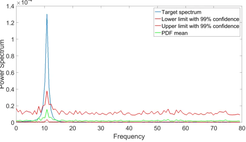
Clearly, the approach developed in the previous section relies on prior knowledge of
164
the correlation between the missing data. Among the various available techniques in the
165
literature for estimating data correlation relationships a Kriging based scheme (e.g. (Stein
166
1999); (Gaspar et al. 2014) and (Jia and Taflanidis 2013)) is considered in the ensuing
167
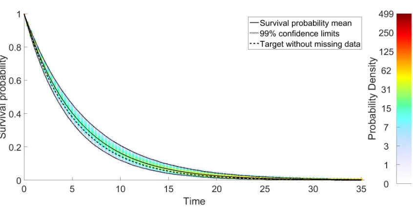
analysis.
168
Specifically, letf(t) be a sample of a stationary stochastic process with a power spectrum
169
Sf(ω). Given the n known pointsti, i= 1,2, ..., n, an estimate off(tj) at the missing point 170
tj, can be obtained as a weighted linear combination of the available known points (Stein
171
1999), i.e.,
172
f(tj) = n X
i=1
λif(ti) +z(t) (17)
173
where λi is the weight of each known point, and z(t) is a stationary Gaussian process with
174
zero mean and covariance
175
C =cov(z(ti), z(ti−tj)) =γ(|ti−tj|) =σz2R(|ti−tj|) (18) 176
where σ2
z is the constant variance of the process and R is the correlation function. Several
177
types of correlation functions, such as exponential, linear and Gaussian, have been proposed
178
in the literature (Kaymaz 2005). Herein, a correlation function of exponential form is adopted
due to its applicability in a wide range of engineering processes (Spanos et al. 2007), i.e.
180
γ(h) = σ2ze−θ1|h|cos(θ
2h)(1 +θ1|h|) (19)
181
where h = ti −tj is the interval between two time instants, and θ1, θ2 are constant values
182
to be determined. Next, σ2
z, θ1 and θ2 are obtained by least-squares fitting of eq.19 to the 183
available data, i.e.,
184
min
σ2
z,θ1,θ2
|γ(h)−γe(h)|2 (20) 185
where| · |2 denotes the L-2 norm, γe(h) = 1nPni=1[f(ti+h)f(ti)], andf(ti+h), f(ti) are the 186
known points.
187
Further, utilizing the Kriging model of Eq.(17) the estimate error variance is given by
188
V =V ar[f∗(tj)−f(tj)] = 2 n X
i=1
λiγ(|ti−tj|)− n X
i=1 n X
k=1
λiλkγ(|ti−tk|)−σz2 (21) 189
Next, to minimize the error variance V, a Lagrange multipliers approach is applied
yield-190
ing the equations
191
Pn
i=1λiγ(|ti−tk|) +κ=γ(|ti−tj|),(j = 1, ..., n) Pn
i=1λi = 1
(22)
192
to be solved for the weights λi and Lagrange multiplier κ . Further, an estimate of the
193
missing point is given by Eq.(17). Then, the covariance matrix C of the sample could be
194
easily obtained through Eq.(18).
195
Note that, denoting the time history vector x as x = (xβ, xα), the covariance matrix C
196
can be expressed as C =
Cββ Cβα
Cαβ Cαα
, where Cββ is the matrix whose rows and columns
197
correspond to the missing pointsxβ, whileCαα corresponds to the known pointsxα. In this
198
regard, the conditional covariance matrix Σ of the missing points is calculated as (Papoulis
and Pillai 2002)
200
Σ =C{xβ|xα}=Cββ−CβαCαα−1Cαβ (23) 201
Overall, adopting a Kriging modeling approach in this section, the mean and covariance of
202
missing data are estimated, and can be used as an input to the approach developed in the
203
previous section.
204
205
Stochastic process spectral moment estimate uncertainty quantification under 206
missing data 207
For stationary random processes, the spectral moments are defined as
208
λi = Z +∞
−∞
ωiS(ω)dω (24)
209
where S(ω) is the two-sided power spectrum (e.g. (Lutes and Sarkani 2004)). Considering
210
next the case of a zero mean process, the zero spectral momentλ0is equal to the mean square
211
E[X2] of the processX (also equal to the squared standard deviation σ2X in this case), and
212
the second spectral moment λ2 is the mean square E[ ˙X2] of the derivative process X.In a
213
similar manner as the moments of a random variable are used to describe certain features
214
of the related PDF, spectral moments are indispensable in a variety of applications such as
215
determining approximately the survival probability (or equivalently, the first-passage time)
216
and assessing the reliability of structural systems (e.g. (Vanmarke 1972); (Vanmarke 1975);
217
(Lutes and Sarkani 2004)).
218
Further, Eq.(24) can be recast into a discrete form in the frequency domain, i.e.
219
λi = X
n
ωinS(ωn)∆ω (25)
220
Clearly, based on Eq.(25) the spectral moment can be viewed as a linear combination
221
of individual power spectrum points. Note that although the PDFs of the power spectrum
points S(ωn) can be obtained by the methodology developed in the previous sections, a 223
straightforward determination of the PDF of the spectral moment λi can be quite daunting
224
due to the following reasons. First, the various power spectrum points S(ωn) do not, in
225
general, follow the same PDF for different frequency valuesωn. Second, the variablesS(ωn) 226
exhibit correlation as they are defined by utilizing the same set of random variables.
227
Next, to address these challenges, a methodology based on characteristic functions is
228
proposed. The characteristic function of a random variable is defined as (Papoulis and Pillai
229
2002)
230
ΦX(ω) = E[eiωx] = Z +∞
−∞
fX(x)eiωxdx (26)
231
where fX(x) is the probability density function of X. Clearly, the characteristic function
232
and the PDF of a random variable form a Fourier transform pair. Further, the spectral
233
moment Eq.(25) can be construed as a quadratic transformation of the missing points Xβ.
234
The correlated variablesXβ ∼N(µ, Σ), whereΣ can be cast into the Cholesky factorization
235
formΣ =AA0 (Abeing a lower triangular matrix), are replaced by a new set of independent
236
standard Gaussian variablesXg ∼N(0,I) as 237
Xβ =µ+AXg (27)
238
Next, employing Eqs.(25-27), Eq.(5) can be cast in the matrix form 239
Sf(ωk) = (c1,k+a0kµ+a 0
kXg)2 + (c2,k+b0kµ+b
0
kXg)2 =Xgn0 BkXgn (28)
240
where c1,k, c2,k,ak, and bk are defined by Eq.(6-9),
241
Xgn = [Xg0,1] 0
= [xg1, xg2, ..., xgu,1]0, (29)
and 243 Bk,ij =
ak,iak,i+bk,ibk,i, i, j ≤u
(c1,k +a0kµ)ak,i+ (c2,k+b0kµ)bk,i, j =u+ 1, i6=u+ 1
(c1,k +a0kµ)ak,j+ (c2,k+b0kµ)bk,j, i=u+ 1, j 6=u+ 1
(c1,k +a0kµ)2+ (c2,k+b0kµ)2, i=j =u+ 1
(30)
244
Combining Eqs.(25) and (29), the spectral moments are given, alternatively, in the form
245
λi =Xgn0
X
k
ωki∆ωBk
!
Xgn (31)
246
whereas utilizing Eq.(31) the characteristic function of the spectral moments becomes
(Pa-247
poulis and Pillai 2002)
248
Φλi(ω) =E[e
iωλi] =
Z +∞
−∞
(2π)−u2 exp −1
2
"
Xg0Xg−iωXgn0 X
k
ωik∆ωBk ! Xgn #! dxg (32) 249
Note that, the evaluation of Eq.(32) can be simplified based on the following steps.
250
Specifically,
251
1) Let
252
Y = 1 2
"
Xg0Xg −iωXgn0 X
k
ωik∆ωBk !
Xgn #
(33)
253
Eq.(33) can be divided into two parts, i.e., Y = Y1 +Y2. The first includes the second
254
order terms, i.e. Y1 =Pi,jcijxgixgj ,while the second includes the first order terms plus the 255
constant term, i.e. Y2 =
P
icixgi+ccons . Thus, Eq.(32) can be rewritten as 256
Φλi(ω) =E[e
iωλi] =
Z +∞
−∞
(2π)−u2e−Y1−Y2dx
g (34)
257
258
2) Similar to Eq.(31),Y1 can be expressed asY1 =Xg0BY1Xg where BY1 is given by
260
BY1 =A
0
Y1AY1 (35)
261
In Eq.(35)AY1 is a complex upper triangular matrix. Here, A
0
Y1 indicates the non-conjugate
262
transpose ofAY1, similarly in Eq.36. The factorization in Eq.(35) is numerically implemented
263
via a Cholesky factorization kind algorithm (Golub and Van Loan 1996) with the note that
264
the diagonal elements in BY1 are complex values.
265
266
3) After obtaining the upper triangular matrix AY1, Y may be expressed in a similar form
267
toY1 (after accounting for first order terms and the constant); thus simplifying the solution
268
of the integral in Eq.(34). Hence
269
Y = (AYXgn)0(AYXgn) +cY (36)
270
where AY = (AY1, au×1), and au×1 are the coefficients to account for the first order terms
271
P
iXgi in Y2 (with u being the number of missing data); and cY is a constant. A worked
272
2-variable example is shown in detail in Appendix.
273
274
4) Finally, substituting Eq.(36) into Eq.(32), the integral in Eq.(32) may be simplified
sig-275
nificantly to a function of BY1, and the constant termcY in the form
276
Φλi(ω) =E[e
iωλi] = 2−u2(det(B
Y1))
−12
e−cY (37)
277
whereas the spectral moments PDFs are estimated via the inverse Fourier transform of
278
Eq.(32), i.e.
279
pλi(s) =
1 2π
Z +∞
−∞
Φλi(ω)e
iωsdω (38) 280
In this section an efficient approach has been developed for quantifying the uncertainty
in the spectral moments estimates of an underlying stochastic process based on available
282
realizations with missing data. Specifically, a closed form expression has been derived in
283
Eq.(32) for the spectral moment characteristic function. The rather daunting brute force
284
numerical evaluation of the integral appearing in the derived expression has been
conve-285
niently circumvented via a Cholesky kind decomposition of the integrand function. Clearly,
286
the development in this section is of considerable importance (as illustrated in the following
287
section) to various engineering dynamics applications such as to structural system reliability
288
assessment (Vanmarke 1975).
289
290
Survival probability estimate uncertainty quantification under missing data 291
A persistent challenge in the field of stochastic dynamics has been the determination
292
of the system survival probability, i.e. the probability that the structural system response
293
will stay below a certain threshold over a given period of time. Many research efforts for
294
addressing the aforementioned challenge exist in the literature ranging from semi-analytical
295
to purely numerical approaches (e.g. (Spanos and Kougioumtzoglou 2014); (Bucher 2001);
296
(Au and Beck 2001)). One of the first semi-analytical approximate approaches proposed by
297
Vanmarke (Vanmarke 1975) that relies on the knowledge of the system response spectral
298
moments (Vanmarke 1972) is considered next.
299
Specifically, consider a linear single-degree-of-freedom (SDOF) oscillator, whose motion
300
is governed by the stochastic differential equation
301
¨
x+ 2ζ0ω0x˙ +ω20x=w(t) (39)
302
where x is the response displacement, a dot over a variable denotes differentiation with
303
respect to time t; ζ0 is the ratio of critical damping; ω0 is the oscillator natural frequency 304
and w(t) represents a Gaussian, zero-mean stationary stochastic process possessing a
broad-305
band power spectrum S(ω). Focusing next on the stationary response of the oscillator, the
response displacement and velocity power spectra are given by (Newland 1993)
307
SX(ω) =|H(ω)|2S(ω) (40)
308
and
309
SX˙(ω) = ω2SX(ω) =ω2|H(ω)|2S(ω) (41) 310
respectively; and the frequency response function H(ω) is given by
311
H(ω) = 1
ω2
0 −ω2+ 2iζ0ω0ω
(42)
312
According to (Vanmarke 1975) and (Crandall 1970), the time-dependent survival proba-313
bility LD(t) of a linear oscillator given a barrier level D can be approximated by
314
LD(t) = exp
"
−1
π
s
λX,2
λX,0
t exp
− D
2
2λX,0
#
(43)
315
whereλX,iis thei-th order spectral moment of the displacementx. Note that for the specific 316
case of the linear oscillator of Eq.(39), and considering a low value for the damping ratio,
317
i.e. ζ0 ≤ 0.05, its response exhibits a narrow-band feature in the frequency domain due to
318
the form of the frequency response function (see Eq.(40)). In particular, it can be seen that
319
|H(ω)|2 is a function with a sharp peak around the oscillator natural frequencyω =ω 0, and 320
decays quickly for ω 6= ω0. Thus, it is reasonable to assume that the response of the linear
321
oscillator exhibits a pseudo-harmonic behavior (Spanos 1978), and the response displacement
322
and velocity can be represented, respectively, as
323
x=acos(ω0t+ϕ) (44)
324
and
325
˙
x=−aω0sin(ω0t+ϕ) (45)
In Eq.(44), a and ϕrepresent the response amplitude and phase processes, respectively; see
327
also (Spanos 1978) and (Kougioumtzoglou and Spanos 2012) for more details. Considering
328
next Eqs.(44-45), the independence of a with ϕ and taking into account thatE(cos2(ω
0t+ 329
ϕ)) =E(sin2(ω0t+ϕ)) yields 330
E( ˙x2) =ω02E(x2) (46)
331
or in other words
332
λX,2 =ω02λX,0 (47)
333
Substituting Eq.(47) into Eq.(43) yields an approximate expression for the oscillator survival
334
probability that depends only on λX,0, i.e. 335
LD(t) = exp
−ω0
π t exp
− D
2
2λX,0
(48)
336
In Eq.(48), the analytical expression for the PDF of λX,0 in the case of missing data can
337
be derived by the methodology described in the previous sections. After determining the
338
PDF pλX,0 , the system survival probability characteristic function can be obtained as
339
ΦLD(ωk) =E[e
iωkLD] =
Z +∞
−∞
eiωkLDp
λX,0dλX,0 (49)
340
whereas, an inverse Fourier transform can applied to Eq.(49) for numerically evaluating the
341
survival probability PDF.
342
343
NUMERICAL EXAMPLES 344
Excitation records with missing data 345
To demonstrate the validity of the developed uncertainty quantification approach,
sta-346
tionary stochastic process time histories compatible with the Kanai-Tajimi-like earthquake
engineering power spectrum of the form
348
S(ω) = S0
ω4
g + 4ζg2ωg2ω2
(ω2
g −ω2)2+ 4ζg2ω2gω2
(50)
349
where ωg = 5πrad/s and ζg = 0.63 , are generated via Eq.(2) with a time duration of
350
8.64 seconds and time step of 0.039 seconds. To compare with the method described in
351
(Comerford et al. 2015b), a factor S0 = 0.011 is introduced to make the standard deviation
352
equal to 1. Next, uniformly randomly distributed missing data are artificially induced to
353
provide a Monte-Carlo simulation comparison; 10,000 samples are used in the following 354
results.
355
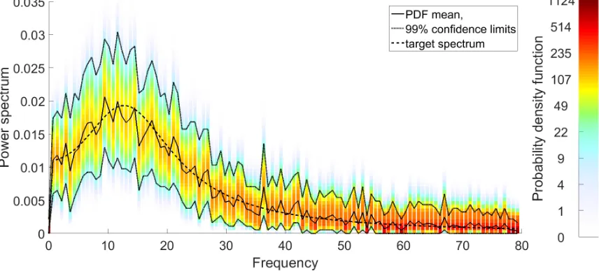
Figure 1 shows the estimated power spectrum PDFs and confidence ranges determined
356
via the herein developed approach for 10% missing data. For comparison purposes Figure
357
2 is the result of applying the methodology in (Comerford et al. 2015b), where
correla-358
tions between missing data are not taken into consideration and the missing points follow
359
independent identical Gaussian distributions Xβ ∼ N(0,I). Compared with Figure 2, the
360
method developed herein provides with a smaller range, and the mean spectrum fits the
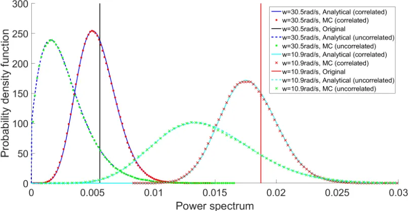
orig-361
inal spectrum better. Figure 3 shows the PDFs corresponding to frequencies 10.9 and 30.5
362
rad/s with 10% missing data replaced both by correlated and by independent identically
363
distributed Gaussian random variables. The vertical lines correspond to the spectral values
364
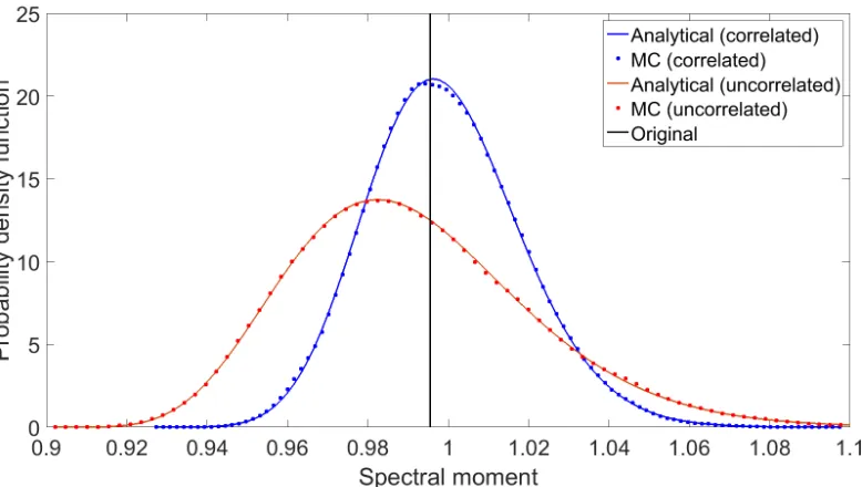
without missing data. Figure 4 shows the spectral moment λ0 of the excitation spectrum,
365
compared with pertinent Monte Carlo simulations. It can be readily seen that in all cases
366
accounting for the correlation of the missing data, as estimated via the Kriging model, yields
367
spectral estimates PDFs that are much closer to the true value.
368
369
Structural response records with missing data 371
In the second example, consider a linear oscillator with ω0 = 10.9rad/s, and ζ0 = 0.05. 372
Further, the missing data are introduced into the stationary records of the oscillator response,
373
which are generated by utilizing the same excitation spectrum as in the first example, and
374
by numerically solving the equation of motion. Similarly, the artificially induced missing
375
data in the response records are uniformly randomly distributed, this time with 100,000
376
Monte-Carlo samples utilized for increased accuracy in the spectral moment comparison.
377
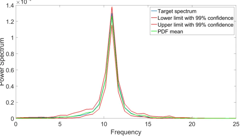
Figure 5 shows the power spectrum PDF and confidence ranges of the oscillator response
378
with 70% missing data determined by the herein developed methodology. For comparison
379
purposes Figure 6 is the result of applying the methodology in (Comerford et al. 2015b),
380
where correlations between missing data are not taken into consideration and the missing
381
points follow independent identical Gaussian distributions. As anticipated, it can be readily
382
seen that neglecting the correlation structure in the missing data has a bigger negative effect
383
when considering narrow-band signals(see Figures 5 and 6) rather than broad-band ones (see
384
Figures 1 and 2). In fact, for the highly correlated oscillator response process disregarding
385
the correlation structure yields an almost constant power spectrum estimate value. Figure 7
386
shows the PDF of the response spectral moment λ0, compared with pertinent Monte Carlo
387
simulations. In Figure 8 the PDF of the oscillator survival probability Eq.(48) with 70%
388
missing data and a barrier level a = 0.05 is plotted and compared with pertinent Monte
389
Carlo simulations of Eq.(43).
390
391
CONCLUSION 392
In this paper, an analytical approach for quantifying the uncertainty in stochastic
pro-393
cess power spectrum estimates based on samples with missing data has been developed.
394
Specifically, the correlations between the missing data are considered by employing a
Krig-395
ing model, while utilizing fundamental concepts from probability theory, and resorting to a
396
Fourier based representation of stationary stochastic processes, a closed form expression has
been derived for the power spectrum estimate PDF at each frequency. Next, the approach
398
has been extended for determining the PDF of spectral moments estimates as well. This is
399
of considerable significance to reliability assessment methodologies as well, where spectral
400
moments are used for evaluating the survival probability of the system. Further, it has been
401
shown that utilizing a Cholesky kind decomposition for the PDF related integrals the
com-402
putational cost is kept at a minimal level. Several numerical examples have been presented
403
and compared against pertinent Monte Carlo simulations for demonstrating the validity of
404 the approach. 405 406 ACKNOWLEDGEMENTS 407
The first author is grateful for the financial support from the China Scholarship Council.
408
409
APPENDIX 410
By factorizing part of the integrand of Eq.(32) (given as Y in Eq.(33), the solution of
411
Eq.(32) may be greatly simplified. In the following, a 2-variable case is given as an example.
412
For a 2-variable case, Eq. (31) becomes
413
λi =ax21+bx1x2+cx22+dx1+ex2+f (51) 414
wherea, b, c, d, e, f are real constant witha >0, c > 0, f >0. Eq.(51) can be also recast into
415
a matrix form as
416
λi =
x1 x2 1
a 0.5b 0.5d
0.5b c 0.5e
0.5d 0.5e f
x1 x2 1 (52) 417
Further, according to Eq.(33), Y has the form
418
Y = 1 2x 2 1+ 1 2x 2
The object of step 3 is to recast Eq.(53) into the form given by Eq.(36). To achieve this
420
goal, second order terms of Y are separated and then factorized as follows,
421
Y1 =
1 2x 2 1+ 1 2x 2
2−iω(ax 2
1+bx1x2+cx22)
=
x1 x2
0.5−iωa −0.5iωb
−0.5iωb 0.5−iωc
x1 x2 =
x1 x2
A0Y1AY1
x1 x2 (54) 422
where AY1 =
√
0.5−iωa − iωb
2√0.5−iωa
0
r
ω2b2
2−4iωa + 0.5−iωc
, and A
0
Y1 is the non-conjugate
trans-423
pose of AY1, i.e., A
0
Y1AY1 =
0.5−iωa −0.5iωb
−0.5iωb 0.5−iωc
. This calculation can use follow the
424
same numerical implementation steps as a Cholesky factorization algorithm with the note
425
that
0.5−iωa −0.5iωb
−0.5iωb 0.5−iωc
is not a Hermitian positive-definite matrix. Then, extending
426
Y1 to account for the first order terms in Eq.(53), Y may be written as,
427
Y = 1 2x 2 1+ 1 2x 2
2−iω(ax 2
1+bx1x2 +cx22+dx1+ex2+f)
=
x1 x2
A0Y1AY1
x1 x2
−iω(dx1+ex2+f)
= (AY x1 x2 1
)0(AY x1 x2 1
) +cY
(55)
whereAY = √
0.5−iωa − iωb
2√0.5−iωa − iωd 2√0.5−iωa
0
r
ω2b2
2−4iωa + 0.5−iωc
bdω2
1−2iωa−iωe
2
v u u t
ω2b2
2−4iωa+0.5−iωc
0 0 0
,cY =−(−2√0.5iωd−iωa)2− 429
(
bdω2
1−2iωa−iωe
2
v u u t
ω2b2
2−4iωa+0.5−iωc
)2−iωf. 430
Calculating the first term in Eq.(55), it can be seen that (AY
x1 x2 1
)0(AY x1 x2 1 ) takes 431 the form 432
(AY x1 x2 1
)0(AY x1 x2 1
) = (m1x1+m2x2+m3)2+ (m4x2+m5)2 (56) 433
where the constants m1, m2, m3, m4, m5 are calculated by AY. Hence, Y may be written as 434
Y = (m1x1+m2x2 +m3)2 + (m4x2 +m5)2 +cY (57) 435
The form Eq.(57) is particularly useful in calculating the integral in Eq.(32), allowing it
436
to be simplified as shown
437
Φλi(ω) = E[e
iωλi] =
Z +∞
−∞
(2π)−u2exp(−Y)dxg
= (2π)−1
Z Z +∞
−∞
exp[−(m1x1+m2x2+m3)2−(m4x2+m5)2−cY]dx1dx2
= (2π)−1
√
π m1
Z +∞
−∞
exp[−(m4x2+m5)2−cY]dx2
= 1
2m1m4
exp(−cY)
(58)
438
For the general multi-variable case, the above steps are the same.
439
Au, S.-K. and Beck, J. (2001). “Estimation of small failure probabilities in high dimensions
441
by subset simulation.” Prob. Eng. Mech., 16(4), 263–275.
442
Billingsley, P. (2008). Probability and measure. John Wiley & Sons.
443
Bucher, C. (2001). “Simulation methods in structural reliability.” Marine Technology and
444
Engineering, 2, 1071–1086.
445
Comerford, L., Jensen, H., Mayorga, F., Beer, M., and Kougioumtzoglou, I. (2017).
“Com-446
pressive sensing with an adaptive wavelet basis for structural system response and
relia-447
bility analysis under missing data.”Computers & Structures, 182, 26–40.
448
Comerford, L., Kougioumtzoglou, I. A., and Beer, M. (2014). “Compressive sensing based
449
power spectrum estimation from incomplete records by utilizing an adaptive basis.”
Pro-450
ceedings of IEEE SSCI 2014, 117–124. doi:10.1109/CIES.2014.7011840.
451
Comerford, L., Kougioumtzoglou, I. A., and Beer, M. (2015a). “An artificial neural
net-452
work approach for stochastic process power spectrum estimation subject to missing data.”
453
Structural Safety, 52, 150–160.
454
Comerford, L., Kougioumtzoglou, I. A., and Beer, M. (2015b). “On quantifying the
uncer-455
tainty of stochastic process power spectrum estimates subject to missing data.”
Interna-456
tional Journal of Sustainable Materials and Structural Systems, 2(1-2), 185–206.
457
Comerford, L., Kougioumtzoglou, I. A., and Beer, M. (2016). “Compressive sensing based
458
stochastic process power spectrum estimation subject to missing data.”Probabilistic
En-459
gineering Mechanics. doi:10.1016/j.probengmech.2015.09.015.
460
Cramer, H. and Leadbetter, R. (1967). Stationary and related stochastic processes: sample
461
function properties and their applications. Wiley.
462
Crandall, S. H. (1970). “First-crossing probabilities of the linear oscillator.”Journal of Sound 463
Vibration, 12(3), 285.
464
Eldar, Y. and Kutyniok, G. (2012). Compressed Sensing: Theory and Apps. Cambridge Uni
465
Press.
466
Gaspar, B., Teixeira, A. P., and Guedes, S. C. (2014). “Assessment of the efficiency of kriging
surrogate models for structural reliability analysis.” Probabilistic Engineering Mechanics,
468
37, 24–34.
469
Golub, G. H. and Van Loan, C. F. (1996).Matrix Computations. Johns Hopkins, Baltimore.
470
Jia, G. and Taflanidis, A. (2013). “Kriging metamodeling for approximation of
high-471
dimensional wave and surge responses in real-time storm/hurricane risk assessment.”
Com-472
puter Methods in Applied Mechanics and Engineering, 261-262, 24–38.
473
Kaymaz, I. (2005). “Application of kriging method to structural reliability problems.”Struct.
474
Saf., 27(2), 133–151.
475
Kougioumtzoglou, I. A., dos Santos, K. R., and Comerford, L. (2017). “Incomplete data
476
based parameter identification of nonlinear and time-variant oscillators with fractional
477
derivative elements.”Mechanical Systems and Signal Processing, 94, 279 – 296.
478
Kougioumtzoglou, I. A., Kong, F., Spanos, P. D., and Li, J. (2012). “Some observations
479
on wavelets based evolutionary power spectrum estimation.”Proceedings of the Stochastic
480
Mechanics Conference (SM12), 37–44. ISSN: 2035-679X.
481
Kougioumtzoglou, I. A. and Spanos, P. D. (2012). “An analytical wiener path integral
tech-482
nique for non-stationary response determination of nonlinear oscillators.” Probabilistic
483
Engineering Mechanics, 22, 125–131.
484
Lutes, L. D. and Sarkani, S. (2004).Random vibrations: analysis of structural and mechanical
485
systems. Elsevier.
486
Newland, D. E. (1993). An introduction to random vibrations, spectral and wavelet analysis.
487
Dover Publications.
488
Papoulis, A. and Pillai, S. U. (2002).Probability, Random Variables and Stochastic Processes.
489
McGraw-Hill.
490
Politis, N. P., Giaralis, A., and Spanos, P. D. (2007). “Joint time-frequency representation
491
of simulated earthquake accelerograms via the adaptive chirplet transform.” Proc.
Com-492
putational stochastic Mechanics, 549–557.
493
Priestley, B. (1982). Spectral analysis and time series. Academic Press.
Qian, S. (2002). Introduction to Time-Frequency and Wavelet Transforms. Prentice Hall.
495
Shinozuka, M. and Deodatis, G. (1991). “Simulation of stochastic processes by spectral
496
representation.”Appl. Mech. Rev., 44(4), 192–203.
497
Spanos, P. D. (1978). “Non-stationary random vibration of a linear structure.”International
498
Journal of Solids and Structures, 14, 861–867.
499
Spanos, P. D., Beer, M., and Red-Horse, J. (2007). “Karhunen–lo`eve expansion of stochastic
500
processes with a modified exponential covariance kernel.”Journal of Engineering
Mechan-501
ics, 133(7), 773–779.
502
Spanos, P. D. and Failla, G. (2004). “Evolutionary spectra estimation using wavelets.” J.
503
Eng. Mech., 130, 952–960.
504
Spanos, P. D. and Kougioumtzoglou, I. A. (2014). “Survival probability determination of
505
nonlinear oscillators subject to evolutionary stochastic excitation.” Journal of Applied
506
Mechanics, 81, 051016–1 051016–9.
507
Stein, M. (1999). Interpolation of Spatial Data: Some Theory for Kriging. Springer-Verlag,
508
New York.
509
Vanmarke, E. H. (1972). “Properties of spectral moments with applications to random
vi-510
bration.” Journal of Engineering Mechanics Division, 98, 425.
511
Vanmarke, E. H. (1975). “On the distribution of the first passage time for normal stationary
512
random process.” Journal of Applied Mechanics, 215–220.
513
Wang, Y., Li, J., and Stoica, P. (2005). Spectral Analysis of Signals, the Mising Data Case.
514
Morgan & Caypool.
List of Figures 516
1 Power spectrum probability densities with 10% missing data replaced by
cor-517
related Gaussian random variables . . . 26
518
2 Power spectrum probability densities with 10% missing data replaced by
in-519
dependent identically distributed Gaussian random variables . . . 27
520
3 PDFs at 10.9 and 30.5 rad/s with 10% missing data replaced by both
cor-521
related and independent identically distributed Gaussian random variables.
522
Monte-Carlo estimated PDFs (MC) are shown for validation of the
proce-523
dure. The vertical line shows the spectral value without missing data . . . . 28
524
4 PDF of spectral momentλ0 with 10% missing data replaced by both correlated
525
and independent identically distributed Gaussian random variables.
Monte-526
Carlo estimated PDFs (MC) are shown for validation of the procedure. The
527
vertical line shows the spectral moment λ0 value without missing data . . . . 29
528
5 Oscillator response power spectrum PDF with 70% missing data replaced by
529
correlated Gaussian random variables . . . 30
530
6 Oscillator response power spectrum PDF with 70% missing data replaced by
531
independent identically distributed Gaussian random variables . . . 31
532
7 PDF of response spectral moment λ0 with 70% missing data. The
Monte-533
Carlo estimated PDF (MC) is shown for validation of the procedure. The
534
vertical line shows the spectral moment without missing data . . . 32
535
8 Survival probability of oscillator response with 70% missing data and barrier
536
a= 0.05 via Eq.(48); comparisons with pertinent Monte Carlo simulations of
537
Eq.(43) . . . 33
FIG. 8. Survival probability of oscillator response with 70% missing data and barrier