Invariants of toric seiberg duality

City, University of London Institutional Repository

Citation

:

This is the accepted version of the paper.

This version of the publication may differ from the final published

version.

Permanent repository link:

Link to published version

:

Copyright and reuse:

City Research Online aims to make research

outputs of City, University of London available to a wider audience.

Copyright and Moral Rights remain with the author(s) and/or copyright

holders. URLs from City Research Online may be freely distributed and

linked to.

IMPERIAL/TP/11/AH/06 QMUL-PH-11-05

Invariants of Toric Seiberg Duality

Amihay Hanany

_{Yang-Hui He}

_{Vishnu Jejjala}

_{Jurgis Pasukonis}

Sanjaye Ramgoolam

_{and Diego Rodriguez-Gomez}

1 _{Theoretical Physics Group, The Blackett Laboratory,}

Imperial College, Prince Consort Road, London SW7 2AZ, UK

2 _{Department of Mathematics, City University, London,}

Northampton Square, London EC1V 0HB, UK;

School of Physics, NanKai University, Tianjin, 300071, P.R. China; Merton College, University of Oxford, OX14JD, UK

3 _{Department of Physics, Queen Mary, University of London,}

Mile End Road, London E1 4NS, UK

4 _{Department of Physics, Technion, Haifa, 3200, Israel;}

Department of Mathematics and Physics, University of Haifa at Oranim, Tivon, 36006, Israel

Abstract

Three-branes at a given toric Calabi–Yau singularity lead to different phases of the con-formal field theory related by toric (Seiberg) duality. Using the dimer model/brane tiling description in terms of bipartite graphs on a torus, we find a new invariant under Seiberg duality, namely the Kleinj-invariant of the complex structure parameter in the distinguished isoradial embedding of the dimer, determined by the physicalR-charges. Additional number theoretic invariants are described in terms of the algebraic number field of the R-charges. We also give a new compact description of the a-maximization procedure by introducing a generalized incidence matrix.

∗ _{a.hanany@imperial.ac.uk, yang-hui.he.1@city.ac.uk, v.jejjala@qmul.ac.uk, j.pasukonis@qmul.ac.uk,}

s.ramgoolam@qmul.ac.uk, drodrigu@physics.technion.ac.il

Contents

1 Introduction 3

2 Dimer models and Seiberg duality 4

2.1 a-maximization for dimer models . . . 6

2.2 Seiberg duality and the invariance ofτR. . . 8

3 A proof of j(τR) as a Seiberg duality invariant 10 3.1 A closer look at urban renewal . . . 10

3.1.1 Integrating out massive fields . . . 14

3.1.2 Physics of the assumption of local rigidity . . . 16

3.2 j(τR) is an invariant under Seiberg duality . . . 18

4 τR from toric data 18 4.1 a-maximization from toric diagram . . . 19

4.2 Explicit τR and two-dimensional a-maximization . . . 21

5 a-maximization and invariants in terms of generalized incidence matrix 23 5.1 Lagrange multipliers and a-maximization . . . 23

5.2 Properties of the generalized incidence matrix . . . 27

5.3 Applications: _C3 _{and SPP . . . . 29}

6 Number theoretic invariants of Seiberg duality 31 7 Concluding remarks and open questions 34 A Examples of τR 36 A.1 _C3 _{. . . . 36}

A.2 SPP . . . 37

1

Introduction

Thanks to the seminal work of N. Seiberg, strong coupling/weak coupling duality in non-Abelian N = 1 super-Yang–Mills (SYM) theories is well-established [1].1 This duality has been used and tested extensively in various environments, and it is now part of the standard toolkit of the (supersymmetric) field theorist.

Seiberg duality is a purely field theoretic statement. Nevertheless, it is often interesting to examine it from a string theoretic perspective. A “proof” of the duality may be established by means of operations in a brane configuration [2]. In this paper we will mostly be interested in gauge theories arising from D3-branes probing a toric Calabi–Yau threefold (CY3) singularity.

As first noted in [3–6], within this context Seiberg duality is the field theory manifestation of toric duality, wherein, different, but equivalent, descriptions of the same CY3 are related

by Seiberg duality of the associated field theories. By now a heavy mathematical technology has been developed to understand the class of theories under discussion in which different nuances of Seiberg duality have been appreciated (see e.g., [7–15]).

D3-branes probing conical CY3 geometries are of special interest, as they give rise to

examples of the AdS5/CFT4 correspondence [16–18] with N = 1 supersymmetry. These

dualities have been particularly studied when the CY3 is toric. In fact, infinite series of

explicit examples where both metric and field theory are known have been presented in [19– 22]. Further progress was made in [23] where it was shown that these field theories — which flow to non-trivial IR superconformal fixed points — dual to D3-branes probing toric CY3

geometries, can be neatly encoded in a bipartite graph drawn on a torus; this graph is called a dimer [24] or brane tiling [23]. In [25], it was shown how the dimer is related, through mirror symmetry, to a system of intersecting D6-branes. This mirror Type IIA configuration is as well related by T-duality to a five brane system from which the dimer can be read. We refer to [26, 27] for thorough reviews.

A further refinement on the dimer was introduced in [28], where it was shown how the

R-charges can be encoded in certain angles in the dimer once it is drawn in a particu-lar, isoradial manner. In fact, isoradial embeddings for dimers have been introduced in the mathematical literature (for a review see e.g., [29]). When the angles in the isoradial dimer are associated to the physical R-charges (which maximize the trial R-charges in the

a-maximization procedure), a distinguished complex structure (shape) of the torus is deter-mined. This complex structure is denoted as τR and has been studied in [30, 31].

In [30], it was noted that the mathematical theory of dessins d’enfants enables us to 1 _{We should note that no strict proof has been given for generic cases. Nevertheless, there is virtually no}

uniquely express bipartite graphs on a Riemann surface Σ equivalently in terms of a holo-morphic map β : Σ →_P1 _{with three branch points that can be chosen to lie at {0,1,∞}.}

The pull-back of the unique complex structure of the_P1 _{to Σ determines a complex structure}

on Σ. For the case of a dimer drawn on a torus _T2_{, we have a complex structure τ}

B on an elliptic curve. In infinite families of examples, τB =τR up toSL(2,Z) equivalence, although

we now know that the equality does not always hold [31].2

In this note we study Seiberg duality from the dimer model perspective, where it goes under the name “urban renewal” [23, 32]. Remarkably, the distinguished isoradial torus is the same for each of the different phases of a theory related by Seiberg duality. That is to say, we can think of τR — or more precisely the associated j-invariant j(τR) — as an invariant under Seiberg duality. In this note we will prove this by means of field theoretic methods. It is natural to suspect, however, that this has a more profound geometrical meaning when regarded from a string theoretic perspective. We will postpone this discussion to a forth-coming publication [33]. Furthermore, motivated by the invariance of j(τR) among different Seiberg dual phases, we will introduce a new elegant repackaging of thea-maximization pro-cedure [34] for brane tilings [35, 36]. This is done in terms of a generalized incidence matrix, which also gives a neat expression for further invariants under Seiberg duality.

The paper is structured as follows. Section 2, following a lightning review of dimer model technology for four-dimensional SCFTs, introduces the distinguished isoradial torus and its complex structure τR. By computing a large number of examples, we will motivate that

τR, or more precisely j(τR), is an invariant under Seiberg duality. Section 3 provides a field theoretic proof of this statement. Section 4 revisits τR from direct examination of the toric diagram. Section 5 gives a new description of the a-maximization of dimer models in terms of a generalized incidence matrix. Section 6 considers further invariants of Seiberg duality. Section 7 concludes.

2

Dimer models and Seiberg duality

Dimer models were introduced in [23–25] as an extremely efficient way of packaging field theories arising from D3-branes at the tip of toric CY3 cones over a five-dimensional Sasaki–

Einstein base B. These theories flow in the IR to non-trivial SCFTs, which, by standard decoupling limit arguments [16–18], are dual to Type IIB supergravity on AdS5 × B. We

2 _{Phase two of L}2,2,2 _{supplies a counterexample. Nevertheless, there are many examples for which the}

equality does hold and it would be interesting to investigate how generic this situation is. In fact, the counterexample found in [31] applies to the non-minimal phase ofL2,2,2 obtained by Seiberg dualizing the non-chiral Douglas–Moore orbifold of the conifold, which does satisfy τB =τR. Thus, one might speculate

refer the reader to [27] for an extensive review on the subject.

Briefly, the dimer is a bipartite graph, consisting of black and white nodes, drawn on a torus, _T2_{. The edges of the dimer correspond to the fields of the SCFT and, by the}

bipartite condition, connect nodes of opposite color. The nodes themselves encode the superpotential W: black nodes correspond to monomial traces in W with a −1 coefficient, while white nodes correspond to monomials of coefficient +1. The monomials are then reconstructed by arranging the fields as an ordered string choosing, say, counterclockwise orientation for black nodes and clockwise for white nodes. Finally, edges enclose faces, which in turn correspond to gauge groups of equal rank: an edge separating face ifrom face

j corresponds to a bifundamental field of the gauge groups i and j, with the assignment of fundamental gauge groupiand antifundamental gauge groupjdetermined by the orientation of the embedding torus. Such a graph can be thought of as dual to a periodic version of the familiar quiver diagram representation of the gauge theory. The dimer model can be interpreted as a tiling [21, 28], by NS-branes and D-branes, serving as a generalization of brane box models [37, 38]. We illustrate the dimer with the canonical example of N = 4 super-Yang–Mills theory, which corresponds to the trivial toric non-compact Calabi–Yau threefold _C3 _{in Figure 1.}

As mentioned above, the field theories under investigation flow to a non-trivial IR fixed point. At the fixed point there is a particular U(1)R that is part of the supermultiplet that contains the stress-energy tensor. Thus the charges under this U(1), viz., the R-charges, of chiral operators X are identified with their scaling dimensions as ∆[X] = 3₂R[X]. In principle, this superconformal R-charge is an unknown non-anomalous combination of all the globalU(1) symmetries of the theory. A priori, accidental U(1) symmetries may appear along the flow to the IR and mix with the superconformal R-symmetry, so one might worry that the latter is not visible in the UV theory. However, it is known this is not the case, as potential accidental Abelian symmetries, which have been shown to appear only for theories dual to geometries with four-cycles [39], are spontaneously broken along the flow and hence do not mix with the fixed point R-symmetry. Thus, the IR R-symmetry for the theories of interest is in fact a combination of the non-anomalous Abelian symmetries visible in the UV Lagrangian. As a further check, the non-anomalous orthogonal Abelian symmetries become baryonic symmetries in the IR fixed point, and it is known (e.g., [23, 40]) that the number of such symmetries matches that expected from the gravity dual, hence supporting the assumption that the IR R-symmetry is already visible in the UV Lagrangian.

As the IR superconformal R-symmetry is visible in the UV, we can thus identify it using the standard a-maximization algorithm3 and trace it back to UV. This provides a natural

3 _{In fact, that no accidental U(1)s mixing with theU(1)}

R appear along the flow is implicitly assumed

choice of R-symmetry, and indeed we will loosely refer to the R-charge of a field as the R -charge under this particularly interestingR-symmetry. It is now expedient to briefly review

a-maximization specialized to the case of the dimer models.

2.1

a

-maximization for dimer models

In this subsection, let us review thea-maximization procedure of [34] when implemented for our dimer models. For conformality we need to impose the vanishing of β-functions, both for gauge coupling and superpotential couplings. First of all, we recall that the NSVZ exact

β-function for the A-th gauge group factor with coupling gA, in terms of the R-charges Ri of all fieldsXi charged underA, is

βA=

3N

2(1− g2AN

8π2 )

"

2− X

i:i∈∂F

(1−Ri)

#

. (2.1)

The sum runs over the sides which bound a face F, indicated by i ∈∂F, since faces corre-spond to gauge groups in the dimer and the edges bounding correcorre-spond to fields transforming under that group. Note that the same field can provide two edges for a single face; this hap-pens when the field transforms under the adjoint representation of the corresponding gauge group. Therefore, the imposition of the vanishing ofβAfor eachArequires that in the dimer, for each face,

X

i:i∈∂F

(1−Ri) = 2 . (2.2)

The condition that the superpotential has R-charge two (or analogously the vanishing of the superpotential coupling β-function) gives the condition that, for each node V in the dimer — which corresponds to a monomial term in the superpotential,

X

i:V∈∂(i)

Ri = 2 . (2.3)

The sum is over edges incident on the vertex V, denoted as V ∈∂(i).

Then, following [34], subject to these constraints of the conformal manifold, one maxi-mizes the triala-functiona:= ₃₂3 (3TrR3_{−TrR) for a set of trialR-charges, where the trace}

indicates a sum over R charges of the fermions (which are one less than that of the bosons in the same multiplet). For our theories, TrR = 0, so we need only maximize

a({Ri}) = d

X

i=1

(Ri−1)3 , (2.4)

Remarkably, the R-charge can be very easily encoded in the dimer. As described in [28], it is particularly convenient to draw the dimer in anisoradial embedding, a concept in fact noted in the mathematical literature (e.g., [29]). The isoradial dimer is such that all nodes lie on the circumference of a circle of unit radius centered upon each face; whence the name isoradial. In fact, there is a moduli space of isoradial embeddings that satisfy this condition. Among these, a particular one, the R-dimer, is selected by the R-charges of the fields in the corresponding N = 1 quantum field theory. As shown in [28], the R-charges of a given bifundamental field Xij, on the interface between facesi and j, can be encoded in the angle

θ subtended between the edge itself and the radius of the circle centered on face iextending to the node where theXij edge starts. Indeed, because of the isoradial condition, this is the same had we chosen the circle centering facej. Thus, the dimer model here is a collection of rhombi. In summary, we have an immediate geometrical formula to read off the R-charge:

θ= π

2R[Xij] . (2.5)

We demonstrate the relevant quantities for our standard example of _C3 _{in Figure 1.}

X θ

Figure 1: The dimer for the N = 4 super-Yang–Mills theory corresponding to the trivial CY3 toric

coneC3. The fundamental region, containing a single pair of white/black nodes — signifying that there is only a single gauge group factor — is marked by the parallelogram in red. The nodes are trivalent,

corresponding to two cubic monomials in the superpotential: W = Tr (XY Z−XZY). We have marked one edge as the fieldX, and the angleθ, in a isoradial embedding — marked by the dotted unit circles — is related to itsR-charge as θ= π₂R(X).

As we have reviewed, the dimer encodes all the relevant information about the field the-ory: the matter content, the gauge sector, and the superpotential can all be read off from the dimer. At this level, the precise _T2 _{on which the dimer is drawn is largely irrelevant.}

Crucially, the isoradial prescription, which allows us to encode the details of the IR super-conformal fixed point asR-charges corresponding to angles, chooses a particular _T2 _{for each}

gauge theory; namely the _T2 _{on which the isoradial dimer fits.}

Since this _T2 _{is fixed, it is natural to consider its properties, in particular its complex}

structure which we will denote asτR. In fact, following the isoradial prescription, and making use of the standard a-maximization tools, it is possible to draw the unit cell of the isoradial dimer from which τR is easily read off. This process can be automated with the help of a computer. Of course, since for any torus, the complex structure is defined only up to modular transformation, we must bear in mind that any SL(2,_Z) action on τR gives the same underlying _T2 _{of the dimer. This quantity τ}

R will turn out to be a distinguishing property of our gauge theories.

2.2

Seiberg duality and the invariance of

τ

We now arrive at the chief topic of our interest, Seiberg duality. Its implementation on the field theory is well known, and we refer to [41] as the classic review. In turn, as described in [23], Seiberg duality can be implemented in the dimer model in a very neat way, in terms of a move in the graph known as urban renewal [23, 32]. Rather than providing a cumbersome description in words, we provide the graphical effect of urban renewal in Figure 2. We note that this move, at least as a graph move, is local in that it only alters the edges (i.e., fields) surrounding the face (i.e., gauge group) undergoing the Seiberg duality. The face undergoing urban renewal is four sided, which in the field theory corresponds to a gauge group with Nf = 2Nc so that both electric and magnetic theories contain SU(Nc) gauge groups.4

That two Seiberg (toric) dual pairs of gauge theories have their corresponding dimer models related by this urban renewal move is well known [23]. In conjunction with our distinguished isoradial embedding, we now come to the principal observation of this paper, namely that different Seiberg dual theories are encoded on dimers which live on the same isoradial dimer. In other words, different Seiberg dual phases of a given theory have the same τR up to an SL(2,Z) transformation. More succinctly, since the Klein j-function is a modular invariant, we can phrase our observation as:

4 _{Of course, it is possible to dualize gauge groups which are not four sided. This will not change the}

R1

R2

R3 R4

U12

U23 U34

U41

S1 S2 S3 S4

U12

U23 U34

U41

T12

T23 T34

T41

Figure 2: Seiberg duality in dimer models implemented by a so called urban renewal, together with appropriate R-charge assignments. With the assumption of rigid local refinement the four nodes on the corners of the dotted rectangle (R-box) remain fixed and only the position of the four new nodes (S-box) are to be determined.

Different Seiberg dual phases of a gauge theory have the same j(τR).

We will prove this statement in the following section. For now, let us give ample support, which we have obtained from experimentation. We turn to the database of dimer models compiled in [42]. Therein, we have many collections of Seiberg dual phases, including perhaps the most famous pair of the theory corresponding to the zeroth Hirzebruch surface _F0 '

P1×P1. We draw the isoradial embedding of all the associated dimer models and compute

theirτR; the results are tabulated in Table 1. The leftmost column denotes the CY3geometry

which the D3-brane probes (dP denotes cones over the del Pezzo surfaces and P dP, the pseudo del Pezzo ones), for bookkeeping, we record the actual τR values of the isoradial embedding of the various phases in the middle column, and the final column is reserved for thej-invariant.5 _{In Table 1, we see that while in some cases, theτ}

R appear to be remarkably different, they share the same value of thej-function, and are thus modular equivalent.

The cases where j(τR) = 0 andj(τR) = 1728 correspond to elliptic curves with enhanced symmetries, _Z2 ×Z3 and Z4, respectively, whereas for a generic value of j(τR), the elliptic curvey2 _{=x(x−1)(x−λ) only enjoys a}

Z2 symmetry corresponding to the invariance under y7→ −y.

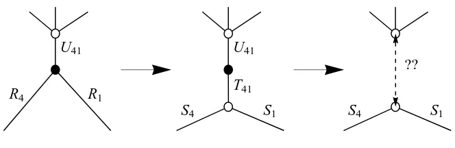
CY3 geometry τR 1728−1j(τR)

F0 i,1 +i 1

L2,2,2 1

5 + 2 5i ,

1 5 +

2

5i '166.375

L2,3,2 _{1 +} 1+√3−1e23i

√

7π

1+5e13i(2+

√

7)π ,

2e12i

√

7π

1+e−13i(

√

7−7)π

cos₍1₆₍2+√7₎π₎

1+5(−1)2/3_e13i

√

7π ' −7489.12

L2,4,2 −3+e−

iπ √ 3 cos π √ 3

−3 , i

i+ 2 tan π

2√3

+ cot π

2√3

746401

L3,3,3 i

3 ,1 +

i

3 '88862.08

dP2

−(−1)9/16e−

1 16i

√

33π₊√4_−1e1₄i√33π_−e21i√33π₊₍₋₁₎15/16_e169i√33π

i−2√4−1e14i

√

33π_+e1₂i√33π ,

16√₋₁

4 √

−1−e14i

√

33π2

(−1)9/16₊₍₋₁₎5/8_e−1

16i

√

33π₋₍₋₁₎5/16_e1₄i√33π_−e169i√33π

'0.169478

dP3 eπi/3 , eπi/3 , eπi/3 , eπi/3 0

P dP3b 1 +icos

√ 5π 2 csc

3√5π

2

,1 +icos

√ 5π 2 csc

3√5π

2

'1.02155

Table 1: The values ofτRfor different Seiberg dual faces of a theory are SL(2,Z) equivalent.

3

A proof of

j

(

τ

)

as a Seiberg duality invariant

We now present a proof of the claim in the previous section. To that end, we need to develop a finer understanding of the Seiberg duality procedure implemented on the dimer as an urban renewal move. As usual, we will adhere to the terminology that the theory before Seiberg duality/urban renewal, is electric and the one after is magnetic.

3.1

A closer look at urban renewal

As a graph theoretic operation, Seiberg duality is a local change in the connectivity of the dimer described by urban renewal as depicted in Figure 2. However, as discussed above, the isoradial prescription endows the angles and lengths of the isoradial dimer with a special significance. Thus, in principle, performing the urban renewal move on an Re-dimer — the electric theory — yields another graph on which we should run independently the a -maximization procedure, a priori yielding another Rm-dimer for the magnetic theory.

— we will call this the R-box. The shrunken square has R-charges S1, S2, S3, S4. Let the R-charges of the diagonals beT41, T12, T23, T34 as shown in the figure. In the corresponding

field theory, the edges with R-charges R, S, and T correspond to quarks, dual quarks, and Seiberg mesons, respectively.

We now assume that a rigid local refinement exists, that is, that there is a consistent set of R-charge assignments compatible with a-maximization so that the S-T refinement of the R-box can be drawn by urban renewal without changing the vertices of the R-box while leaving all other R-charges outside the box untouched. In other words, fields untouched by Seiberg duality retain their R-charge. We will discuss this assumption in detail later and for now, our immediate goal is to show how such refined R-charges are found without incurring any contradiction.

We proceed then with the assumption that the charges on both left- and right-hand side of Figure 2 provide a valid isoradial embedding and find the relations that must be satisfied. Basically, there will be a linear constraint for every node and face involved, and that will be enough to solve for the eight unknownsSi and Tij in terms of the original Ri.

We first impose the consistency conditions, using (2.3), from the trivalent vertices that total R-charge at each node is two. These give

S1+S2+T12 = 2 ; S2+S3+T23 = 2 ;

S3+S4+T34 = 2 ; S4+S1+T41 = 2 .

(3.1)

In the corresponding field theory, these four nodes correspond to the four cubic potentials that arise in Seiberg duality as the interaction between Seiberg mesons and dual quarks. Similar constraints arise from the consistency conditions from the corners of the R-box

U41+T41 = 2 ; U12+T12 = 2 ; U23+T23 = 2 ; U34+T34 = 2 ,

(3.2)

where Uij is the total R-charge for extra fields at the (ij) corner. Before the refinement by urban renewal the conditions were

U12+R1+R2 = 2 ; U23+R2+R3 = 2 ; U34+R3+R4 = 2 ; U41+R4+R1 = 2 .

Combining the corner conditions (3.3) and (3.2), we deduce

T12=R1+R2 ;

T23=R2+R3 ; T34=R3+R4 ;

T41=R1+R4 .

(3.4)

This follows from the property that Seiberg mesons are constructed as bilinears of quarks, and being chiral operators, theirR-charges add up. This fully determines the Tij charges in terms of the starting charges Ri. It remains to find the Si’s.

We have so far made use of the conditions on the vanishing of the β-function for su-perpotential couplings. We now turn to the conditions arising from setting the Yang–Mills coupling β-functions to zero, coming to (2.2). To that end, we recall that the angle sub-tended by an edge i from the center of a face is π(1−Ri), while the βA = 0 conditions is summarized in that these angles at the center sum up to 2π. Thus,

2π =X i

π(1−Si) = 4π−π

X

i

Si . (3.5)

The condition from the S-box is then

S1+S2+S3+S4 = 2 . (3.6)

Similarly, the condition from the R-box is

R1 +R2+R3+R4 = 2 . (3.7)

Next, observe that the angle subtended by the R1 from the center of the i-th outer face is equal to the sum of the angles subtended by T41, S1, T12. So we have

(1−R1) = (1−T41) + (1−S1) + (1−T12) . (3.8) This relation can be seen in Figure 2 as arising from the β-function for the face above the

R-box on the left-hand side and theS-box on the right-hand side. By treating R2, R3, R4 in a similar fashion, we find

(1−R2) = (1−T12) + (1−S2) + (1−T23) ,

(1−R3) = (1−T23) + (1−S3) + (1−T34) ,

(1−R4) = (1−T34) + (1−S4) + (1−T41) .

Combining these with equations (3.4), we obtain

S1 = 2−R1 −R2−R4 =R3 , S2 = 2−R1 −R2−R3 =R4 , S3 = 2−R3 −R2−R4 =R1 , S4 = 2−R4 −R3−R1 =R2 ,

(3.10)

which is the final result for Si charges.

Physically, the meaning of these relations comes from the brane realization of these models. Seiberg duality in brane intervals is realized as the exchange of two NS-branes. Here we have a two-dimensional generalization of the same phenomenon. The urban renewal of Figure 2 can be interpreted as the simultaneous exchange of the upper and lower edges together with the left and right edges — in other words, the simultaneous exchange of opposite edges. Thus the edge withR-chargeR2becomes the edge withR-chargeS4, etc. The

computation above shows that the edges in fact keep their R-charges along this transition. One can easily check that these solutions (3.4), (3.10) for the Si and Tij — R-charges after the urban renewal — solve the full set of linear constraints after the renewal (3.1), (3.6), (3.9), given that charges Ri before the procedure also satisfied constraints.

So far we have implemented the constraints arising from the vanishing of theβ-functions of both superpotential and Yang–Mills couplings, resulting in a set of new R-charges given by (3.10) for the new fields. It remains to be proven that this new assignment is consistent with the maximization of the central chargea. As the untouched parts of the dimer remain the same as before the move, we can concentrate on the correction to the central charge a

due to the urban renewal move. Therefore, the change in the a-function is

∆a=

4

X

i=1

(Si−1)3+ (T12−1)3+ (T23−1)3+ (T34−1)3+ (T41−1)3− 4

X

i=1

(Ri−1)3 , (3.11) and upon using the relations (3.4), (3.10) and using (3.7), we have that

∆a= 0 . (3.12)

The central charge of the theory arising upon urban renewal, with the R-charge assignment given by (3.10), coincides with that of the original theory, as necessary for a Seiberg dual pair.

facts). EachR-charge is a linear combination of theai with coefficients 1 or 0. The way this is computed is by looking at the two zig-zag paths that pass through the edge. There are precisely two such paths. Each path maps to a (p, q)-leg in a (p, q)-web that is dual to the toric diagram. Using this, we find that every edge gives rise to a wedge that is spanned by two (p, q)-legs. The linear combination of ai is such that all points in the wedge contribute with a coefficient 1 and all points outside the wedge contribute with a coefficient 0. What we can learn from this fact is that the central charge can be encoded in terms of the charges ai only without making any use of the specific brane tiling which is used, be it the one before or after urban renewal. Since the a-maximization is performed on any set of variables, one can perform the maximization on ai, which depend on the toric diagram but not on the specific brane tiling. As a result, it is enough to show that the central chargeais unchanged in order to argue that the maximum remains the same for both phases.

In summary, we have started with a dimer endowed with an isoradial embedding pre-scribed by R-charges that satisfya-maximization. Using it we have made a trial assignment of R-charges for the Seiberg dual dimer, given by (3.4), (3.10) for the modified box and all other charges remaining unchanged. Then we saw that the new charges not only satisfy all linear constraints, but also give the same value for a as the original dimer. Since the new dimer, being Seiberg dual, should have the same maximum value of a as the original one, this, in fact, shows that our trial assignment of R-charges maximizes a. This almost proves the statement ofj(τR) invariance, because our trial assignment did leave the global structure of the tiling unchanged. Before we conclude that, however, we need to clarify a couple of subtleties.

3.1.1 Integrating out massive fields

Inspection ofSisolutions (3.10) shows that the intuitive picture of urban renewal in Figure 2 is, in fact, a bit misleading. Namely, we find that Si = Ri+2, so the dimer cannot become

smaller in isoradial embedding, it just gets flipped and offset. A more realistic picture is shown in Figure 3. This means that the dimer inevitably will go on top of some of the original nodes (unless allTij = 1, so the corresponding lengths are zero and the dimer remains in the same place). This seems worrisome — how will we ever get a sensible dimer (tiling) then?

R1

R2

R3

R4

1 1

R3

R2

R4

R1

R1+R4

R1+R2

R2+R3

R3+R4

Figure 3: Urban renewal taking into account linear constraints.

This might seem even more problematic, because at a first glance it is not clear how we can collapse the two nodes adjacent to the two-valent node without moving everything in the isoradial embedding.

R1

R4

U41

S1

S4

U41

T41

S1

S4

??

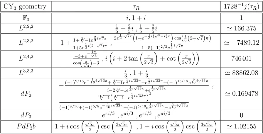
Figure 4: Urban renewal procedure focusing on a three-valent corner of the R-box. Insertion of T41

causes a two-valent node to appear, which must be removed by integrating out a massive field. This

looks like a potential problem to collapse the two white nodes into one.

The answer to the puzzle comes from looking more carefully at the linear constraints. We have already checked in the previous section, that all the charges can be assigned consistently after the urban renewal procedure (but before integration of massive fields). This means that in the situation depicted in Figure 4 the charges of fields connected to the two-valent node satisfy:

U41+T41 = 2 . (3.13)

The lengths of the corresponding edges in isoradial embedding are then:

lU41 = 2 cos

πU41

2

= 2 cos

π(2−T41)

2

=−2 cos

πT41

2

while the angle in between is

θ =πT41+U41

2 =π . (3.15)

Negative lengths are fine from the point of view of isoradial embedding; this just means that the edge extends in the opposite direction. These relationships imply that the two nodes adjacent to the two-valent node will actually be at exactly the same position in isoradial embedding! A more accurate depiction of the situation is as shown in Figure 5. This means that there is no problem with removing the two-valent node and collapsing the two — nothing else in the isoradial embedding needs to be moved, and allR-charges can be kept unchanged.

R1

R4

U41

S1

S4

S1

S4

U41 T41

Figure 5: Urban renewal and integration out of a massive field in isoradial embedding. The two nodes that need to be collapsed are already in the same position, as in the middle picture, and nothing needs

to be moved.

One final point is that the process of getting rid of two edges incident on one edge also conserves the a-function, because, using (3.13),

(U41−1)3+ (T41−1)3 = (U41−1)3+ (2−U41−1)3 = 0 . (3.16)

That means in the end, after urban renewal and integration out of the massive fields, we still end up with an assignment of R-charges that satisfies a-maximization.

For a concrete example, we illustrate the full urban renewal process in the isoradial embedding of the dimer corresponding to dP3, the Calabi–Yau cone over the third del Pezzo

surface, or_P2 _{blown up at three generic points. This is drawn in Figure 6.}

3.1.2 Physics of the assumption of local rigidity

1 2

3

4 5

6 2 1

3 4 5 6 1 2 3 4 5 6 1 2 3 4 5 6 1 2 3 4 5 6 1 2 3 4 5 6 1 2 3 4 5 6 1 2 3 4 5 6 1 2 3 4 5 6

Figure 6: Seiberg duality between phases I and II of dP3. Urban renewal is performed on face one

of the tiling. The first step flips and moves the tile and second step integrates out a massive field

thus introduced. Note two of the new fields have length zero (R = 1) and are not visible in isoradial embedding.

As a Seiberg dual pair, the original and the urban renewed theory will necessarily have the same mesonic moduli space and the same central charge. The assumption of local rigidity, as shown above, fulfills these expectations. This assumption fixes the R-charges of some of the fields of the magnetic theory — namely those untouched by Seiberg duality — to be the same as in the original electric theory. This means that the magnetic trial R-charge is not the most general one.

In order to further understand this point, let us consider the fields in the electric theory, which are untouched by the Seiberg duality and thus are mapped trivially into the magnetic theory. These fields will be either adjoints or bifundamentals of the gauge group factors which are also trivially mapped by Seiberg duality into the magnetic theory. Let us denote these fields as Xa

ij, with i, j running through those gauge groups on which Seiberg duality is not performed and a an index keeping track of their multiplicity.

Clearly, we can construct the gauge invariant chiral operators in the electric theory with baryons B[Xa

ij] = detXija if i 6= j and mesons M[Xija] = TrXiia if i = j.6 By construction, these operators are trivially mapped into the magnetic theory. On the other hand, Seiberg duality demands that the chiral ring and the set of baryonic operators are isomorphic. This means that the baryonic operatorB[Xa

ij] must have, in both theories, the same dimension and be charged under the same baryonic symmetry. As ∆[B[Xa

ij] =

3N

2 R[X

a

ij] in both theories, it is obvious thatR[Xa

ij] must be the same in both the electric and magnetic theories. Similarly, this holds for the mesonic operators M[Xa

ii], so that R[Xiia] also must be equal in the two 6_{We might imagine constructing more gauge invariant chiral operators, but for our purposes it is sufficient}

theories.

We have argued that theR-charges of fields trivially mapped under Seiberg duality must remain the same at the fixed point. We have also explained that for the theories of interest there is no mixing with accidental Abelian symmetries along the flow, and so it is consistent, for fields trivially mapped under Seiberg duality, to choose in the UV trial R-charges that are the same as in the original electric theory. This explains the assumption of local rigidity.

3.2

j

(

τ

)

is an invariant under Seiberg duality

We can now come back to our original problem of the invariance of the τR under Seiberg duality. We have just proved that urban renewal is indeed a local movement in the isoradial dimer. As such, the global structure of the dimer does not change. In particular, the unit cell of the torus where theR-dimer is drawn will not change, which immediately implies that the τR is kept invariant — up to an SL(2,Z) transformation — under Seiberg duality.

In Section 4 we shall establish the invariance of τR by considering only the toric diagram. These two sections provide a purely field theoretic argument for the invariance of τR among Seiberg dual phases. However, it is interesting to explore the string theoretic perspective on this. We will postpone such an analysis to a forthcoming publication [33].

4

τ

from toric data

In Section 3, we have analyzed the urban renewal procedure and shown that the global structure ofR-dimer is unchanged, which keepsj(τR) invariant between Seiberg dual phases. In this section we take one more step and show how it is possible to computeτRdirectly from the toric diagram, bypassing the construction of specific dimers altogether. For this purpose we will use the formulation of a-maximization based purely on the toric data as in [35, 36].

Note that by the arguments of this section the invariance of j(τR) would appear trivial, because no information about the dimer is used in the calculation, only the toric diagram. However, there seems to be some uncertainty [27], as to whether the methods of [35, 36] apply to any phase of the theory or just the so-called minimal phase, which is the one with the fewest perfect matchings in the brane tiling. In this light, our explicit comparison of phases in Section 3 gives us encouragement to propose that the calculation in this section is, in fact, valid for any phase. We will attempt to further clarify this point in the following discussion.

4.1

a

-maximization from toric diagram

First, we use the method of [35, 36] to write the trial a-function directly from the toric diagram. In order to do that we assign a variable ai to each external point of the toric diagram (see Figure 7). There is a single constraint

a1

a2

a3 a4 a5

b5

b₁

b2

b3 b4

H1, 0L

H0,-1L

H0,-1L

H0, 1L

H-1, 1L

Figure 7: The toric diagram for SPP. Each external point has a variableaiassigned, and each primitive

normal has variablebi. The (pi, qi) numbers of primitive normals indicate the winding numbers of the

corresponding zig-zag paths.

t

X

i=1

ai = 2 (4.17)

leaving t−1 independent variables, where t is the number of external points in the toric diagram. This is the number of non-anomalous U(1) symmetries and thus the expected number of variables for a-maximization. The geometric meaning of these variables is more clear if we consider corresponding variables for the primitive normals:

b1 =a1 , b2 =a1+a2 ,

bi = i

X

j=1 ai ,

bt= 2 .

(4.18)

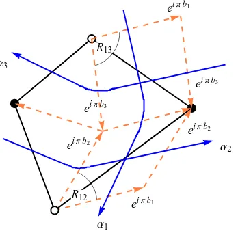
the fact that a zig-zag path always crosses rhombi through opposite edges, which are parallel, and so all the edges that the zig-zag path crosses are parallel with direction parameterized bybi. Note that we assign a direction to the rhombi edge such that the arrow points to the left looking down the zig-zag path direction. Finally, it will be useful to think of the plane of the tiling as the complex plane, in which case the vectors corresponding to the rhombi edges, all having length one, are written as eiπbi_.

Α1

Α2

Α3

eiΠb1 eiΠb1

eiΠb3 eiΠb3

eiΠb2 eiΠb2

R12 R13

Figure 8: Zig-zag paths and rhombi. Blue lines αi indicate zig-zag paths and orange lines are rhombi

edges with assigned direction. The vectors of all rhombi edges intersected by the sameαi are equal and

parameterized asexp(iπbi).

Now, given the parameterization, the triala-function is constructed as follows. Every edge of the tiling is at an intersection of two zig-zag paths αi,αj. If we adopt a convention that on the intersection αj is counter-clockwise from αi, then the R-charge of the corresponding field, as can be easily read off from the diagram, is

Rij =bj−bi =ai+1+ai+2+. . .+aj . (4.19) We have to be careful when we go around the diagram, and since in our current convention (4.18) bi are increasing, we have to take for j < i:

Rij = 2 +bj−bi =ai+1+. . .+at+a1+. . .+aj . (4.20) Having parameterized all field charges in terms of bi and knowing that for every intersection of the zig-zag paths there is a corresponding field, it is easy to write the a-function [35, 36]:

a(bi) = 9 32

 F +

X

i,j,hwi,wji>0

hwi, wji(Rij −1)3



whereRij is (4.19) or (4.20) depending on whetheri < j. Herewi = (pi, qi) are the primitive normal vectors of the toric diagram and

hwi, wji ≡det

pi qi

pj qj

!

. (4.22)

The sum is performed only over hwi, wji>0 meaning wj is counter-clockwise from wi. So, maximizing thisa(bi) as a function oft−1 variables we get the preferred isoradial embedding and the trueR-charges for all fields using (4.19), (4.20).

Before continuing on, let us briefly discuss how dual phases are related from the per-spective of this construction. The difference turns out to be in how many times any two zig-zag paths αi, αj actually intersect. Given their winding numbers wi, wj, we know that they have to intersect at least hwi, wji times, but it could be more. For example, it can be seen that during urban renewal four new intersections are introduced between zig-zag paths7

corresponding to four new fields in Figure 2. It might then seem that (4.21) is assuming a minimal model, where the number of intersections is precisely hwi, wji. However, on closer inspection it turns out that this is not the case. Whenever extra intersections between zig-zag paths are introduced, they always come in pairs of opposite orientations: one where

αj is counter-clockwise from αi and a second one vice-versa. Expressions (4.19), (4.20) for

R-charges can still be trusted in this case and we can see that the charges of the two extra fields are related (here assuming i < j):8

Rij +Rji = (bj −bi) + (2 +bi−bj) = 2 . (4.23) This in turns shows that the a-trial remains unchanged:

∆a= 9

32 (Rij −1)

3_{+ (R}

ji−1)3

= 9

32 (Rij −1)

3_{+ (2−R}

ij −1)3

= 0 . (4.24)

In other words, the coefficient in front of (Rij −1)3 in (4.21) is not the total number of intersections between αi and αj, but the sum of oriented intersections, which is always

hwi, wji. Therefore (4.21) is valid for all, and not just for minimal models.

4.2

Explicit

τ

and two-dimensional

a

-maximization

Now that we have bi that maximize a-trial it is in fact possible to write down an explicit formula for τR. Let us consider the rhombus lattice on the complex plane in Figure 8. We take it to be periodically identifiedz ∼z+c∼z+cτR. Now if we follow a zig-zag path with

7 _{See, for example, Figure 25 of [44].}

8 _{Note that this corresponds to a relation likeT}

winding numbers (p, q) until we reach an identified point, the displacement on the complex plane is

∆z(p,q)=c(p+qτR) . (4.25) On the other hand, we can calculate the displacement from the parameters bi. Take as an example the zig-zag path α1 in Figure 8. As the zig-zag path crosses each rhombus, it

intersects another path αi. As can be seen from the figure, the displacement after crossing the rhombus is given by the edge parallel to α1, which is justeiπbi, wherebi is the parameter associated with the intersected path αi. More precisely the displacement is ∆z = −eiπbi if the intersection is positive (that is αi is counter-clockwise from α1) and ∆z = eiπbi if

negative. For example, one can see that the displacement is eiπb3 _{after intersection with}

α3 and it is −eiπb2 after intersection withα2. Therefore, the total displacement after going

around a zig-zag path (p, q) is

∆z(p,q)=w =− t

X

i=1

hw, wiieiπbi (4.26)

because hw, wii is the number of positive intersections (minus the number of negative) with each pathαi.

Now we can pick two zig-zag paths (pa, qa) and (pb, qb), apply (4.25): ∆z(pa,qa)

∆z(pb,qb)

= pa+qaτR

pb+qbτR =

P

ihwa, wiie iπbi

P

ihwb, wiieiπbi

, (4.27)

and solve for τR. The answer, of course, should not depend on which two paths we pick. We find indeed that it doesn’t, and the result is a compact expression for τR in terms of the toric data and bi:

τR=−

P

ipie iπbi

P

iqieiπbi

. (4.28)

Note, by the way, this is just τR = ∆z(0,1)/∆z(1,0), even though we cannot guarantee that

paths (0,1) and (1,0) always exist.

According to [35] the maximization of a(bi) in (4.21) over a (t−1)-dimensional space can be further reduced to a two-dimensional maximization ofa(x, y). In this section we begin to examine the interplay of (x, y) parameterization of the isoradial embeddings andτR.

(x, y) we can assign trial ai charges as:

ai(x, y) =

2li(x, y)

P

jlj(x, y)

, (4.29)

li(x, y)≡

hvi−1, vii

hri−1, vi−1ihri, vii

, (4.30)

ri(x, y)≡Vi−(x, y), (4.31)

vi ≡Vi+1−Vi . (4.32)

HereViare the coordinates of toric diagram’s external points,viare the vectors along external edges, and ri are vectors from the point (x, y) to the external points. If we now use these

ai(x, y) to write the fulla-trial function through (4.18) and (4.21), we get a functiona(x, y), which, when maximized gives the same ai as the full function a(bi). For the details and the proof of this statement see [35].

An interesting observation is that at any point in the parameter space (x, y), we can apply (4.28) to get a function τR(x, y) over the interior of the toric diagram. Since τR also has two real parameters it is plausible that we can invert the function and in the end express

a-trial purely as a function ofτR andτR. This would translate to the maximization ofa(τR) over the space of complex structures which might have some nice geometric interpretation. For now, let us content ourselves with the example of _C3_{. From its details in Appendix A,}

we see that τR= −1+e 2πiy

1−e−2πix, so that upon inverting we have e2πix =

τR+τRτR

τR+τRτR and e

2πiy ₌ 1+τR

1+τR.

Whence, we have the desired formula of the trial a-function as

atrial = 27 4(2πi)3 log

τR+τRτR

τR+τRτR

log

1 +τR 1 +τR

(2πi−log

τR

τR

) , (4.33) to be maximized over the parameters τR and τR.

5

a

-maximization and invariants in terms of

general-ized incidence matrix

Encouraged by the discovery that τR is invariant under Seiberg duality, a quantity undis-cussed in field theories prior to [30, 31], we now turn to the search for more invariants. To this end, we will first examine a-maximization from a new perspective.

5.1

Lagrange multipliers and

a

-maximization

E, F, V, we must maximize

a =X i∈E

(Ri−1)3 , (5.1)

subject to two conditions. 1. For each face F, we have

X

i∈∂F

(1−Ri) = 2 , (5.2)

with the sum over edges that bound the face F. The condition i ∈∂F indicates that edge i is in the boundary of face F.

2. For each vertex V we have

X

i∈∂−1_V

Ri = 2 , (5.3)

with sum over edges incident on V. The condition i ∈∂−1_{V indicates that the vertex} V has the edgei incident on it. It is also useful to recast this as

X

i∈∂−1_V

(1−Ri) = dV −2, (5.4)

where dV is defined as the valency of the vertex, i.e., the number of edges incident on the vertex, thus, dV :=

P

i∈∂−1_V 1.

If we apply the usual technique of solving the linear constraints, then substituting back into the cubic and extremizing, we could have complicated polynomials. We now use the La-grange multiplier method which, as will be shortly seen, allows for some nice simplifications. Define the standard function

A = d

X

i=1

(Ri−1)3+

X

F

λF(2−

X

i∈∂F

(1−Ri)) +

X

V

λV(2−

X

i∈∂−1_V

Ri)

= d

X

i=1

(Ri−1)3+

X

F

λF(2−

X

i∈∂F

(1−Ri)) +

X

V

λV((dV −2)−

X

i∈∂−1_V

(1−Ri)), (5.5) where we have explicitly marked the sumi∈E by denoting the total number of edges asd. The Lagrange multipliers for each V and for each F is denoted respectively as λV and λF.

To extremize A, we need to set to zero the partial derivatives for each edge (field) i,

∂RiA= 3(Ri−1)

2 ₊ X

F:i∈∂F

λF +

X

V:∂(i)=V

which will always give us quadratic equations for Ri, with the coefficients involving the multipliers λV, λF, which will be determined by solving the constraints at the end. Each edge bounds two faces, call them F_i+, F_i−, and two vertices V_i+, V_i−.

A cleaner way to write the equations (5.6) is to define ageneralized incidence matrix, which we call M. Usually, incidence matrices are defined for graphs, which have edges and vertices. Here we have an embedded graph, which has edges, faces, and vertices. The matrix

Mij has the row index i running over the list of vertices and faces. The index j runs over the edges.9 _{Since we have |V|+|F| − |E|= 0 from Euler’s theorem applied to a genus one}

Riemann surface, this is remarkably a square matrix. When i is a vertex V, the entries of

Mij are 1 or 0, depending on whether the edge j ∈ ∂−1V or not. This part of M is just the incidence matrix of the graph. When i is a face F, then the entry of Mij is 0 if the edge j does not bound the face, 1 if the edge j appears once as the boundary of the face is traversed, and 2 if the edge appears twice (once from each side). The last happens whenever

i transforms as an adjoint field under the gauge group corresponding to F rather than as a fundamental or antifundamental.

There is another nice way to interpret the matrix M, namely, in terms of the associated rhombus lattice [28]. In the mapping from dimer to rhombus lattice edges turn into faces (rhombi) while both faces and vertices turn into vertices. The two adjacent faces and two adjacent vertices to a given edge in the dimer become the four corners of the rhombus. Therefore Mij is 1 precisely if rhombus j has vertex i as a corner and 0 otherwise. It can also be 2 if the same vertex appears in two corners of the rhombus due to periodicity.

We can therefore write

∂RiA= 3(Ri−1)

2₋ X

k∈{V,F}

λkMki . (5.7)

Let us also define

µi = (1−Ri) . (5.8)

Then the condition ∂RiA = 0 becomes, rather succinctly,

3µ2_i = X k∈{V,F}

λkMki . (5.9)

9 _{Such structures have a history in the mathematics literature (see, for example, [45]). We can define}

a rectangular matrix Π(2) _{whose columns are faces and whose rows are edges, and the entry Π}(2)

ji counts

the number of times the edgej bounds the facei. Similarly, we can define another rectangular matrix Π(1) whose columns are edges and whose rows are vertices, and the Π(1)_ij is zero or one depending on whether the

vertexiis an endpoint of the edgej. The matrixMwe have constructed combines these as Π

(1)

t_Π(2) !

The linear constraints can also be written elegantly in terms of the incidence matrix M. To do this we would like to package (5.2) and (5.4) into a single equation. To this effect, define a vector Di, where i runs over faces and vertices. When i corresponds to a face, we put Di = 2. When i corresponds to a vertex, we put Di = (di−2), where di is the valency of the vertex.

Note that the vector Di carries no additional information beyond what is already in the matrix Mij. Wheni corresponds to a vertex, the sum over edges j

d

X

j=1

Mij =di =Di+ 2 , (5.10) as the total number of non-zero entries equals the number of edges that emanate from the vertex. When i corresponds to a face, the corresponding element of the vector Di is always 2, and so conveys no new information.

Now, the two equations (5.2) and (5.4) can be written as

X

j∈E

Mijµj =Di , (5.11)

with the sum on j running over all the edges, 1, . . . , d. Typically the d equations (5.11) are not independent. Rather, the number of independent equations is equal to the rank of the matrix:

Rank(M) =d− |Ker(M)| , (5.12) where Ker(M) is the space of null eigenvectors of M given by the eigenvectors with zero eigenvalues.

This suggests that the null eigenvectors of M contain useful information about the R -charges. Suppose Na

i is a null eigenvector, where a runs over the possible null eigenvectors and i runs over the d components. From the definition of null eigenvector, we have

X

j

MijNja= 0 . (5.13)

Using this in (5.9), we obtain

X

i

µ2_iNa i =

X

k

λkMkiNia= 0 . (5.14) In fact, if we consider the set of equations

d

X

j=1

Mijµj =Di , d

X

i=1 µ2_iNa

i = 0

we have precisely d equations for d variables, thus allowing us to find the R-charges via

Ri = µi + 1. As argued in [36] from the gravitational dual perspective, there is in fact a unique solution to the a-maximization problem. In our case, the solution set of the boxed equations will give us the R-charges which maximize a upon imposing the unitarity bound

R≥ 2

3 for gauge invariant operators. In fact, for practical purposes, the weaker requirement R >0 is enough to select the correct R-charge assignments.

5.2

Properties of the generalized incidence matrix

It is useful here to make the connection with rhombi and zig-zag paths again. It is a well known fact [28] that the number of independent trial R-charges after solving the linear constraints is (t−1) where t is the number of external points in the toric diagram of the theory. We can also see this explicitly from the zig-zag paths on the dimer. Every consistent dimer has t zig-zag paths and the remaining (t−1) variables in the trial a-function can in fact be associated with the (t−1) paths which are linearly independent (in the appropriate sense mentioned below). It is therefore nice to see these zig-zag paths appear naturally here: they are precisely the null vectors Na

i of matrix M!

Let us elaborate on what this means. First, we assign ad-dimensional vector to a zig-zag path αa in the dimer as follows:

Na i =

        

+1 if αa intersects edgei after turning right at a node

−1 if αa intersects edgei after turning left at a node 0 if αa does not intersect edgei

. (5.16)

The overall sign does not matter. The point is that edges are included with alternating signs. This vector, in fact, represents the charge assignments of the baryonicU(1) symmetry associated with αa.

We can prove that suchNa

i is a null vector ofM. Consider

P

jMijN a

j for a fixediwhich is now either a face or a vertex. Going to the rhombus lattice picture, the zig-zag path is a sequence of rhombi with alternating signs (otherwise known as “rhombus path” or “train track”), whilei is a vertex. The sum simply counts how many times the vertexiis included in positive faces minus the negative faces, but since each vertex is included in precisely two adjacent faces, the sum will be zero for all i (see Figure 8 in [28]). Therefore, Na

i is a null vector. Now, to show that vectorsNa

i in fact cover the whole Ker(M) we simply cite the fact that there are (t−1) independent Na

i among the t zig-zag paths, corresponding to (t−1) anomaly free U(1) symmetries. A single relationship between them is that Pt

a=1N

a i = 0, because each edge is included twice with opposite signs. In the end if we takeNa

In conclusion, our generalized adjacency matrix has the property that

|Ker(M)|=t−1 , (5.17)

wheretis the number of external points in the toric diagram. An immediate corollary of this is that |Ker(M)|, a rough measure of the complexity of the R-charges as it is the number of quadratic equations, is preserved under Seiberg (toric) duality since it depends only on the toric diagram. One can easily verify this and for reference, we tabulate the results in Table 2.

CY3 geometry |Ker(M)|

F0 3

L2,2,2 5

L2,3,2 ₆ L2,4,2 ₇ L3,3,3 7

dP2 4

dP3 5

P dP3b 5

Table 2: The dimension of the null space of the matrixMis the same for all the Seiberg dual phases of a dimer theory.

Another visual and interesting consequence from|Ker(M)|can be obtained by summing overi in (5.13). Indeed, it happens that Pd

i=1Mij = 4 because a fixed edge j must connect two vertices, a black and a white node from the bipartite condition, and as well separates two faces (which might be the same). As P

i Mij is independent on j, it then follows that

P

j Nja = 0 for all a. Thus, we might think of them as defining the gauged linear sigma model (GLSM) charges for a Calabi–Yau variety. The role of this variety, which can be seen experimentally not to be invariant under Seiberg duality, is not clear.

Summing the first equation in (5.15) over i, we may conclude that d

X

i,j=1

Mijµj = d

X

i=1

Di = 4|F| . (5.18)

5.3

Applications:

_C

and SPP

C3 calculation: In this case

M=

  

1 1 1 1 1 1 2 2 2

 

 , D=   

1 1 2

 

 . (5.19)

The first row corresponds to the black vertex, the second to the white vertex, the third to the face. The 2 corresponds to the fact that as the boundary of the face is traversed, we encounter each edge twice; that is, all three fields here are adjoints.

In this case two linearly independent null vectors are

N(1) =

  

1 0

−1

   , N

(2)

=

  

0 1

−1

 

 . (5.20)

Using these null vectors, the second of (5.15) leads to equations

µ2₁ =µ2₂ =µ2₃ . (5.21) Next, the first equation in (5.15) gives

µ1+µ2+µ3 = 1 . (5.22)

Hence, combining (5.21) with (5.22) and demanding that the R-charges be positive, we retrieve the familiar result that for all i= 1,2,3,

µi = 1

3 , Ri = 2

3 . (5.23)

Note that, as promised, the sum of the entries of each N vector is zero. This ensures that when we take the quotient _C3_//Na,†_{, we have a Calabi–Yau space. As we have stated,} the null vectors can be thought of as the set of charges defining the GLSM for the resulting Calabi–Yau variety. Taking Ker(Na,†_{), this is one-dimensional and therefore}

C. We can

understand this as follows: N(1) _{yields an identification z}

1 ∼ −z2 while N(2) yields an

identification z2 ∼ −z3. Thus, we are left with one coordinate.

matrix M, and the D vector are, respectively, 2 3 1 2 3 1 2 3 1 2 3 1 1 2 1 2 1 2 1 2 M=             

0 0 1 1 0 0 1 1 1 0 0 1 1 0 0 0 0 0 1 1 1 1 1 1 1 0 0 0 1 1 1 1 0 0 0 1 1 0 0 1 1 0 0 0 1 1 1 1 2

            

, D=

             1 2 1 2 2 2 2              . (5.24)

The first row corresponds to the first black vertex, which is trivalent and so has three entries equal to 1. The second row is the second black vertex of valency four and four entries of 1 at the corresponding edges. The third and fourth rows correspond to the white vertices. The fifth, sixth, and seventh rows correspond to the three faces. The columns correspond to the fields {X12, X21, X13, X31, X23, X32, X33}.

There are four null vectors:

{N(1)_,N(2)_,N(3)_,N(4)_}=

             1 −1 0 0 0 0 0              ,              0 0 1 −1 0 0 0              ,              0 0 0 0 1 −1 0              ,              1 0 −1 0 −1 0 1              , (5.25)

corresponding to the fact that SPP has t= 5 external vertices in the toric diagram

Note that just as in (5.20), the null vectors in (5.25) have elements that sum to zero. In this case the corresponding Calabi–Yau is a conifold. (The first three null vectors reduce_C7 to_C4 and the fourth relates the coordinates of _C4 by the conifold relation.)

The first three null vectors offer the equations

µ2₁₂ =µ2₂₁ , µ2₁₃ =µ2₃₁ , µ2₂₃ =µ2₃₂ . (5.26) The last null vector though does not give a linear equation, but, rather, a quadratic:

µ2₁₂−µ2₁₃−µ2₂₃+µ2₃₃= 0 . (5.27) From the M ·µ=D we obtain three equations:

µ13+µ31−µ33= 1 ,

µ23+µ32+µ33 = 1 . (5.28)

Solving this system of equations, there are ten sets of solutions for the µij, of which only one has all of the R-charges being positive. This reproduces the known charges of the fields of SPP:

R12 =R21= 1−

1

√

3 ,

R13 =R31=R23 =R32=

1

√

3 ,

R33 = 2− √2

3 . (5.29)

We have applied this technique to all the consistent theories in the classification of [42] and find complete agreement with the the traditional methods. This shows that the solution of theR-charges can be simply expressed in terms of the generalized incidence matrix in terms of the two equations (5.15). The simple consideration in (5.12) suggests that the number of independent equations in (5.15) is exactly the right number to give all the R-charges.

6

Number theoretic invariants of Seiberg duality

We have established in Section 3 that τR is an invariant under the urban renewal operation that implements Seiberg duality on a dimer. The master space, which is the solution to the F-term equations of an N = 1 supersymmetric gauge theory, matches the IR moduli space of a quiver gauge theory [14]. Its dimension isF + 2, where F is the number ofU(N) gauge groups, i.e., the number of faces in the dimer. Generically, this master space is reducible and separates into pieces of different dimensionality. The maximal dimensional piece of the variety — the coherent component or equidimensional hull under a primary decomposition — is an (F + 2)-dimensional Calabi–Yau cone. The dimension of the coherent component is also invariant under Seiberg duality [15]. Motivated by our discussion of R-charges, in this section we scan for further new invariants of Seiberg duality.

It has been observed before that the R-charges determined bya-maximization are alge-braic numbers. These are numbers which are roots of polynomials with coefficients that are rational, i.e., belonging to _Q. The collection of all algebraic numbers forms_Q, a field closed under addition and multiplication, and obeying the relevant axioms.

Since the R-charges after Seiberg duality are obtained simply by leaving a subset of the

unchanged. So we have additional number theoretic invariants under Seiberg duality (along with j(τR)).

Indeed, the R-charges of our theories are algebraic numbers, arising from systems of polynomials, duringa-maximization, in integer coefficients. The gravity dual statement that the volume of the Sasaki–Einstein manifolds are algebraic is discussed in [46].

It is an interesting question to ask in what precise number field do the R-charges live. After all, Grothendieck’s original intent in studying the dessin d’enfants, which are an equiva-lent description of our dimer models [30,31], was to investigate the absolute Galois group [47]. The absolute Galois group Gal(_Q/_Q) acts as a symmetry of the field of algebraic numbers, which preserves the rational numbers. Moreover, it acts faithfully on the set of dessins.

For_C3, we have that theR-charges, given in (5.23), are still in_Q. For SPP, theR-charges, given in (5.29), are in_Q[√3], the rationals adjoining a single radical, viz.,√3. Recalling that the degree of a field extension K overL, commonly denoted as [K :L], is the dimension of the vector space when writing elements of K as vectors with entries inL and with basis as the numbers introduced in the extension, the degree of the minimal field extension for SPP turns out to be two.

It is instructive to tabulate the minimal number fields over the rationals wherein the

R-charges reside, for the 42 consistent dimers/tilings catalogued in [42]. In Table 3, we list the degree of extension, starting from the trivial degree one, when the R-charges are rational.10 _{For completeness, we shall use the pair notation (theory, minimal field containing}

the R-charges). We point out that L1,1,1 _{is commonly known as the conifold, L}1,2,1 _{as SPP,}

and _C3_/

Z3 asdP0.

Table 3 shows that different theories in fact have the same field extensions. Note, for instance, that at degree one, we have_C3, the conifold, various orbifolds of these theories and

Z3,1, which is not related to the others. At degree two, we have another orbifold example:

L2,4,2 has the same R-charges as the parent L1,2,1 and thus the same field extension. That

L1,3,1 has the same field extension as L2,3,2 is more interesting. In general, La,b,a and Ld,b,d

with d = b− a have identical fields extensions. Indeed, this can be easily seen from the 10 _{In the last entry in Table 3,f(x) is:}

129895959052919063627088658824484033170106970563057053464097738113158357486077961163576360759355431959070613052958136429700−

7990706677245120266223000216858808331489576634388895611486208 + 812780867079221751989485691592256982562445490116486994857815−

32406074736034254990618952381740902301999847184924691931671841243521462114222422531961018099657867264x−1605590251086677055−

032517976888916263032528341347296581174611981547691619152719002618787800157726841563671420301829401419343371688614035456x2−

58501895038049041480240324513991980662242406126145870387880078437110541099265053803105661755970304429347559234666496x3+ 694785402847564626838097983555518880082522398594151133211393984791686345118886967099469533184x4+

8748375862087189421259901955556860436477229485948805897674628434108672x5−68749725604677082362249064632675381493544491440x6−

162855999849603150949559x7+x8,