1
Load-cell based characterization system for a ‘Violin-Mode’
shadow-sensor in advanced LIGO suspensions
N.A. Lockerbie and K.V. Tokmakov
SUPA (Scottish Universities Physics Alliance) Department of Physics, University of Strathclyde, 107 Rottenrow, Glasgow G4 0NG, UK.
Abstract. The background to this work was a prototype shadow sensor, which was designed for retro-fitting to an Advanced LIGO (Laser Interferometer Gravitational wave Observatory) test-mass/mirror suspension, in which 40 kg test-test-mass/mirrors are each suspended by four approximately 600 mm long by 0.4 mm diameter fused-silica suspension fibres. The shadow sensor comprised a LED source of Near InfraRed (NIR) radiation, and a rectangular silicon photodiode detector, which, together, were to bracket the fibre under test. The aim was to detect transverse Violin-Mode resonances in the suspension fibres. Part of the testing procedure involved tensioning a silica fibre sample, and translating it transversely through the illuminating NIR beam, so as to measure the DC responsivity of the detection system to fibre displacement. However, an equally important part of the procedure, reported here, was to keep the fibre under test stationary within the beam, whilst trying to detect low-level AC Violin-Mode resonances excited on the fibre, in order to confirm the primary function of the sensor. Therefore, a tensioning system, incorporating a load-cell readout, was built into the test fibre’s holder. The fibre then was excited by a signal generator, audio power amplifier, and distant loudspeaker, and clear resonances were detected. A theory for the expected fundamental resonant frequency as a function of fibre tension was developed, and is reported here, and this theory was found to match closely the detected resonant frequencies as they varied with tension. Consequently, the resonances seen were identified as being proper Violin-Mode fundamental resonances of the fibre, and the operation of the Violin-Mode detection system was validated.
PACS numbers: 04.80.Nn, 84.30.-r, 06.30.Bp, 07.07.Df, 07.57.-c
1. Introduction
A system of four shadow-sensors was designed to be retro-fitted to an Advanced LIGO (or aLIGO, where the acronym LIGO stands for Laser Interferometer Gravitational wave Observatory) test-mass/mirror suspension, in which a 40 kg test-mass is suspended by four fused silica fibres, the dimensions of the fibres being approximately 600 mm long by 0.4 mm in diameter [1–8]. These shadow-sensors—one per suspension fibre—each comprised a ‘synthesized split-photodiode’ detector of shadow displacement, and a Near InfraRed (NIR: = 890 nm) source of collimated illumination—this casting a shadow of the illuminated fibre onto the facing detector [9,10,11]. The principal purpose of the full detection system was to monitor any lateral ‘Violin-Mode’ resonances that might be excited on these fibres [12], such that this oscillatory motion then could be cold-damped, actively [13].
A characterization test-rig was constructed that could vary the tension in a short (~70 mm long) fused silica fibre test sample, in order that the main function of the optical shadow-sensing system could be tested at appropriate frequencies. The fibre was illuminated by the NIR source, and the Violin-Mode shadow-sensor’s output was monitored continuously, as the tensioned fibre sample was excited acoustically across a band of frequencies in the audio range, in order to flag-up any sympathetic VM resonances that might manifest themselves at the acoustic driving frequency.
2 the detected resonant frequencies of the fibre under test were inter-compared with this theory, as a function of the fibre’s tension.
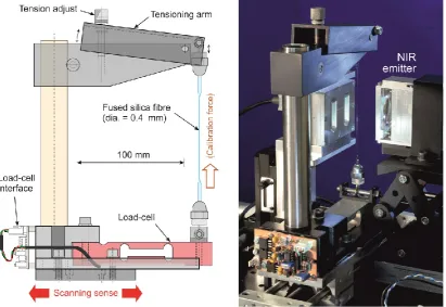
Figure 1. The fibre translation system, constructed on an optical plate (with 45° corners), this plate being separated from the—slightly larger—base of a steel screening case (measuring 500 mm 500 mm 330 mm high, with a 1.7 mm wall thickness) by four Sorbothane vibration-damping feet. The steel base was itself separated from the optical table by four additional Sorbothane feet. The case also had steel lid, so as to seal it fully electrostatically (it was earthed), magnetically (being ferromagnetic), and optically—being light-tight.
[image:2.595.128.498.103.390.2] [image:2.595.103.515.467.750.2]
3 to the base of the fibre responded to the applied tension, and the load-cell interface (seen in Figure 3) provided a voltage analogue of the tension in the fibre. Right: photo of the mounted fibre sample positioned between the NIR emitter (at right) and its facing shadow sensor—located in a dual ‘split-photodiode’ detector housing. The detected resonant frequencies of the test fibre were found to follow quite closely the theory developed here, over a range of fibre tension spanning 43.5 grammes weight ( 0.427 N)–1.005 kg.wt. ( 9.86 N). Consequently, the resonances seen were deemed to have been proper fundamental VM resonances of the test fibre, thereby validating the function of the Violin-Mode detection system.
2. The load-cell based fibre monitoring system
2.1. The Violin-Mode detection system
VM resonances of the actual aLIGO suspension fibres were known to have fundamental resonant frequencies ~500 Hz, and the shadow-sensors themselves, including the transimpedance amplifier connected to each ‘synthesized split-photodiode detector,’ were required to have an AC Violin-Mode bandwidth which extended from below this frequency up to above 5 kHz, in order to cover (at least) the 10th harmonic. The bandwidth of the
as-built detection system was measured to extend from 226 Hz to 8.93 kHz (at its 3 dB points), in fact. In addition, the transimpedance amplifier possessed two ancillary DC outputs—one coming from each of the two photodiode (PD) elements in its ‘split-detector’—and these assisted in the initial alignment of the fibre’s shadow onto the centre of the shadow-sensing detector [14,15].
2.2 The fibre positioning (and scanning) system
The scanning system, which has been described elsewhere, is shown in Figure 1 [16]. Here, it was used only for the initial positioning of the fibre. The fibre test sample, orientated vertically, was mounted into its holder, as shown in Figure 2, such that it was kept under tension. The fibre, in this holder, then was attached to the sliding carriage of the scanning system shown in Figures 1 and 2. This carriage allowed for controlled movement of the fibre in a direction orthogonal to that of the illuminating NIR beam, the position of the fibre being sensed with a resolution of ±1 m by a linear magnetic encoder. In this way, the fibre’s lateral position was adjusted relative to the fixed illuminating beam, so that the fibre’s shadow fell accurately onto the centre of the detector.
2.3 The fibre tensioning system
The fibre’s ‘bespoke’ tensioning apparatus is shown in Figures 2 and 3. Figure 2 shows how a mechanical tensioning arm could be adjusted via a knurled screw, this having a fine-pitched thread, and an asymmetric lever-arm, in order to make fine adjustments to the tension in the fibre. The lower end of the fibre was attached to a temperature-compensated TEDEA HUNTLEIGH single-point Model 1022 load-cell, this having a 10 kg.wt. ( 98.1 N) Full Scale—consequently tensions will be expressed here in kg.wt. force units. 2.4 Tension conditioning electronics
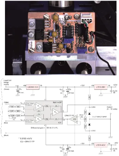
4 25-turn, potentiometer—connected here as a variable resistor. This arrangement allowed the voltage gain of IC1 to be trimmed with high precision (±1.4% about its nominal mid-value of 521.8), as indicated. Similarly, the bandgap-derived voltage input from the wiper of the 10 k, 25-turn, potentiometer, connected to IC2, allowed the voltage offset of the interface to be adjusted with high precision (and stability), over a narrow range of ±49 mV.
Figure 3. The load-cell amplifier interface. At top: Photo of the interface (as constructed using a ground-plane on a double-sided PCB measuring 64 mm 40 mm), mounted directly onto the sliding carriage, adjacent to the load cell (as shown in Figure 2). At bottom: circuit diagram of the interface to the TEDEA HUNTLEIGH Model 1022 single-point load-cell (Full Scale = 10 kg.wt.). A ±20 V bench PSU powered the interface unit. Please refer to Figure 4 and the text for details of the gain and offset capabilities of this circuit.
2.5 Calibration of and results from the tension conditioning interface
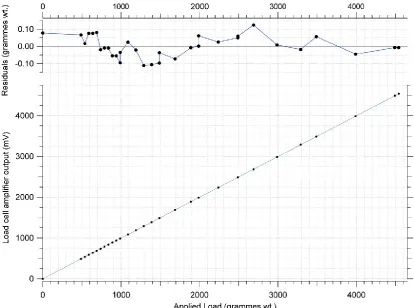
[image:4.595.123.505.129.629.2]5 suspended by fine nylon lines from the fibre attachment point on the load-cell. In this way, adding successive weights to the pan increased the applied—vertically downward—load applied to the load-cell. Before being added to the loading pan (of known weight) the standard weights were each weighed accurately using a precision Sartorius balance, this having a 5.2 kg full scale, and a 10 mg resolution. Following small adjustments to its differential gain and offset, the slope of the best-fit calibration line for the Load Cell amplifier was found to be (1.00000 ± 8 106) volts/kg.wt., with an intercept of 0.0785 ±
[image:5.595.112.527.184.492.2]0.0184 mV (i.e., close to 0.08 grammes wt.). Please refer to Figure 4 for the actual calibration results.
Figure 4. Calibration of the load cell amplifier circuit shown in Figure 3, over the range 0–4.54 kg.wt. A set of Class M1 standard brass weights were used for this calibration. The slope of the best-fit calibration line for the Load Cell amplifier = (1.00000 ± 8 106) V/kg.wt., with an intercept = 0.0785 ± 0.0184 mV (i.e., close to 0.08 grammes wt.). Please see text for details of the calibration procedure.
3. Detecting fibre resonances
3.1 Acoustic excitation measurements: method
6 The fibre then was excited acoustically, using a Stanford Research Systems DS345 signal generator, driving a 4 7" diameter, loudspeaker (rated at 350 W, and placed at a distance of ~1.5 m from the fibre’s closed steel enclosure), via a SoundMaster VF 250 power amplifier. However, a relatively low amplitude of sinusoidal signal was used to drive the loudspeaker, and the sound level in the vicinity of the steel enclosure was only ~75–80 dB. In practice, the source of sound was swept in frequency slowly across the audio range, and, simultaneously, the spectrum of the amplified signal from the photodiode detector was monitored, using a Stanford Research Systems SR785 Dynamic Signal Analyzer. The resulting spectrum was observed continuously, in order to flag-up any candidate VM
[image:6.595.54.557.290.547.2]resonances that might manifest themselves at the driving frequency. Once a resonance was detected, the loudspeaker’s driving frequency was adjusted to match the peak of the resonance, and the spectrum was measured, and recorded. Please note that upon sweeping the drive frequency no other peaks ever were seen, above the background noise level, in the vicinity of the main resonances. The fibre’s tension then was adjusted to a new value, and the procedure was repeated. It was found in practice that the applied tension sometimes decreased slightly over time, and this was traced eventually to slippage in the fibre’s end fixings—for which a rigid epoxy would have been a better choice.
Figure 5. Power (amplitude) Spectral Density as a function of frequency, measured at the AC output of the Violin-Mode (VM) amplifier, under different conditions of illumination, acoustic excitation, and fibre Tension. Green/blue traces (63 dBVrms/Hz at 1 kHz): fibre’s shadow not falling onto the detector. Black trace (64.4 dBVrms/Hz at 1 kHz): fibre’s shadow falling over the centre of the ‘split-photodiode’ detector, but no acoustic excitation. Resonances of the steel enclosure are seen at frequencies below approximately 300 Hz. Red trace: fibre excited acoustically by the loudspeaker at a frequency of 936 Hz, for a fibre tension of 0.436 kg.wt. Blue trace: fibre’s tension was increased to 0.712 kg.wt., and the fibre’sresonance was seen to increase in frequency to 1110 Hz.
3.2 Results from the acoustic excitation measurements
The green/blue traces (63 dBVrms/Hz at 1 kHz) in Figure 5 show no resonances, since here the
shadow of the fibre fell slightly to one side of the detector. The roll-off towards low frequencies of the amplifier’s VM passband is apparent, however. In contrast, the black trace in the Figure (64.4 dBVrms/Hz at 1 kHz) had the fibre’s shadow falling over the centre of the
7 actually reached a peak of 36 dBVrms/Hz, at 48 Hz. For the red trace in the Figure the fibre
was excited acoustically by the distant loudspeaker, and an additional, clear, resonance is seen at a frequency of 936 Hz. The tension in the fibre was measured here to be 0.436 kg.wt. The fibre’s tension then was increased to 0.712 kg.wt. (blue trace), and the resonance is seen to have increased in frequency, to 1110 Hz: the resonances’ quality factor was Q > 500. The measured resonant frequencies have been plotted as a function of fibre tension in Figure 6.
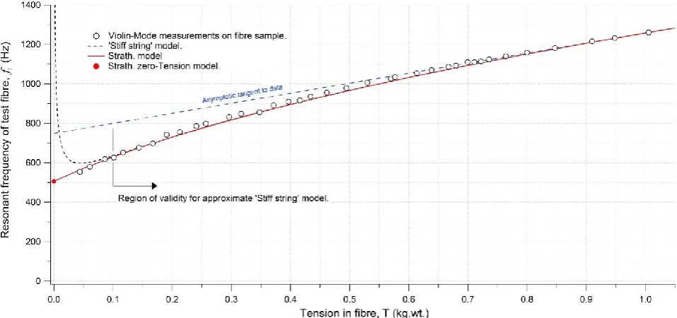
Figure 6 also shows the theory ‘Violin-Mode resonant frequency as a function of fibre tension,’ as outlined in the Appendix to this work. The full (red) line is the closed-form result for non-zero Tension, T, and the single red point is from the same theory, but for tension T = 0. In both cases, the fibre’s effective length L = 71 mm, and the density and elasticity of vitreous silica were taken to be = 2.203 103 kgm3, and E = 71.7 GPa,
respectively. The fibre’s diameter d was used as a fitting parameter, and the fit value used was d = 0.50 mm. Also shown in the Figure (by the black dashed line) is the ‘stiff string’ closed-form theory from reference [17, eqn. 16.9], this being valid for tensions T > 0.1 kg.wt. (approximately); and see also [18], which covers the full range of tension down to T = 0, albeit numerically. The fit to the data was obtained using this theory with a fibre diameter of d = 0.51 mm. Both expressions are seen to be equally good fits to the measured data, however, over their respective regions of application.
Figure 6. Resonant (Violin-Mode) frequency of the test fibre in air, measured at the AC (VM) output of the amplifier as a function of applied tension in the fibre sample, as the fibre was excited acoustically by a distant loudspeaker (open circles). The fibre’s tension was increased steadily from 43.5 grammes wt. (0.427 N) to 1.0054 kg. wt. (9.863 N). Theoretical traces: please refer to the legend in the Figure (and to the text). The dashed ‘Asymptotic tangent to data’ line is a linear fit to the data for Tension > 0.75 kg.wt.
4. Conclusions
[image:7.595.72.551.318.543.2]8 results show that our model, which used simply an ‘effective length’ for the fibre, is appropriate, here. Moreover, the theoretical resonant VM frequency of a full aLIGO fused silica suspension fibre also was calculated by means of the theory presented in the Appendix. This fibre was taken to be 600 mm long by 0.4 mm in diameter. Using, once again, values for the fibre’s density and elasticity of = 2.203 103 kgm3, and E = 71.7
GPa, respectively, yielded in this case a fundamental resonant frequency of 500.9 Hz, under a tension of 10 kg.wt.—10 kg.wt. being the nominal (and high) tension experienced by each of the aLIGO suspension fibres for the case of a 40 kg test-mass/mirror suspended by four such fibres.
On the other hand, a simple ‘vibrating stretched-wire’ calculation of the fundamental VM
frequency, 𝑓1, of such a fibre, where T = 98.1 N is the fibre’s tension (i.e., 10 kg.wt.), and is its mass per unit length (and 𝑓1 = (1 2L⁄ )√T μ⁄ ), leads to the slightly lower resonant
frequency of 496 Hz. For comparison, the fundamental VM frequencies of aLIGO suspension fibres have been measured (subsequent to this work, and independently from the interferometers) on a test suspension at MIT, where a 40 kg dummy (aluminium alloy) test mass was suspended in air [19]. In this case, the actual VM frequencies of the four suspension fibres were found to be bounded by (499.6 ± 2.3) Hz. Unfortunately, no meaningful error bars can be placed around the theoretical figure of 500.9 Hz, calculated here for such suspension fibres, because—for reasons of safety—the suspension fibres of the test-suspension could not be touched, and the values of L = 0.6 m, and d = 0.4 mm, whilst being nominally correct, could not be verified. Although the closeness of the theoretical result to the actual measured resonant frequencies might be fortuitous, it is clear, nevertheless, that even in such highly tensioned fibres, where their lengths are very much greater than their diameters, the theory presented here predicts that their internal elasticity has increased their fundamental resonant frequencies by (an easily measurable) 1%.
On the question of the instrumentation used in this work, the tension measuring system, which was developed specifically for monitoring fibre tension, performed well beyond expectations, with a linearity of (1.00000 ± 8 106) volts/kg.wt., and with an offset of
0.0785 ± 0.0184 mV (i.e., close to 0.08 grammes wt.).
At the time of writing the Violin-Mode amplifier and sensor system, which were tested here, have not been adopted for aLIGO, and, indeed, the need for separate VM sensing and damping has not yet been demonstrated. The current baseline solution is to use aLIGO’s Arm Length Stabilization system as a VM sensor / damper [20]. In fact, the issue of vacuum compatibility remains unresolved for the VM sensor employed in this work, because the Hamamatsu photodiodes used for the detector elements had been encapsulated, using an unknown epoxy. However, were it to become necessary, the issue of the epoxy for the photodiodes from this, or another, manufacturer probably could be resolved, and the LEDs and other components used are likely to prove vacuum compliant, or have vacuum-compliant alternatives.
5. Acknowledgements
9 profoundly indebted, and NAL and KVT are grateful for the support of grant STFC PP/F00110X/1, which sustained this work on the Violin-Mode detection system.
References
[1] Harry G M (for the LIGO Scientific Collaboration) 2010 Advanced LIGO: the next generation of gravitational wave detectors. Class. Quantum Grav.27 084006
(12pp).
[2] Abbott B P et al 2009 LIGO: The Laser Interferometer Gravitational-Wave Observatory Rep. Prog. Phys.72 1–25.
[3] Raab F J et al 2004 Overview of LIGO Instrumentation Proceedings of SPIE5500
11–24 (29 Sept.).
[4] Aston S M et al 2012 Update on quadruple suspension design for Advanced LIGO Class. Quantum Grav.29 235004 (25pp).
[5] Heptonstall A et al 2011 Invited Article: CO2 laser production of fused silica fibers
for use in interferometric gravitational wave detector mirror suspensions Rev. Sci. Instrum.82 011301 1–9.
[6] Cumming A V et al 2012 Design and development of the advanced LIGO monolithic fused silica suspension Class. Quantum Grav.29 035003 (18pp). [7] Carbone, L., et al. 2012 Sensors and actuators for the Advanced LIGO mirror
suspensions. Class. Quantum Gravi.29 11 115005 (14pp).
[8] Tokmakov K.V. , et al 2012 A study of the fracture mechanisms in pristine silica fibres utilising high speed imaging techniques, Journal of Non-Crystalline Solids
358, 14, 1699 doi:10.1016/j.jnoncrysol.2012.05.005.
[9] Lockerbie N A and Tokmakov K V 2014 A ‘Violin-Mode’ shadow sensor for interferometric gravitational wave detectors Meas. Sci. Technol. 25, 12, 12p., 125110; http://dx.doi.org/10.1088/0957-0233/25/12/125110.
[10] Lockerbie N A and Tokmakov K V and Strain K A 2014 A source of illumination for low-noise ‘Violin-Mode’ shadow sensors, intended for use in interferometric gravitational wave detectors Meas. Sci. Technol. 25,12, 12 p., 125111;
http://dx.doi.org/10.1088/0957-0233/25/12/125111.
[11] Lockerbie, N.A. and Tokmakov, K.V. A step-wise steerable source of illumination for low-noise ‘Violin-Mode’ shadow sensors, intended for use in interferometric gravitational wave detectors LIGO Document No. P1500195-v2, available at
https://dcc.ligo.org/.
[12] Gonzalez G. I., and Saulson P.R. 1994 Brownian motion of a mass suspended by an anelastic wire J. Acoust. Soc. Am.96 (1), July 1994.
[13] Dmitriev A et al 2010 Controlled damping of high-Q violin modes in fused silica suspension fibers. Class. Quantum Grav.27 025009 (8pp).
[14] Lockerbie, N.A. and Tokmakov, K.V. 2014. A low-noise transimpedance amplifier for the detection of “Violin-Mode” resonances in advanced Laser
Interferometer Gravitational wave Observatory suspensions. Rev. Sci. Instrum. 85, 114705; http://dx.doi.org/10.1063/1.4900955.
[15] Lockerbie, N.A. and Tokmakov, K.V. An AC modulated Near InfraRed gain calibration system for a Violin-Mode transimpedance amplifier, intended for advanced LIGO LIGO Document No. P1500199-v2 available at https://dcc.ligo.org/.
[16] Lockerbie, N.A. and Tokmakov, K.V. 2014. Quasi-static displacement calibration system for a “Violin-Mode” shadow-sensor intended for Gravitational Wave
detector suspensions. Rev. Sci. Instrum. 85, 105003 (2014);
10 [17] “Vibration and Sound,” Philip M. Morse, McGraw Hill, 1936 (ISBN-10: 0883182874
—paperback, 1991).
[18] Bokaian, A. 1990 Natural Frequencies of Beams under Tensile Axial Loads, Journal of Sound and Vibration, 142 3 481–498.
[19] Lockerbie, N.A., Carbone , L., Shapiro, B., Tokmakov, K.V., Bell, A., and Strain, K.A. 2011. First results from the ‘Violin-Mode’ tests on an advanced LIGO suspension at MIT. Class. Quantum Grav. 245001 (12pp)
http://iopscience.iop.org/0264-9381/28/24/245001.
[20] Instrument Science White Paper 2012 LIGO-T1200199-v2, p71https://dcc.ligo.org/. [21] “An Introduction to the Properties of Condensed Matter,” D. J. Barber, and
R. Loudon, Cambridge University Press, 1989 (ISBN 0 521 26277 1), equations2.150, and 2.160.
[22] “The Calculus of Variations,” Bruce van Brunt, Springer, 2006 (ISBN 0 387 40247 0), pp 135–143.
Appendix: Theory of Violin-Mode resonant frequency as a function of fibre tension
Figure 7: Deflection of a silica fibre, of length L, as it is loaded by a uniform (along the x-axis, and in the y-direction) transverse acceleration, a.
In Figure 7 a vertically-orientated silica fibre, of length L, is clamped at both ends (x =±L/2),
whilst being under a tension, T. Here, the fibre experiences a static uniform transverse acceleration, a, causing it to bow- out in the negative-y direction, as indicated. The (negative) potential energy of the fibre due to this acceleration can be written
P.E.accel. =
/2
/2 μ .a y dx
LL , (1)
where is the mass per unit length of the fibre, and y its deflection. The curved fibre also stores (positive) elastic energy, such that
P.E.elast. =
/2 2
1 2
/2 y dx
L EIL , (2)
where yis the curvature of the fibre, E is its elasticity, and I is its area moment of inertia about its neutral bending plane [21].
I d4/64 for a fibre of circular
cross-section, and diameter = d.
In addition, the transverse deformation y(x) of the fibre causes its length to be slightly greater
than its un-deformed value, L, and this stretching of the fibre takes place against the tension force, T. Thus, a (positive ) tensional energy equal to
P.E.tension =
/2 1 2
2
/2 y dx
L TL (3)
is stored in the tensioned fibre. The total P.E. of the system is therefore (from eqns. 1–3)
P.E.Total =
/2 2 2
1
2
/2 2μ .a y y y dxL
L EI T , where
,
1,
.1
y x y x L
x
y d (4)
The optimal shape y(x) of the fibre is that which minimizes P.E.Total, and this can be found
using the Calculus of Variations [22], via the Euler-Poisson (E-P) equation—which is used where there are derivatives of order higher than the first (as here). The E-P is
1 0... 2 2
y y yn
[image:10.595.93.278.303.544.2]11 where Fy denotes partial differentiation of the integrand F of equation 4 with respect to y, etc.
Applying the E-P equation to this integrand yields
0μ 2 2 y dx d y dx d
a T EI , which, upon rearranging, leads to
4 μ 0
EI EI T a y
y . (5) Upon solving equation 5—for the particular case of T = 0—and by applying clamped-clamped boundary conditions to the fibre’s ends (x = ±L/2: y = 0, y= 0), along with the symmetry condition (y= 0) at x = 0 (the centre of the fibre), the profile of the fibre can be found to be
EI 384 4 μ 2 2 2 x a xy L (T = 0). (6) Parenthetically, if y(x) is substituted back into equation 1—and (after differentiation with respect to x twice, and once, as appropriate), into equations 2 and 3—it can be shown that P.E.accel. ≡ 2 (P.E.elast. + P.E.tension), or, P.E.Total ≡ (P.E.elast. + P.E.tension). In the case of
equation 6, P.E.tension = 0, of course, since T =0; but P.E.Total ≡ (P.E.elast. + P.E.tension)
remains true even when T ≠ 0, P.E.tension≠ 0, and y(x) is given by equation 9, below.
Rayleigh’s method for finding theoretically (e.g.) a fibre’s natural resonant frequencies is particularly appropriate to finding the fundamental frequency. It relies upon the complete conversion of potential into kinetic energy, and vice versa, in an oscillating conservative system. For example: if, under a uniform transverse acceleration, a, the fibre were to take up a static deflection, y(x); and if the fibre then were to be released (a = 0), so that subsequently it oscillated symmetrically back-and-forth at its natural resonant angular frequency, ω1, about its un-deflected shape: then, with all parts of the fibre moving in phase at this frequency, the time-dependent deflection of the fibre could be written 𝑦(𝑥, 𝑡) = 𝑦(𝑥)cos (ω1𝑡), (say).
Thus, the fibre will be at rest, periodically, with a deflection of ±y(x)—and with all of its energy stored as P.E. Conversely, at some point in time the fibre will have no deflection (i.e., y(x,t) = 0, x), but it will have, instead, a maximum transverse velocity 𝑣Max(𝑥), given
by 𝑣Max(𝑥) ≡𝑦̇(𝑥, 𝑡)|Max= ω1|𝑦(𝑥)|. Consequently, in this case the stored P.E. will be zero,
whilst, the kinetic energy per length 𝑑𝑥 of the fibre will be 12𝑚𝑣Max2 (𝑥)
,
where 𝑚 = μ 𝑑𝑥 ( isthe mass per unit length of the fibre). Therefore, for the full fibre, the maximum K.E. will be K.E.Max y
x dxL L
/2
2 / 2 2 1 2 ω μ
. (7) By equating this energy to (P.E.elast. + P.E.tension), i.e., to the total stored energy of the fibre at
rest, e.g., ‘on release,’ the frequency of vibration for that particular y(x) can be found. This frequency (ω1) is necessarily independent of the static driving amplitude, a, because a2 is a
common factor in the expressions for both the K.E. and the stored P.E. In this way, Rayleigh’s method leads to a fundamental resonant Violin-Mode frequency for the fibre of
𝑓1
=
3√14 𝜋L2 √EI
μ [Hz], (for T = 0), where ω1 = 2𝜋𝑓1. (8)
This frequency is marked by the single data point labelled ‘Strath. zero-Tension model’, in Figure 6. The numerical prefactor of 3√14 𝜋⁄ in equation 8 evaluates to 3.573. In comparison, an analysis of the fundamental frequency of a vibrating elastic bar [17, equation 15.11], gives an equation for 𝑓1with the same dependencies as equation (8), and with an almost identical
numerical prefactor, as well (although expressed differently)—of 3.561, in that case.
12
, 2 coth 4 4 1 1 2μ 2 2
EI T EI T T EI
T EIT
EI EI L L L L L x e e e a x
y (9)
where (−L2≤ 𝑥 ≤L2), and (T > 103 kg.wt.)—the inequality must hold, in practice, for
numerical stability. Ostensibly, y(x) calculated using equation 9, withT→ 0, bears no relation to that given by equation 6; but, in fact, they are practically indistinguishable. Once again, equating K.E.Max, from equation 7, with the total stored energy on ‘release’ (≡P.E.accel./2)—
the energies being calculated now using equation 9—allows the fundamental resonant Violin-Mode frequency to be found. This approach actually led to a closed-form solution for ω1(= 2𝜋𝑓1), but the consequential expression is too large to be included here. However, the
resulting values of 𝑓1have been plotted as a function of T (in kg.wt) in Figure 6, using this

![Figure 7: Deflection of a silica fibre, of length about its neutral bending plane [21]](https://thumb-us.123doks.com/thumbv2/123dok_us/1538680.106435/10.595.93.278.303.544/figure-deflection-silica-fibre-length-neutral-bending-plane.webp)