End-user feature labeling: Supervised and semi-supervised approaches based on locally-weighted logistic regression

City, University of London Institutional Repository

Citation

:

10.1016/j.artint.2013.08.003

This is the unspecified version of the paper.

This version of the publication may differ from the final published

version.

Permanent repository link:

Link to published version

:

Copyright and reuse:

City Research Online aims to make research

outputs of City, University of London available to a wider audience.

Copyright and Moral Rights remain with the author(s) and/or copyright

holders. URLs from City Research Online may be freely distributed and

linked to.

Supervised and Semi-supervised Approaches Based on

Locally-Weighted Logistic Regression

Shubhomoy Das

, Travis Moore

, Weng-Keen Wong

,

Simone Stumpf

, Ian Oberst

, Kevin McIntosh

, Margaret Burnett

†

Oregon State University, OR, USA

‡

City University London, UK

__________________________________________________________________________________

Abstract

When intelligent interfaces, such as intelligent desktop assistants, email classifiers, and recommender systems, customize themselves to a particular end user, such customizations can decrease productivity and increase frustration due to inaccurate predictions—especially in early stages when training data is limited. The end user can improve the learning algorithm by tediously labeling a substantial amount of additional training data, but this takes time and is too ad hoc to target a particular area of inaccuracy. To solve this problem, we propose new supervised and semi-supervised learning algorithms based on locally weighted logistic regression for feature labeling by

end users, enabling them to point out which features are important for a class, rather than provide new training instances.

We first evaluate our algorithms against other feature labeling algorithms under idealized conditions using feature labels generated by an oracle. In addition, another of our contributions is an evaluation of feature labeling algorithms under real world conditions using feature labels harvested from actual end users in our user study. Our user study is the first statistical user study for feature labeling involving a large number of end users (43 participants), all of whom have no background in machine learning.

Our supervised and semi-supervised algorithms were among the best performers when compared to other feature labeling algorithms in the idealized setting and they are also robust to poor quality feature labels provided by ordinary end users in our study. We also perform an analysis to investigate the relative gains of incorporating the different sources of knowledge available in the labeled training set, the feature labels and the unlabeled data. Together, our results strongly suggest that feature labeling by end users is both viable and effective for allowing end users to improve the learning algorithm behind their customized applications.

* Corresponding author

E-mail address: [email protected] (Shubhomoy Das, 1148 Kelley Engineering Center, Corvallis, OR 97331-5501, USA, Ph: 1-541-908-6949).

1

© 2012 Elsevier B.V. All rights reserved.

Keywords: Feature labeling, locally weighted logistic regression, machine learning, intelligent interfaces, semi-supervised learning

__________________________________________________________________________________________

1 Introduction

Many applications, powered by machine learning, customize themselves to a particular end user’s preferences. Such applications include email classifiers, recommender systems, intelligent desktop assistants, and other intelligent user interfaces. To accomplish this customization, the application must learn from the particular end user—which obviously cannot happen until after the system is deployed and training data from that specific end user is obtained.

Customizing to the end user’s preferences is challenging, especially when there is limited training data, such as when the application is first deployed. The end user could select additional training instances to label, or the learning algorithm could ask the user to provide class labels for strategically chosen instances that would most inform the learning algorithm, as is done in traditional active learning [7, 31]. Labeling instances, however, has its drawbacks. First, labeling data instances is a tedious process and a substantial number of instances must often be labeled before a change to the learning algorithm is noticeable to an end user. Second, in a streaming data setting, such as news filtering or email classification, active learning is not applicable as the system has no control over which data instance arrives next. Finally, if a rare group of instances is incorrectly classified, the learning algorithm cannot be “corrected” until the user labels instances with this rare combination of attributes. Since this group is rare, the cost, in terms of time or effort, to acquire such data instances could be very expensive [1].

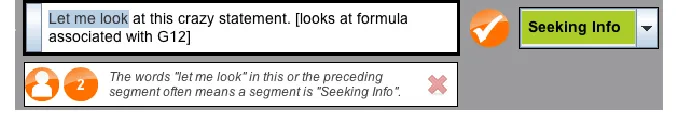
To overcome these problems, in this paper we investigate the possibility of end-user feature labeling [29, 10, 33, 1], namely allowing end users to label features instead of instances. Here, the term feature refers to an attribute of a data instance that is useful for predicting the class label; for example, rather than labeling entire documents, an end user could point out which words (features) in the document are most indicative of certain class labels. Figure 1 shows this approach in our formative research’s user interface [15], which allowed HCI

researchers to point out words that were predictive of that transcript segment’s label. Raghavan et al. [28, 29] found that labeling a feature took humans roughly a fifth of the time as a document and the benefits of feature labeling were greatest when the training set sizes were small. However, their work did not evaluate feature labeling in a statistical user study involving a large number of actual end users.

Allowing end users, who are not likely to be educated in machine learning, to use feature labeling introduces new challenges to learning algorithms. End users’ choices of features may be noisy, inconsistent, and might vary greatly in ability to improve the predictive power of the machine learning algorithm. This paper therefore investigates algorithms able to stand up to these challenges.

Our research contributions are as follows. First, we present a new supervised learning algorithm for taking end-user feature labels into account, based on Locally Weighted Logistic Regression. In order to evaluate our feature labeling algorithm, we perform an empirical comparison on multiple data sets under ideal conditions, using feature labels obtained from an oracle, and under real-world conditions for one particular dataset, using feature labels harvested from actual end users. For the latter study, we present a user study in which ordinary end users, unfamiliar with machine learning, chose the feature labels themselves— with no restrictions as to what they could select as features. Our algorithm was among the best performing feature labeling algorithms in the idealized setting and it was also robust to poor quality feature labels provided by ordinary end users in our study.

Next, we present a semi-supervised version of our feature labeling algorithm which assumes that an unlabeled set of instances is present during training. The semi-supervised setting for feature labeling incorporates knowledge from three sources: a small labeled training set, the feature labels provided by the end user and information from the implicit structure of the unlabeled data. We evaluate our semi-supervised algorithm using both oracle feature labels and end-user feature labels from the user study mentioned above. Our feature labeling algorithm is one of the best performing algorithms with oracle feature labels and the best performer with lower quality feature labels from end users. With our results, we can compare the relative gains using the different sources of knowledge available in the training set, the feature labels, and the unlabeled data. Our analysis shows that incorporating unlabeled data during learning sometimes produces worse performance than just using a purely supervised learning approach, both with and without feature labeling. However, adding the information from feature labels consistently improves performance over not including this information, both in the supervised and semi-supervised settings.

2 Related Work

We divide the approaches for feature labeling into supervised and semi-supervised feature labeling algorithms. Supervised feature labeling algorithms require only a training set of labeled instances. On the other hand, semi-supervised feature labeling requires both a labeled training set as well as a pool of unlabeled data, which is assumed to be relatively easy to obtain.

Two of the SVM-based methods presented by Raghavan and Allen [29] involved supervised feature labeling. Their Method 1 scaled features indicated as relevant by the user by a constant a and the rest of the features by a constant d

(where a ≥ d). In Method 2, the user indicated that the jth feature was relevant for a class label l. For each feature-label pair, Method 2 created a pseudo-document consisting of a value r in index j, zeroes elsewhere and a class label of l. The r

parameter controlled the influence of the support vectors of the pseudo-documents on the separating hyperplane.

Another group of supervised feature labeling algorithms were based on multinomial naïve Bayes. The pooling multinomials approach [25] combined parameters from a multinomial naïve Bayes trained on labeled instances and another derived from background knowledge, which in this case were feature labels. This approach, however, was restricted to Boolean class labels. Settles [32] proposed another method based on naïve Bayes in which he changed the priors for labeled features. If a feature was labeled with a class, the corresponding parameter was given a Dirichlet prior of ( ), where was a tunable parameter, while all unlabeled features were given a uniform Dirichlet prior of 1.

The majority of the work in feature labeling took a semi-supervised approach. A common strategy employed by several methods was to use the user feedback to label the unlabeled data and then incorporate these soft labels into training. Method 3 of [29], following the approach of [38], associated slack variables with the soft labeled data to influence the position of the margin for an SVM. The user co-training algorithm of Stumpf et al. [35] treated the user’s feature labels like a classifier and combined it in the co-training framework [4] with naïve Bayes. The MNB approach by Settles could be extended to a semi-supervised approach by soft-labeling the unlabeled data and then re-estimating the MNB parameters [11]. Finally, the approach by Liu et al. [20] modified the EM algorithm to incorporate labels produced by “representative words” for each class selected by the user.

problems as diverse as multi-view learning [11] and transfer learning [22]. Examples of these approaches include Constraint Driven Learning [5], Generalized Expectation [22, 10], Learning with Measurements [19] and Posterior Regularization [12, 11]. Ganchev et al. [11] described the relationships between these approaches and the subtle differences in the approximations these algorithms employed for inference.

We briefly describe Generalized Expectation (GE) in more detail since it was specifically applied to feature labeling [10] and we will be using it in our experiments. GE is a framework for incorporating preferences about variable expectations during parameter estimation. We can describe GE as trying to maximize a score function S between a model’s expectation of and a target

value ̃, as shown below:

[ ] ̃

For instance, in Maximum Likelihood Estimation, the score function is the negative cross entropy and the target value is the empirical distribution on the training data. We can fit our algorithm into the GE framework by using the empirical distribution as the target value and a weighted negative cross entropy as the score function. Our approach is very different from prior work with GE which incorporates feature labels by changing the target value, rather than our approach of changing the score function.

Aside from supervised and semi-supervised feature labeling, other work in feature labeling investigated dual supervision [33], which is a term used to describe the process of labeling both instances and features. Raghavan and Allen [29] combined feature labeling with uncertainty sampling for instance labeling in their tandem learning approach. Other dual supervision approaches include a graph-based transduction algorithm [33] and an approach using pooled multinomials [2]. The focus of these last two papers was on active learning for dual supervision, which chose instances and features for labeling. Our work differs in that it is the end users, not the active learning algorithm, that choose the features for labeling. Furthermore, we are investigating the effects of labeling only features, not instances, especially with an eye to the initial training period when training data is limited.

All of the above methods dealt with labeling existing features. Roth and Small [30] allowed users to create new features by replacing features corresponding to semantically related words with a Semantically Related Word List (SWRL) feature. Their focus, however, was on creating SWRLs to improve classifiers rather than feature labeling. In our user study, we allow end users to construct new features and label them.

Finally, most of the prior work in feature labeling evaluated algorithms under ideal conditions, such as feature labels obtained from an oracle [2, 33]. Some prior work [28, 32] has evaluated feature labeling algorithms using both oracle feature labels and labels obtained from user experiments. However, these experiments were on a small scale with only a handful of users and a subset of these users were knowledgeable about machine learning. In contrast, we perform a large scale statistical study involving 43 participants, all of whom have no background in machine learning or human computer interaction. These non-expert end-users can introduce noisy and inconsistent feature labels. Our study investigates both the use of ideal oracle feature labels and feature labels provided by real world end users.

3 Theory / Calculation

Our approach, which we call LWLR-FL, incorporates feature labeling into Locally Weighted Logistic Regression (LWLR). LWLR-SS-FL then extends FL further for semi-supervised learning. To provide context for LWLR-FL, we first describe (global) Logistic Regression and LWLR.

3.1 Background

Logistic Regression (LR) [13] is a well-known method in statistics for predicting a discrete class label yi given a data instance xi=(xi

1_,…,x i

D

) with D

features; we refer to the dth feature, without reference to a specific data instance, using the superscript notation i.e. xd. LR models the conditional probability

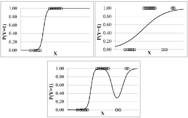
P(yi|xi) by fitting a logistic function to the training data. Figure 2 (left) illustrates

the s-shaped logistic function fit to training data from two classes (squares and circles). Notice that the data is perfectly separable, in the sense that data to the left of the bend in the “S” is classified as a square and data to the right as a circle.

The conditional probability for an M-class problem is:

( ) ( ∑ )

In the equation above, the notation cj refers to the jth class. The parameters 

= (1, …, M) are computed by maximizing the conditional log likelihood, which

cannot be solved in closed form but must be done numerically.

LR assumes that the parameters  are the same across all data points. Although this approach works reasonably well when the classes are linearly separable, it fails when the actual decision boundaries are more complex and when the data is noisy [9], which is often the case with real-world data. For instance, Figure 2 (top right) illustrates a problematic case for LR when the data is not cleanly separable by the logistic function. Here, the s-shaped logistic function fits the data poorly, resulting in the two squares on the right to be classified as circles.

One solution for dealing with the difficult case in Figure 2 is to use Locally Weighted Logistic Regression (LWLR) [6, 9], in which the logistic function is fit locally to a small neighborhood around a query point xq to be classified. Figure 2

(bottom) illustrates LWLR fit to the data points. Intuitively, LWLR gives more weight to training points that are “closer” to the query point than those farther away. A common function used to determine the closeness of text documents is cosine similarity. Since we want the distance to increase when a training instance

Fig. 2. (top left) The Logistic Function fit to two classes: squares (y=0) and circles (y=1). (top right) A non-separable case where (global) Logistic Regression will have difficulty separating the circle class (y=1) from the square class (y=0), resulting in a poor fit. Note that the square data points to

the right will be classified as circles. (bottom) A non-separable case where Locally Weighted Logistic Regression will be effective in separating the

xi is less similar to the query instance xq, we use cosim(xq,xi) = 1 – cos(xq,xi) as

the baseline distance function for LWLR. In Section 3.2, we will describe how we extend this reweighting of training instances to perform feature labeling.

The log-likelihood of data in LWLR is computed with respect to the query instance xq as

∑ ( ) ( ) (1)

where,

( ) ( ( ) ) (2)

The weight w(xq, xi) is a kernel function which decays with the distance f(xq, xi).

The parameter k is the kernel width, which smoothes out more noise as the value of k increases. As a consequence of having to fit the logistic function locally to a query point, LWLR is considered a lazy algorithm and we now need to train the classifier each time it receives a query point. However, in many cases, we gain a much higher accuracy with this tradeoff in efficiency.

Maximizing lw() with respect to the parameters  cannot be done in closed

form. In our experiments, we solve it using L-BFGS [26] for which we need to compute the partial derivative of lw() with respect to the  parameters. The

partial derivative below computes the gradient for the log-likelihood. In the formula below, the expression [yi =cj] takes the value of 1 if the expression in the

brackets is true, and 0 otherwise.

∑ ( ) ( [ ]

( ∑

))

(3) where,

∑ ( ∑

)

3.2 Adding Feature Labeling to Locally Weighted Logistic Regression (LWLR-FL)

weight training instances differently, rather than its ability to handle non-linear decision boundaries. Intuitively, we use feature labels provided by the end user to define the local neighborhood surrounding the query point. Training instances that are more similar to the query point according to the feature label information are considered to be closer and hence assigned higher weight. We modify the baseline cosim(xq, xi) distance function to incorporate feature labels. Our

modified distance function between xq and xi has two distinct components – one

based only on their features (satisfied by the baseline distance cosim(xq, xi)), and

the other based on class labels. Since xq does not have an associated class label,

we use the class label of xi and the feature label information for computing the

label similarity.

The label similarity between xq and xi is based on the difference between the

class-relevant and class-irrelevant feature contributions. A class-relevant feature is a feature that is labeled with the class label yi of instance xi as specified by the

feature labels. The class-relevant feature contribution is the sum of the values of all class-relevant features in xq, where xq is represented as an L2-normalized

TFIDF vector. Similarly, a class-irrelevant feature is a feature that is labeled with a class label other thanyi. The class-irrelevant feature contribution refers to

the sum of values of all class-irrelevant features in xq.

We now define the user feature label matrix R as:

[ ] [

]

where rj(x d

) = 1 if the dth feature is labeled to be important for class label cj and 0

otherwise. We will denote the jth column of R by R(j). Let U be a (D × 1)

column vector in which the ith entry is 1 if the ith feature has been marked important in any class. All other entries are zero.

On the basis of the above definitions, the difference between the class-relevant and class-irclass-relevant feature weights is computed as:

(( )

)

The term R(yi)

T

xq is sum of class-relevant feature values for class yi and (U –

R(yi))

T

xq is the sum of class-irrelevant feature values. Since we have (M-1) class

labels excluding yi, we divide the class-irrelevant feature contributions by (M – 1)

to appropriately balance the difference.

(( )

)

The complete distance function now becomes:

( ) ( ) [ (( )

)]

The above function could turn out negative in some cases. Hence, we introduce a max term in the weight computation to handle this scenario.

( ) ( ( ( )) ) (4)

Putting these pieces together, we now have a distance function that incorporates the feature labels into LWLR.

Since LWLR-FL and LWLR are lazy algorithms, meaning that they do not perform training until a query is made, each query has a computational complexity of O(n), where n is the number of instances in the training set. Although the computational cost can be expensive with a large training set, the LWLR-FL algorithm is intended to be applied to small training sets during the initial period when a learning algorithm is first deployed. With small training sets, such as those in our experiments, each query only takes milliseconds on a standard desktop computer, making the LWLR-FL algorithm viable in an interactive setting.

3.3 Extending LWLR-FL to Semi-supervised Learning

The notion of locality around an unlabeled query instance xq (in LWLR and

LWLR-FL) has so far been based on a similarity measure between only labeled instances and xq. We now extend the similarity measure to include information

from other unlabeled instances as well using label diffusion [39, 41]. We refer to our semi-supervised algorithm which uses no feature labeling information as LWLR-SS and the one using feature labeling information as LWLR-SS-FL.

until a stationary state is reached. At this stationary state we have at a pairwise similarity matrix which takes into account the distance the labels had to diffuse through rather than just the Euclidean distances.

Let be the set of unlabeled instances, be the set of labeled instances, and be the total number of instances (| ). Let _{[ ]} be an initial affinity matrix, prior to label diffusion, that captures the similarity between two data instances. When , otherwise for , LWLR-SS uses the

following similarity measure between any two instances xi and xj:

(

).

Define [ ] as a diagonal matrix where ∑ and let _{. The matrix}

[ ] will contain all pairwise

similarities when label diffusion reaches the stationary state. Here the parameter controls the rate of label propagation and _{[ ]} is an identity matrix. We can consider as being the distance matrix defined within a transformed space (referred to as the manifold space.)

The likelihood function for the query instance xq for LWLR-SS is now

modified to be ∑ ( ) where we have replaced

( ) by in Eq. (1) and Eq. (3).

The LWLR-SS-FL algorithm incorporates feature labeling into LWLR-SS by using the following similarity measure:

̂

{

( ( ( )) )

( )

Apart from this modification to the similarity measure, the LWLR-SS-FL algorithm is identical to the LWLR-SS algorithm.

The algorithm for the semi-supervised learning can be summarized in the following steps.

Algorithm 3.1: Semi-supervised LWLR-FL (LWLR-SS-FL) 1. Setup matrices ̂ as defined above.

2. Compute

3. Normalize all values of into range [0,1] by dividing row by the diagonal element . Since the diagonal elements are self-similarities,

4. For each unlabeled instance , train a locally weighted logistic regression classifier with instance weights set to normalized , where

and classify .

4 Material and Methods

To evaluate the LWLR-FL and LWLR-SS-FL algorithms, we applied them to six real-world text data sets, with two kinds of studies. First, to avoid the prohibitive expense of performing a separate user study on each data set, we followed the usual machine learning convention [29, 33], and simulated end-user feature labeling on multiple data sets using a feature label oracle. Second, we then performed a study with real users on one particular data set to investigate the effectiveness of using feature labels from end users.

4.1 Oracle Study

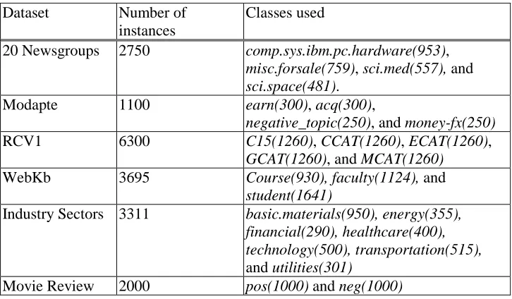
In our oracle-based experiments, we used six common text classification datasets: 20 Newsgroups [16], the Modapte split of the Reuters dataset [17], the Reuters Corpus Volume 1 (RCV1) dataset [18], WebKb [8], the Industry Sector dataset [24], and the Movie Review dataset [27]. As a pre-processing step, the text documents were converted into TF-IDF representation then L2-normalized. We used a vocabulary consisting of unigrams with stopwords removed.

Dataset Number of instances

Classes used

20 Newsgroups 2750 comp.sys.ibm.pc.hardware(953),

misc.forsale(759), sci.med(557), and

sci.space(481). Modapte 1100 earn(300), acq(300),

negative_topic(250), and money-fx(250)

RCV1 6300 C15(1260), CCAT(1260), ECAT(1260),

GCAT(1260), and MCAT(1260)

WebKb 3695 Course(930), faculty(1124), and

student(1641)

Industry Sectors 3311 basic.materials(950), energy(355), financial(290), healthcare(400), technology(500), transportation(515),

and utilities(301)

Movie Review 2000 pos(1000) and neg(1000)

Table 1 summarizes the number of instances and the classes used from each of these datasets. Class imbalance, however, can be a problem in some of these datasets. For instance, in WebKb, the smallest class is approximately 1/16th the size of the largest class. In order to avoid class imbalance issues, we chose the largest classes with roughly the same number of data instances in each class and avoided classes with an extremely small number of data instances.

For 20 Newsgroups, we chose four classes of newsgroups that end users in our user study could understand easily without the need for specialized knowledge. Since we would also present articles from these newsgroups to end users in our user study (Section 4.2), we wanted to preserve the topical coherence of articles by choosing articles that fell within a relatively short date range that included a large number of articles from these newsgroups. As a result, we chose 2750 articles from these four newsgroups within the date range April 1, 1993-April 23, 1993.

4.1.1 Oracle Study: Supervised Learning

We compared LWLR-FL against three SVM-based algorithms from [29], which are competitive supervised feature labeling methods. Specifically, these SVM-based algorithms are Method 1, Method 2 and a combination of both Methods 1 and 2. We abbreviate these variants as SVM-M1, SVM-M2, and SVM-M1M2 respectively. For these SVM-based methods, we tried linear, RBF and polynomial kernels and found the linear kernel to give the best accuracy. As a result, we only report SVM results with linear kernels.

In addition, we compared LWLR-FL against the Multinomial Naïve Bayes algorithm from [32]. Since all but one of the datasets used in our experiments were multi-class, we did not evaluate against the pooling multinomials approach [25] which was specifically for binary class data. We refer to the MNB-based algorithm as MNB/Priors.

Since we were interested in the benefits due solely to feature labeling, we did not compare against methods such as Tandem Learning [29] and dual supervision [2, 33] which allow users to label both features and data instances after the algorithm has been trained. Other techniques for feature labeling are semi-supervised methods, which leverage information from a pool of unlabeled data in addition to the information in feature labels. We will compare the semi-supervised version of LWLR-FL against semi-semi-supervised methods in Section 4.1.2.

one oracle feature label per class, two oracle feature labels per class, and so on until a total of ten per class were added. These oracle feature labels were added in the order of highest information gain. Therefore the oracle study provides an optimistic estimate on the potential gains of using these feature labeling algorithms by providing enough ideal feature labels to benefit the algorithm and by carefully tuning the parameters of the feature labeling algorithms over a large validation set.

Each dataset was split into training, validation and testing sets. Since past work [29] has shown that feature labeling is most effective when the training set sizes are small, we created training sets consisting of six instances per class. Most of our experiments dealt with a multiclass classification problem with between four and seven classes (rather than binary classification as in [29]), so the total training set sizes at six per class were 24 for 20 Newsgroups, 24 for the Modapte split, 30 for RCV1, 42 for Industry Sectors, 18 for WebKb, and 12 for the binary Movie Review dataset. The training set consisted of an equal number of data instances from each class in order to avoid biases due to class imbalance. The validation set, which was used to tune algorithm parameters, was composed of 100 data points for all datasets. All validation set were equally distributed among all the classes. For all datasets, we created 30 different random splits for training, validation and testing. The results were averaged over these 30 splits.

4.1.2 Oracle Study: Semi-supervised Learning

In order to evaluate the semi-supervised learning algorithms, which assume a pool of unlabeled data instances is available during training, we used the same 6 datasets as those used for supervised learning as well as the same oracle feature labels. Furthermore, we used the same training/validation/test splits, but unlike in supervised learning, we made the unlabeled data instances from the test set available during training. We used the same oracle feature labels from the previous section and present results when 10 oracle feature labels per class were provided to the semi-supervised algorithms.

We compared LWLR-SS-FL against SVM-M3, GE, and MNB/Priors+EM, which are representative algorithms from the two general strategies used for semi-supervised feature labeling. For the SVM-based methods, we experimented with different combinations of Method 1 and Method 2 with Method 3, but found that SVM-M3 worked the best. To avoid clutter, our results only show the results from SVM-M3. We chose GE because it was specifically used for feature labeling in [10] and because the GE code was readily available in the Mallet package [23]. GE has also been shown to perform better empirically than other algorithms (eg. learning with measurements) with small training data sets [19], which was our particular problem setting.

expense of tuning LWLR-SS-FL, but set √ for all datasets. This value was determined empirically and was found to give good results. The number of nearest neighbors was fixed to 100 for all datasets.

We used GE with Schapire distributions as in Druck et al. [10] where the majority class was assigned a weight 0.9. The Gaussian prior in GE was tuned within the range of values from 0.2 to 1.0 at steps of 0.2 using the validation set. The GE objective function can be modified to weight the GE term and the likelihood of the data in order to balance the effects of feature labels with training data. Since the training sets in our experiments were very small, the likelihood term had neglible effect and we found that using only the GE term produced the best results.

For all SVM methods, including SVM-M3, the parameters C, a, and r were tuned using a validation set. The parameter d was fixed to 1.0. For MNB/Prior and MNB/Prior+EM we tuned the prior α using the validation set. We also tuned the soft-labeling weight for unlabeled instances in MNB/Prior+EM using the validation set.

4.2 User Study

The strength of oracle studies is the ability to evaluate a variety of data sets, but their weakness is that they may not be realistic as to the choices real users might make. Therefore, for our second experiment, we conducted a user study to harvest feature labels from actual end users on the same 20 Newsgroups classes as used in Section 4.1. We then used the end users’ data to compare the performance of the same algorithms as in our oracle study, but with smaller validation sets of size 24 (six instances for each class) to simulate a realistic scenario in which end users were able to label only a limited amount of training instances for both a training and a validation set.

A starting point for our experiment’s design was the user study by Raghavan et al. [28]. However, an important difference was that we chose to remove constraints on features end users were allowed to pick. Specifically, rather than having end users select features from a pre-computed list, we allowed them to identify features by freely highlighting text directly in the documents. This gave our participants complete freedom to choose any features that they thought were predictive. Consequently, not only were these end users allowed to select existing features in the algorithm’s representation, but also to create and label new features, such as through combinations of words or punctuation.

4.2.1 Participants and Procedures

background in machine learning or human computer interaction were not allowed to participate.

Participants attended the study in parallel, with up to five participants to a session. At the start of a session, we familiarized the participants with the application to create feature labels, described in Section 4.2.2, through a brief, hands-on tutorial and self-directed exploration. All participants used the same document set during the tutorial, which was different from the main task data set (the training set). After the session they filled out a post session questionnaire asking their thoughts and suggestions for the interface, for our later use in follow-up research.

For the main experiment, the application displayed 24 previously labeled documents in four topics: Computers, Things For Sale, Medicine, and Outer Space (corresponding to the four newsgroups comp.sys.ibm.pc.hardware,

misc.forsale, sci.med, and sci.space, respectively). Each of the four topics had six documents assigned to it, which were randomly selected from a pool of 200 training instances. The order of the documents was randomized for each participant. Participants were asked to teach the machine “suggestions” by identifying features that they believed would help it label future documents. Within a time limit of twelve minutes, participants were asked to provide at least two suggestions per topic, with an emphasis placed on selecting the best features for each newsgroup.

4.2.2 Environment

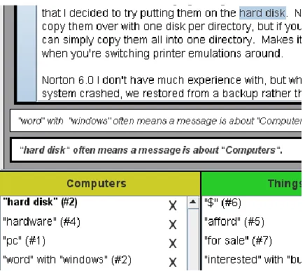
For the study, we created a software prototype allowing participants to flexibly provide feature labels within a message reader interface. The prototype window had two main areas (Figure 3): the document display and the feature display. The document display area, which was the participants’ main interface for labeling features, showed the list of documents, each with its newsgroup label, in a scrollable panel. Participants could highlight portions of the document text with the cursor (as in Figure 3) that they thought were characteristic of the document’s newsgroup. Participants could create multiple suggestions for each document, and could also delete or modify their suggestions. Participants were given great flexibility in identifying features: they were allowed to highlight

anything in the document text, including single words, punctuation, continuous phrases, and non-contiguous words or phrases.

4.2.3 Algorithm Evaluation

We used participant-provided feature labels instead of the oracle feature labels to compare the performance of LWLR-FL and LWLR-SS-FL against the other supervised and semi-supervised methods described in Section 4.1.1 and 4.1.2. Participants could label features by highlighting any text—they did not have to know whether their feature existed before (recall that we used a vocabulary of unigrams with stopwords removed for the original representation). If a participant created a new feature, we added it to the document representation used for that participant’s data and created a corresponding feature label for it. Using these data, we analyzed two variants of this experiment: one variant used participants’ labels on existing features only, and the other used all features that participants provided.

4.2.4 Feature Characteristics Analysis

In addition to information gain, we computed relatedness as a measure between the features and their associated class labels that participants provided. Informally, relatedness of a feature to a topic is how closely it represents a topic’s subject matter.

We used ConceptNet to provide us with a measure of relatedness. ConceptNet [21] is a commonsense knowledgebase, generated automatically from sentences

Fig. 3. (Top): The document display allows highlighting any text, e.g. “hard disk” in a message labeled Computers (message label cropped off for

entered by users of the Open Mind Common Sense Project. ConceptNet can support textual reasoning such as topic-jisting and analogy-making by providing relationships between words and phrases. AnalogySpace [34], which is based on ConceptNet, provides a similarity score (-1 to 1) between two features e.g. “horse” and “cow” are similar to a degree of 0.89 yet “pencil” and “cow” are not very related with a similarity score of -0.01. We used this similarity score as a measure of relatedness between features and topics.

To obtain similarity scores, we used the following process. We excluded punctuation or symbols e.g. “$”, “?”, etc, as ConceptNet does not contain information on punctuation. We then normalized the features by using the in-built ConceptNet function which takes a string and converts it into its most “natural” state, removing modifiers, inflections, and stop words. For example “asking”, when normalized, is “ask”. If the function call produced no normalized output, it was entered into ConceptNet in its unmodified form. For non-continuous words, we calculated a similarity score for each individual word, then we used the maximum score of all words in the feature. When participants provided compound words (e.g. “diet/exercise”) and phrases (e.g. “hard disk”), we calculated a similarity score for each individual word and the original given feature, again using the maximum as the final score.

5 Results and Discussion

5.1 Supervised Learning

In this section, we present results on the effectiveness of the LWLR-FL algorithm, first for simulated, ideal circumstances with features provided by a feature oracle, and, second, when feature labels were provided by participants. Also, with an eye toward eventual use in real settings, we investigated the characteristics of end-user feature labels and the algorithm’s sensitivity to parameter settings.

5.1.1 Oracle Feature Labels

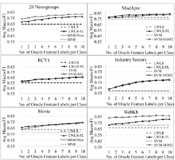
Figure 4 presents the effects of incrementally adding the top ten oracle feature labels per class over a variety of algorithms and data sets. We evaluated the algorithms in terms of the average macro-average F1 score (abbreviated to macro-F1), where the average was computed over the 30 random training/validation/testing splits. As more oracle feature labels were added, the average macro-F1 scores generally increased for all algorithms.

baseline for LWLR-FL. A “plain” linear SVM was used as a baseline algorithm for the SVM-based algorithms while a “plain” Naïve Bayes (NB) was used as a baseline for MNB/Priors.

The benefit of incorporating feature labeling can be expressed as the improvement in macro-F1 score over the feature labeling algorithm’s baseline when ten oracle feature labels were added. We denote this improvement as

baseline and show the average baseline at the bottom of Table 2. The average

baseline over the 30 runs was a statistically significant improvement for

LWLR-FL, MNB/Priors, and the best SVM-based methods in all cases (Wilcoxon signed-rank test, p < 0.05), indicating that feature labeling does indeed improve performance. The MNB algorithm had the lowest Macro-F1 score out of the baseline algorithms in four of the six datasets, but with feature labeling, the MNB/Priors algorithm produced the largest average baseline out of all the feature

labeling algorithms.

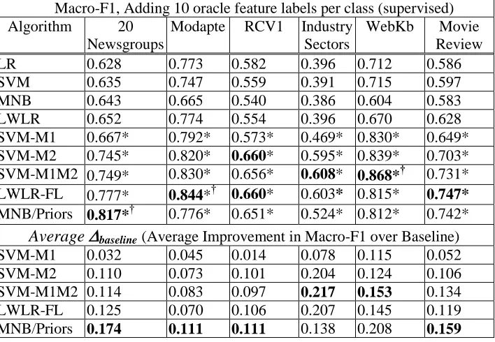
Table 2 also summarizes the macro-F1 scores for the different algorithms over the six datasets when ten oracle feature labels per class were added. Table 2 also includes the performance of global Logistic Regression (LR) for comparison. LR outperformed or came close to matching the performance of LWLR on four datasets (Modapte, RCV1, IndustrySectors, WebKb), indicating that a global fit was sometimes better than a local one, but with feature labeling, LWLR-FL ultimately outperformed LR on these four datasets. Overall, LWLR-FL was the best performing feature labeling algorithm on three (Modapte, RCV1 and Movie Review) of the six datasets, although the results were not statistically significant from the next closest feature labeling algorithm in all cases and it tied SVM-M1M2 on RCV1. MNB/Priors was the best performing algorithm on the 20 Newsgroups dataset while SVM-M1M2 was the best performing algorithm on the WebKb and Industry Sectors datasets.

Macro-F1, Adding 10 oracle feature labels per class (supervised) Algorithm 20

Newsgroups

Modapte RCV1 Industry Sectors

WebKb Movie Review

LR 0.628 0.773 0.582 0.396 0.712 0.586

SVM 0.635 0.747 0.559 0.391 0.715 0.597

MNB 0.643 0.665 0.540 0.386 0.604 0.583

LWLR 0.652 0.774 0.554 0.396 0.670 0.628

SVM-M1 0.667* 0.792* 0.573* 0.469* 0.830* 0.649* SVM-M2 0.745* 0.820* 0.660* 0.595* 0.839* 0.703* SVM-M1M2 0.749* 0.830* 0.656* 0.608* 0.868*† 0.731* LWLR-FL 0.777* 0.844*† 0.660* 0.603* 0.815* 0.747*

MNB/Priors 0.817*† 0.776* 0.651* 0.524* 0.812* 0.742*

Average



SVM-M1 0.032 0.045 0.014 0.078 0.115 0.052

SVM-M2 0.110 0.073 0.101 0.204 0.124 0.106

SVM-M1M2 0.114 0.083 0.097 0.217 0.153 0.134

LWLR-FL 0.125 0.070 0.106 0.207 0.145 0.119

MNB/Priors 0.174 0.111 0.111 0.138 0.208 0.159

Table 2. Results of supervised feature labeling algorithms incorporating 10 oracle feature labels per class. The symbol * denotes values that are significantly greater than baseline algorithms and † denotes values that are

significantly greater than all other algorithms at the 0.05 level (Wilcoxon signed-rank test, p < 0.05). The best F1 score and



5.1.2 User Study Results

The results in Section 5.1.1 indicate that with ideal feature labels, incorporating feature label information improved the classifier, especially when the LWLR-FL algorithm was used. We now turn our attention to the effects of feature labels provided by actual end users, which we expected to have less of a gain than the idealized oracle feature labels.

5.1.2.1 End-user Feature Labels

Figure 5 illustrates the performance of the feature labeling algorithms on end-user feature labels. In our analysis, SVM-M1M2 consistently outperformed M1 and M2. Therefore, to avoid clutter in the graphs, the only SVM-variant we show results for is SVM-M1M2. For reference, the leftmost group duplicates the eight oracle feature labels per class results from Section 5.1. We chose eight oracle feature labels per class as a reference because on average, participants provided this many feature labels per class. The middle group presents results when only feature labels on existing features were considered (i.e. feature labels on features created by participants were ignored). Finally, the rightmost group of results illustrates the macro-F1 scores when all feature labels were considered, including the new features created by the participant.

As we expected, gains from labels entered by the end users did not match those of the oracle feature labels. Some differences were as large as approximately 10% in average macro F1-score. These differences point out the importance of including evaluations with real end users for this type of problem.

Fig. 5. Average macro-F1 scores for the 20 Newsgroups dataset when incorporating end user feature labels through supervised feature labeling: (left) incorporating 8 oracle feature labels per class from Section 5.1, (middle) incorporating end-user feature labels only for

Evaluations in idealized conditions produced results about an algorithm’s potential, and hence were overly optimistic, as seen by comparing Figure 5’s leftmost bars with the bars to the right.

Participants were able to provide useful feature labels in our experiments, as can be seen in Figure 5. All algorithms outperformed their baselines by a statistically significant margin (Wilcoxon signed-rank test, p < 0.05) for the “all” features case, but only LWLR-FL and MNB/Priors were significantly better with “existing” features (Wilcoxon signed-rank test, p < 0.05). The best performing algorithm overall was MNB/Priors. Both MNB/Priors and LWLR-FL produced larger improvements over their baselines than SVM.M1M2, indicating that they were more robust to lower quality feature labels supplied by end users.

Feature labels were useful when labels were incorporated for existing features only (Figure 5 middle) and also when labels were incorporated for all features, including those created by end users (Figure 5 right). In fact, there was a slight increase in average macro-F1 when we included features created by end users, indicating that end users could indeed create predictive features for the 20 Newsgroups dataset. This result is encouraging for the deployment of feature labeling algorithms with ordinary end users but further investigation is needed to determine how beneficial end-user feature engineering will be on other real-world datasets.

5.1.2.2 Supervised-Learning: Sensitivity Analysis

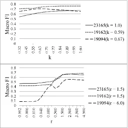
The sensitivity of LWLR-FL depends primarily on the kernel width k, which defines the neighborhood around a query point. The best k2 for a training set was found using grid search in the range 0.1 - 1.0 (values larger than 1.0 generally reduced macro-F1). Figure 6 (top) illustrates the variation in macro-F1 score for LWLR-FL for three participants when we vary k. In this analysis, we kept the regularization parameter in LWLR set to 1.0. The participants were chosen to represent extreme conditions, one having highest, one having average, and one having lowest gains in macro-F1. The macro-F1 score was computed on each participant’s holdout test set. The variation of macro-F1 scores for LWLR-FL was smooth with varying k and tended to be within a narrower range. We found empirically that a “default” value of √ yielded reasonably good macro-F1 scores.

For comparison, we include a sensitivity analysis of the SVM-M1M2 algorithm. Figure 6 (bottom) illustrates the variation of macro-F1 scores on the same three participants when we varied the r parameter for the SVM-M1M2 method, which was the most sensitive parameter. In this graph, we held the a, d,

Fig. 6. Variation of macro-F1 with k for LWLR-FL (top) and with r for

SVM-M1M2 (bottom). Data is plotted for the same three participants. The parameter value chosen after tuning on a validation set of size 24 (as described in Section 4.2) is shown for each participant in brackets in the plot

and C parameters fixed to their values tuned on the validation set. Although the scales of the parameters are difficult to compare head-to-head, Figures 6 (top) and (bottom) show that SVM-M1M2 was more sensitive to the r parameter than LWLR-FL was with the k parameter. Even within a small radius around the tuned value, the variation in macro-F1 for SVM-M1M2 covered a larger range. These results suggest that LWLR-FL is robust to changes in the k parameter and suitable for real-world deployments in which a large number of training instances may not be available.

5.1.2.3 Characteristics of End-user Feature Labels

Our results showed that features provided by end users could improve the accuracy of feature labeling algorithms. To understand what kinds of features an algorithm should expect from end users, we investigated the types of features our participants provided, the amount of gain each type contributed, and a possible basis on which participants may have chosen these features.

Using word clouds, Figure 7 illustrates the features from each newsgroup that were most commonly labeled by participants as a whole. These word clouds give an indication as to how participants collectively viewed the features that were indicative of the content of the newsgroup. Figure 7 shows that participants focused on a much smaller set of words to label for misc.forsale and sci.space

than for comp.sys.ibm.pc.hardware and sci.med. The more diffuse word clouds consisted of technical jargon, as participants felt these specific terms were more predictive as to the content of the newsgroup. Despite the variety in the nature of these newsgroups, participants in our study were able to provide informative feature labels and ultimately improve the classifiers.

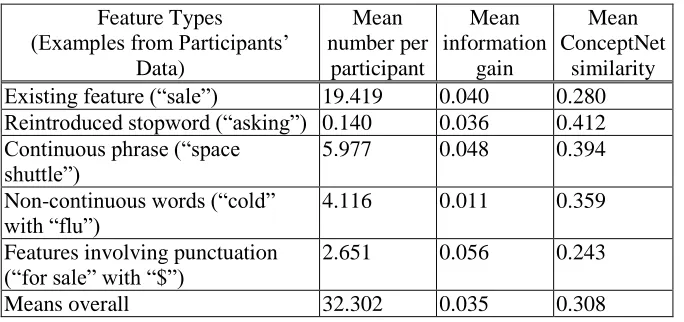
Table 3 shows the frequencies of the types of features participants chose. The most common type, accounting for about 60% of the features, was features that the algorithm already knew existed, in the form of unigrams (row 1 in the table). Some of these had information gains comparable to features chosen by the oracle (for example, 10 of the 43 participants chose the top oracle feature “sale”), although overall, participants’ features had a somewhat lower average information gain (0.035) than the oracle’s (0.078).

These computations showed that participants chose features with higher relatedness (average 0.308) than those chosen by the oracle (average 0.231). In general, the participants’ choices of features with high relatedness helped as relatedness has a relationship with information gain (linear regression, R2=0.04, p<0.001). This suggests possible directions for designers of interactive intelligent systems to use in encouraging end users to usefully label features. For example, relatedness could be used to suggest relevant predictive features for end users to label, thereby helping them overcome their known difficulty of knowing where to look when trying to provide guidance to the system (e.g., “What kind of words should we tell the computer [relating] to Systems?” [14].)

Finally, note that 40% of participants’ feature choices were not known to the algorithm previously, as rows 2-5 in Table 3 show. Some of these features, such as stopwords and punctuation, had previously been removed from the vocabulary but were partially reintroduced by participants. Features such as multiple word phrases (n-grams) and non-continuous words (feature combinations) cannot be addressed by simply adding all possibilities (e.g., all n-grams) as features to the learning algorithm, because doing so would explode the feature representation, making learning infeasible. In addition, for applications that customize themselves to the end user, these specific features may be unique to those end users and thus not foreseeable by the algorithm designer prior to deployment. Thus, allowing end users to provide features not originally in the learning algorithm’s data representation is an important benefit, which we have only begun to investigate in end-user feature labeling.

Fig. 7. Top Features Selected by Participants for

comp.sys.ibm.pc.hardware (Top Left), misc.forsale (Top Right), sci.med

5.2 Semi-supervised Learning

Having presented results for the supervised feature labeling setting, we now present results for the semi-supervised setting when an unlabeled pool of data was available during training. As before, we will first show results for the oracle study and then show results for feature labels harvested from real users during the user study.

5.2.1 Oracle Feature Labels

Figure 8 and Table 4 depict the results of adding 10 oracle feature labels per class to the semi-supervised feature labeling algorithms. LWLR-SS-FL outperformed the other algorithms on the 20 Newsgroups, Modapte, and Industry Sectors datasets, with statistically significant improvements over GE and SVM-M3 (Wilcoxon signed-rank test, p < 0.05). GE, however, had the best macro-F1 on the WebKb and Movie Review datasets with statistically significant improvements over the second best algorithm (Wilcoxon signed-rank test, p< 0.05). For the RCV1 dataset, SVM-M3 had the best macro-F1.

Past work in semi-supervised learning (eg. [3]) has indicated that the label diffusion approach to semi-supervised learning was successful if the data had a smooth underlying manifold structure in which instances from the same class were close enough to each other to allow labels from labeled training instances to propagate to unlabeled instances that were of the same class. Label diffusion performed poorly if the “islands” of data instances from one class fell in between “islands” of data instances from another class on the manifold structure. We believe that the poor behavior of LWLR-SS-FL on WebKb and Movie Review

Feature Types (Examples from Participants’

Data)

Mean number per

participant

Mean information

gain

Mean ConceptNet

similarity Existing feature (“sale”) 19.419 0.040 0.280 Reintroduced stopword (“asking”) 0.140 0.036 0.412 Continuous phrase (“space

shuttle”) 5.977 0.048 0.394

Non-continuous words (“cold” with “flu”)

4.116 0.011 0.359

Features involving punctuation (“for sale” with “$”)

2.651 0.056 0.243

Means overall 32.302 0.035 0.308

Table 3. Labeled features per participant by type. All types are disjoint. Only 6 of the 43 users introduced removed stopwords, and each

datasets was due to these datasets having an underlying structure that did not satisfy this particular assumption of label diffusion.

Having investigated both supervised and semi-supervised learning for Oracle feature labeling, we can now compare the relative benefits of augmenting learning from labeled training instances using feature labeling, unlabeled data, and a combination of the two. Table 5 and Figure 9 show the change in macro-F1 over the baseline LWLR algorithm when feature labeling, semi-supervised learning, and both feature labeling and semi-supervised learning were added. In general, information from feature labels helped learning more than information from unlabeled data. In fact, in four datasets (Modapte, RCV1, WebKb, and

Macro F1, Adding 10 Oracle Feature Labels per class (Semi-supervised) Algorithm 20

Newsgroups

Modapte RCV1 Industry Sectors

WebKb Movie Review

SVM 0.635 0.747 0.559 0.391 0.715 0.597

MNB 0.643 0.665 0.540 0.386 0.604 0.583

LWLR 0.652 0.774 0.554 0.396 0.670 0.628

LWLR-SS-FL 0.900† 0.844† 0.643 0.703† 0.745 0.708

SVM-M3 0.809 0.827 0.649 0.659 0.851 0.758

GE 0.823 0.766 0.556 0.663 0.876† 0.782†

MNB/Prior+EM 0.806 0.431 0.535 0.460 0.601 0.744

Table 4. Results of incorporating 10 oracle features per class through semi-supervised feature labeling for all six datasets. The symbol †denotes values

that are significantly greater than all other algorithms at the 0.05 level (Wilcoxon signed-rank test, p < 0.05). Results for the baseline SVM and

LWLR algorithms are included for reference.

Fig. 8. Average macro-F1 scores for incorporating 10 Oracle feature labels through semi-supervised feature labeling for the six datasets used in our

Movie), the unlabeled data caused the performance of LWLR-SS to degrade below that of the baseline supervised learning LWLR algorithm. Surprisingly, combining feature labeling with semi-supervised learning overcame this deficit, resulting in better performance than the baseline. Semi-supervised feature labeling, however, did not necessarily outperform supervised feature labeling. On three datasets (RCV1, WebKb, Movie Review), LWLR-SS-FL performed worse than LWLR-FL. Overall, however, incorporating information from feature labels always improved performance in both the supervised and semi-supervised settings, as one can see by the improvement of LWLR-FL over LWLR and the improvement of LWLR-SS-FL over LWLR-SS.

We repeated this experiment using feature labeling algorithms based on the MNB algorithm as illustrated in Figure 10. Supervised feature labeling was the best performing algorithm, consistently producing large improvements over the

Macro F1, Adding 10 Oracle Features per class (Semi-supervised) Algorithm 20

Newsgroups

Modapte RCV1 Industry Sectors

WebKb Movie Review

LR 0.623 0.773 0.582 0.396 0.712 0.586

LWLR 0.652 0.774 0.554 0.396 0.670 0.628

LWLR-FL 0.777* 0.844* 0.660* 0.603* 0.815* 0.747*

LWLR-SS 0.789* 0.723 0.512 0.430* 0.452 0.468

LWLR-SS-FL 0.900* 0.840* 0.644* 0.703* 0.745* 0.691*

Table 5. Results of adding 10 oracle features per class for all six datasets for algorithms that are variants of logistic regression. The symbol * denotes values that are significantly greater than the baseline LWLR algorithm at

the 0.05 level

(Wilcoxon signed-rank test, p < 0.05)

baseline MNB algorithm in all cases. Semi-supervised learning (without feature labeling), on the other hand, resulted in worse performance than the baseline algorithm for four datasets (Modapte, RCV1, Industry Sectors and WebKb). Unlike LWLR, semi-supervised learning with feature labeling only outperformed the baseline algorithm in three datasets (20 Newsgroups, Industry Sectors and Movie Review) and performance degraded below the baseline in the other three datasets, including a large drop in macro-F1 of 0.23 for Modapte.

Overall, the results for feature labeling using the LWLR and MNB variants clearly demonstrate that feature labeling is the more reliable alternative to augment the learning process than using unlabeled data in a semi-supervised setting, which can degrade learning. Using a combination of semi-supervised learning and feature labeling can overcome the degradation in performance from the unlabeled examples if LWLR-SS-FL is used, but the results are mixed using MNB/Prior+EM.

Macro F1, Adding 10 Oracle Features per class (Semi-supervised)

Algorithm 20

Newsgroups

Modapte RCV1 Industry Sectors

WebKb Movie Review

MNB 0.643 0.665 0.54 0.386 0.604 0.583

MNB/Priors 0.817* 0.776* 0.651* 0.524* 0.812* 0.742* MNB+EM 0.663 0.403 0.427 0.333 0.518 0.607 MNB/Prior+EM 0.806* 0.431 0.535 0.46 0.601 0.744*

Table 6. Results of adding 10 oracle features per class for all six datasets. The symbol * denotes values that are significantly greater than the baseline

MNB algorithm at the 0.05 level (Wilcoxon signed-rank test, p < 0.05)

5.2.2 End-User Feature Labels

As before, we would like to evaluate the semi-supervised feature labeling algorithms using feature labels provided by actual end users rather than using idealized feature labels generated by an oracle. Using feature labels harvested from end users in the study from Section 4.2, we evaluated LWLR-SS-FL against SVM-M3, GE and MNB/Priors+EM.

Figure 11 summarizes the results from this experiment. We also plot the results using the LWLR and SVM baselines (from Section 5.1.1) as a reference. Results with 8 oracle feature labels per class are shown in the leftmost group. As before, we divide the results into the “existing” features group, in which feature labels were only permitted on existing features, and the “all” features group, in which new features that participants created were added to the data representation and then labeled. Results for “existing” and “all” features are

shown in the middle and rightmost groups respectively.

For SVM-M3, end-user feature labels degraded the performance of the algorithm below the SVM baseline in this semi-supervised setting, while LWLR was more robust. GE performed the worst out of all the other algorithms with end- user feature labels, indicating that it was very sensitive to the quality of feature labels. The poor performance of GE was due to the lower quality end-user feature labels being the only source of supervision for GE’s learning process. Furthermore, in past work, GE performed very well when users were guided to provide feedback on features selected by topic models or by active-learning [10], unlike in our setup where the users had no guidance at all as to which features to label. Both LWLR-SS-FL and MNB/Priors+EM improved upon their respective

Fig. 11. Results of Semi-supervised Algorithms with User Feature Labels: (Left) incorporating 8 oracle feature labels per class from Section 5.2.1, (Middle) incorporating end-user feature labels only for existing features,

baseline algorithms with end user feature labels. LWLR-SS-FL significantly outperformed other algorithms on the “all” feature cases (Wilcoxon signed-rank test, p < 0.05).

When compared against the gains from supervised feature labeling (Figure 5), SVM-M3 was more sensitive to lower quality feature labels from participants than its supervised learning counterpart (SVM-M1M2); SVM-M1M2 performed better than SVM-M3 and resulted in an improvement over the SVM baseline. Similarly, MNB/Priors+EM performed slightly worse than its supervised learning counterpart (MNB/Priors). Unlike the former two algorithms, LWLR-SS-FL outperformed its supervised learning counterpart (LWLR-FL) in all cases.

5.2.3 Sensitivity Analysis

LWLR-SS-FL introduces two new parameters – the label diffusion kernel width (k), and the number of nearest neighbors (#nn). In our experiments, we set

k to √ and #nn to 100 for all datasets in LWLR-SS and LWLR-SS-FL. Here, we present the sensitivity plots for k and #nn on three datasets – 20 Newsgroups, ModApte, and WebKB. In the sensitivity analysis of parameter k, we kept #nn

Fig. 12. Sensitivity of LWLR-SS-FL to number of nearest neighbors #nn

constant at 100 and varied k in the range [0-1]. In the sensitivity analysis of parameter #nn, we kept k constant at √ and varied #nn in the range [5-100].

Figure 12 (top) shows that the algorithm was not very sensitive to the number of nearest neighbors (#nn). However, the algorithm was more sensitive to k as can be seen in Figure 12 (bottom). Since we used TFIDF-L2 normalization, a kernel of width 1.0 spanned across all instances resulting in a “global” fit. We can see that these datasets had similar localized regions where label diffusion helped. The performance of the algorithm on 20 Newsgroups hardly improved beyond k=0.5 which might suggest that instances in this dataset formed very few compact clusters in the feature space and the seed (labeled training) instances managed to cover most of them. In WebKB on the other hand, performance degraded till k=0.4 and then recovered as k increased to 1 and beyond. This suggests that the WebKB categories might have formed a large number of small clusters that were intermingled and the seed instances had not been able to cover all small clusters. ModApte showed similar characteristics as WebKB, but managed to avoid the steep degradation in performance as observed in WebKB at around k=0.4. This could have been because ModApte had fewer instances than WebKb and hence was sparser in the feature space.

5.2.4 Discussion and Future Work

With oracle feature labels, the semi-supervised feature labeling algorithms produced a dramatic increase over their respective baselines, which was similar to results reported in previous work [29, 10]. However, with the lower quality features that came from real users, some semi-supervised feature labeling algorithms performed worse than algorithms that ignore the feature labels eg. SVM-M3 performed worse than its SVM baseline. Past work in semi-supervised learning [42, 40] has shown that semi-supervised learning does not always produce an improvement in performance over supervised learning. In his survey on semi-supervised learning [40], Zhu pointed out that a mismatch between model assumptions and the problem structure could produce worse performance than supervised learning, but “detecting this mismatch in advance is hard and remains an open problem”.