Tests for skewness and kurtosis in the one-way error component model

City, University of London Institutional Repository

Citation

: Galvao Jr, A. F., Montes-Rojas, G., Sosa-Escudero, W. and Wang, L. (2013).

This is the accepted version of the paper.

This version of the publication may differ from the final published

version.

Permanent repository link:

Link to published version

: http://dx.doi.org/10.1016/j.jmva.2013.07.002

Copyright and reuse:

City Research Online aims to make research

outputs of City, University of London available to a wider audience.

Copyright and Moral Rights remain with the author(s) and/or copyright

holders. URLs from City Research Online may be freely distributed and

linked to.

Tests for skewness and kurtosis in the one-way error

components model

Antonio F. Galvao

Gabriel Montes-Rojas

Walter Sosa-Escudero

Liang Wang

July 2, 2013

Abstract

This paper derives tests for skewness and kurtosis for the panel data one-way error components model. The test statistics are based on the between and within transforma-tions of the pooled OLS residuals, and are derived in a moment conditransforma-tions framework. We establish the limiting distribution of the test statistics for panels with large cross-section and fixed time-series dimension. The tests are implemented in practice using the bootstrap. The proposed methods are able to detect departures away from nor-mality in the form of skewness and kurtosis, and to identify whether these occur at the individual, remainder, or both error components. The finite sample properties of the tests are studied through extensive Monte Carlo simulations, and the results show evidence of good finite sample performance.

Key Words: Panel data, Error components, Skewness, Kurtosis, Normality

AMS subject classifications: 62F03, 62F05, 62H15

∗_{Corresponding author: Department of Economics, University of Iowa, W210 Pappajohn Business} Build-ing, 21 E. Market Street, Iowa City, IA 52242. E-mail: antonio-galvao@uiowa.edu

†_{Department of Economics, City University London, Northampton Square, London EC1V 0HB, UK.} E-mail: Gabriel.Montes-Rojas.1@city.ac.uk

‡_{Department of Economics, Universidad de San Andr´es, Argentina and CONICET. E-mail:}

wsosa@udesa.edu.ar

1

Introduction

The need to check for non-normal errors in regression models obeys to both methodological and conceptual reasons. From a strictly methodological point of view, lack of Gaussianity sometimes harms the reliability of simple estimation and testing procedures, and calls for either better methods under alternative distributional assumptions, or for robust alternatives whose advantages do not depend on distributional features. Alternatively, whether errors should be more appropriately captured by skewed and/or leptokurtic distributions may be a statistical relevant question per se.

The normality assumption also plays a crucial role in the validity of specification tests. Blanchard and M´aty´as (1996) examine the consequences of non-normal error components for the performance of several tests. In a recent application, Montes-Rojas and Sosa-Escudero (2011) show that non-normalities severely affect the performance of the panel heteroskedas-ticity tests by Holly and Gardiol (2000) and Baltagi, Bresson and Pirotte (2006), in line with the results of Evans (1992) for the cross-sectional case. Despite these concerns the Gaussian framework is widely used for specification tests in the one-way error components model; see, for instance, the tests for spatial models in panel data by Baltagi, Song and Koh (2003), and Baltagi, Song, Jung, and Koh (2007).

Even though there is a large literature on testing for skewness and kurtosis in cross-sectional and time-series data, including Ergun and Jun (2010), Bai and Ng (2005), Pre-maratne and Bera (2005), Dufour, Khalaf and Beaulieu (2003), Bera and PrePre-maratne (2001), Henze (1994) and Lutkepohl and Theilen (1991) to cite a few of an extensive list that dates back to the seminal article by Jarque and Bera (1981), results for panel data models are scarce. A natural complication is that, unlike their cross-section or time-series counterparts, in simple error-components models lack of Gaussianity may arise in more than one compo-nent. Thus, an additional problem to that of detecting departures away from normality is the identification of which component is causing it. Previous work on the subject include Gilbert (2002), who exploits cross-moments, and Meintanis (2011), who proposes an omnibus-type test for normality in both components jointly based on empirical characteristic functions.

remainder components, separately and jointly. We show that under the corresponding null hypothesis the limiting distributions of the tests are asymptotically normal. To obtain the asymptotic distributions of the test statistics, we consider the most important case where the number of individuals, N, goes to infinity, but the number of time periods, T, is fixed and might be small. The proposed methods and associated limiting theory are important in practice because, in the panel data case, the standard Bera-Jarque test is not able to disentangle the departures of the individual and remainder components from non-Gaussianity.

The proposed tests are implemented in practice using a bootstrap procedure. Since the tests are asymptotically normal, the bootstrap can be used to compute the corresponding variance-covariance matrices of the statistics of interest and carry out inference. In partic-ular, the tests are implemented using a cross-sectional bootstrap. We formally prove the consistency of the bootstrap method applied to our case of short panels.

A Monte Carlo study is conducted to assess the finite sample performance of the tests in terms of size and power. The Monte Carlo simulations show that the proposed tests and their bootstrap implementation work well for both skewness and kurtosis, even in small samples similar to those used in practice. The results confirm that the test for the individual specific component depends on the cross-section dimension only, and hence it is invariant to the time-series dimension. The proposed tests detect departures away from the null hypothesis of skewness and/or kurtosis in each component, and are robust to the presence of skewness and/or kurtosis in the other component.

Finally, to highlight the usefulness of the proposed tests, we apply the new tests to the Fazzari, Hubbard and Petersen (1988) investment equation model, in which firm investment is regressed on a proxy for investment demand (Tobin’s q) and cash flow.

2

Skewness and kurtosis in the one-way error

compo-nents model

2.1

The model and the hypotheses

Consider the following standard panel data one-way error components model

yit =α0+x>itβ0+uit, uit=µi +νit, i= 1, ...N, t= 1, ..., T, (1)

where α0 is a constant, β0 is a p-vector of parameters, and µi, νit, and xit are copies of

random variables µ, ν, and x, respectively. As usual, the subscript i refers to individual and t to time. Here µi and νit refer to the individual-specific and to the remainder error

component, respectively, both of which have mean zero.

The quantities of interest are each component skewness,

sµ=

µ3

σ3

µ

= E[µ

3_]

(E[µ2_])3/2, and sν =

ν3

σ3

ν

= E[ν

3_]

(E[ν2_])3/2,

and kurtosis,

kµ=

µ4

σ4

µ

= E[µ

4_]

(E[µ2_])2, and kν =

ν4

σ4

ν

= E[ν

4_]

(E[ν2_])2.

We are interested in testing for skewness and kurtosis in the individual-specific and the remainder components, separately and jointly. When the underlying distribution is normal, the null hypotheses of interest become Hsµ

0 : sµ = 0 and H0sν : sν = 0 for skewness and

Hkµ

0 : kµ = 3 and H0kν : kν = 3 for kurtosis. We also consider testing for skewness and

kurtosis jointly. Under normality, the null hypotheses for these cases are given by

Hsµ&kµ

0 :sµ= 0 andkµ= 3,

Hsν&kν

0 :sν = 0 andkν = 3.

It is common in the statistics and econometrics literature to check for the third and fourth moment of a random variable and compare them with the corresponding values of a normal distribution. This corresponds to a test for normality of each component. Thus, the last hypotheses can be regarded as tests for normality. The following sections develop the corresponding test statistics.

We introduce the following notation. ui ≡ T−1

PT

t=1uit are the between residuals, and

e

Similarly, xi ≡ _T1

PT

t=1xit. In general, a line over a variable with a subscript i indicates a

group average. A tilde will denote variables expressed as deviations from the corresponding group mean. A line over a variable without a subscript indicates the total average across

i and t, e.g., x ≡ 1

N T

PN

i=1

PT

t=1xit. Also, for a generic random vector Xi indexed by i,

let _E[Xi] denote _N1 PN_i=1Xi. Let buit =yit−αb0−x

>

itβb be the pooled ordinary least squares

(OLS) residuals, where βb is the pooled OLS estimator. It is straightforward to show that

the slope coefficients admit an asymptotic representation such that√N(βb−β₀) = O_p(1).

2.2

Skewness

In this section we develop statistics for testing skewness. In order to derive moment con-ditions to test for skewness in each component, consider the cube of the between residuals,

u3_i = (µi +νi)3 = µ3i +ν3i + 3µ2iνi + 3µiν2i. Taking expectations on both sides of the last

equation, we have

E[u3_i] =µ3+T−2ν3.

The cube of thewithin residuals is given by u_e3_it = (νit−νi)3 =νit3 −ν3i −3νit2νi+ 3νitν2i, and

after taking expectations

E[_eu3_it] =ν3 −T−2ν3−3T−1ν3+ 3T−2ν3 =ν3 1−3T−1+ 2T−2

.

Solving these equations forν3 and µ3, we obtain

ν3 =

1

1−3T−1_{+ 2T}−2E[ue

3

it],

µ3 = E[u3i]−

1

T2_{−3T + 2}E[ue

3

it].

Therefore, the tests for skewness in each component make use ofu3_i and_eu3

it. To carry tests in

practice, we need to construct the sample counterpart of these equations. First, we rewrite the equations. Recall that u_e3_it = (uit −ui)3 = u3it −u3i −3u2itui + 3uitu2i, and that in the

one-way error components model (using the assumptions below), for each i, the {_euit}’s are

identically distributed, then it follows that E[_eu3

it] = E[eu

3

i] whereue

3

i = T1

PT

t=1ue

3

it, and

ν3 =

1

1−3T−1_{+ 2T}−2E[u 3

i −3uiu2i + 2u

3

i],

µ3 =

T2 −3T T2_{−3T + 2}E[u

3

i]−

1

T2_{−3T + 2}E[u 3

However, the above equations are functions of the unobservable innovations. Thus, we define _bν3 and µb3 as the estimators of ν3 and µ3, respectively, which are constructed using b

uit, the OLS residuals. Then, we have that

b

ν3 =

1

1−3T−1_{+ 2T}−2E[bu

3

i −3buibu

2

i + 2ub

3

i],

b

µ3 =

T2−3T T2_{−3T + 2}E[ub

3

i]−

1

T2_{−3T + 2}E[ub

3

i −3ubiub

2

i].

Finally, the following statistics are useful to construct tests for skewness

d

SKν =b

ν3

b

σ3

ν

, (2)

d

SKµ=b

µ3

b

σ3

µ

. (3)

In Section 3 we construct tests for skewness based on these statistics, and derive their limiting distributions under some regularity conditions (Assumptions 1 and 2, in the next section). The estimatorsσ_b3

ν andσb

3

µ are given in Appendix A1. It is easy to show that under

Hsν 0 , SKdν

p

→0. Note that the use of the within transformation to construct the estimator implies that SKd_ν is not affected by skewness (or kurtosis) in µ.

Consider now the estimator for skewness in the individual component, sµ. As in the

previous case,SKd_µ

p

→sµ, as N → ∞and fixed T. In addition, under the null hypothesis of

normalityHsµ 0 ,SKdµ

p

→0. Note thatSKdµis robust to the presence of skewness (or kurtosis)

in the remainder component, sν, even in small panels, i.e., finite T.

2.3

Kurtosis

In order to derive similar statistics to test for kurtosis, consider the fourth power of the

between residuals, u4

i = (µi+νi)4 =µ4i +ν4i + 4µ3iνi+ 4µiνi3+ 6µ2iν2i. Taking expectations

of u4_i we obtain

E[u4_i] =µ4+T−3(ν4+ 3(T −1)σ4ν) + 6T

−1

σ2_µσ_ν2.

Consider now the fourth power of thewithin residuals, u_e4_it = (uit−ui)4 =νit4 +ν4i −4νit3νi−

4νitν3i + 6νit2ν2i. Taking expectations ofue

4

it we obtain

E[u_e4_it] =ν4 1−4T−1+ 6T−2−3T−3

+σ_ν4(T −1)(6T−2−12T−3).

These expectations are linear functions of ν4 and µ4, suggesting, again, that tests for

kurtosis of each component can be based onu4

i and ue

4

forν4 and µ4 and noting that eu

4

it= (uit−ui)4 =u4it+u4i −4u3itui−4uitu3i + 6u2itu2i, it follows

that

ν4 =

E[_eu4_it]

1−4T−1_{+ 6T}−2_−3T−3 −

(T −1)(6T−2−12T−3) 1−4T−1_{+ 6T}−2_−3T−3σ

4

ν

= E[u

4

i]−4E[u3iui] + 6E[u2iu2i]−3E[u4i]

1−4T−1_{+ 6T}−2 _−3T−3 −

(T −1)(6T−2−12T−3) 1−4T−1_{+ 6T}−2_−3T−3σ

4

ν

µ4 = E[u4i]−T

−3

(ν4+ 3(T −1)σν4)−6T

−1

σ_µ2σ2_ν

= E[u4_i] T

3_−4T2_{+ 6T}

T3_−4T2_{+ 6T −3}−

E[u4

i]−4E[u3iui] + 6E[u2iu2i]

T3 _−4T2_{+ 6T −3}

− (T −1)(3T

3_−12T2_{+ 12T + 3)}

(T3_−4T2_{+ 6T −3)T}3 σ 4 ν− 6 Tσ 2 µσ 2 ν.

As in the previous section, the above equations are functions of the unobserved innova-tions. Define ν_b4 and µb4 as the estimators of ν4 and µ4, respectively, constructed using ubit,

the OLS residuals. Thus, we have that

b

ν4 = E

[u_b4

i]−4E[bu

3

ibui] + 6E[ub

2

iub

2

i]−3E[bu

4

i]

1−4T−1_{+ 6T}−2 _−3T−3 −

(T −1)(6T−2−12T−3) 1−4T−1_{+ 6T}−2_−3T−3bσ

4

ν

b

µ4 =E[bu

4

i]

T3_−4T2_{+ 6T}

T3_−4T2_{+ 6T −3}−

E[bu

4

i]−4E[ub

3

iubi] + 6E[bu

2

ibu

2

i]

T3 _−4T2_{+ 6T −3}

− (T −1)(3T

3_−12T2_{+ 12T + 3)}

(T3_−4T2_{+ 6T −3)T}3 bσ

4

ν−

6

Tbσ

2

µbσ

2

ν.

Finally, the following statistics are useful to construct tests for kurtosis.

d

KUν =b

ν4 b σ4 ν , (4) d

KUµ=b

µ4

b

σ4

µ

. (5)

It is important to notice that when testing for kurtosis (or both skewness and kurtosis) based on moment conditions, skewness might influence kurtosis. This might be an impor-tant drawback of these tests. Jones, Rosco, and Pewsey (2011) show that certain kurtosis measures, when applied to certain wide families of skew-symmetric distributions, display the attractive property of skewness-invariance. The authors provide quantile-based measures of kurtosis and their interaction with skewness-inducing transformations, identifying classes of transformations that leave kurtosis measures invariant.

d

KUν p

→ kν, for N → ∞ and fixed T. Then for the purpose of testing normality, under

Hkν 0 , KUd_ν

p

→ 3. Note that the statistic KUd_ν is not affected by kurtosis (or skewness) inµ.

Consistent estimators forσ_ν4 and σ_µ4 are presented in Appendix A1.

Finally, consider the estimator for kurtosis in the individual component, kµ. As before,

d

KUµ p

→ kµ, as N → ∞ and fixed T. Thus, under the null hypothesis of normality H kµ 0 ,

d

KUµ p

→ 3. As in the previous case, the statistic KUd_µ is not affected by the presence of

kurtosis (or skewness) in the remainder component.

3

Asymptotic theory

In order to implement the tests in practice we first derive the asymptotic distributions of the corresponding statistics developed in the previous section. Consider the regression model described by equation (1). We will impose the following regularity conditions to derive the asymptotic properties of the statistics.

Assumption 1. Let {µi} be a sequence of i.i.d. random variables, and {(x>it, νit)} be an

array of i.i.d. random vectors across i and t. In addition, xit, µi and νit are independent.

Both µi and νit have mean zero and finite E[µ8] and E[ν8].

Assumption 2. E[xitx>it]is a finite positive definite matrix. In addition, E[||xit||4] is finite.

Assumptions 1 and 2 are standard in the literature. The first one imposes restrictions on the sampling scheme and on the moments of the individual-specific and the remainder error components. The need to bound high order moments relates to the fact that the limiting distribution of the proposed statistics involves the variance of skewness and kurtosis statistics, which eventually depend on the sixth and eighth moments, respectively. The positive definiteness of E[xitx>it] in second assumption is a standard identification condition.

The existence of E[||xit||4] is usually required for the study of variance-covariance matrix.

Assumptions 1 and 2 guarantee that a multivariate version of the Lindeberg-L´evy central limit theorem forN → ∞ and fixedT can be used to establish the asymptotic normality of the statistics proposed in the previous section.

(2005). It is well known in this literature, and implied by the restrictions of Assumption 1, that a drawback of tests requiring high order moments is that they are not theoretically valid for numerous distributions. We will assess the finite sample performance of the proposed tests using a series of Monte Carlo experiments, reported in Section 5.

A novel aspect of our proposed framework is the ability to identify skewness and kurtosis in the error components of a standard linear panel model, separately and jointly. We provide a general framework to develop these tests and to suggest directions in which particular deviations from the model, other than non-Gaussianity, can be considered. We will focus only on the one-way error components model and leave extensions for future research. In particular, the previous assumptions could be relaxed at the cost of modeling additional terms in the expectations and variance-covariances given below for skewness and kurtosis. Suggestions for extensions are discussed in the last section.

The next theorem derives an asymptotic representation for the sample skewness and kurtosis.

Theorem 1 Under Assumptions 1 and 2, and for N → ∞ and fixed T,

(i) √N(SKd_ν −s_ν) =

B1

σ3

ν − 3sνA1

2σ2

ν 1 √ N PN

i=1Ai+op(1)

(ii) √N(SKd_µ−s_µ) =

B2

σ3

µ − 3sµA2

2σ2

µ 1 √ N PN

i=1Ai+op(1)

(iii) √N(KU[ν −kν) =

C1

σ4

ν − 2kνA1

σ2 ν 1 √ N PN

i=1Ai+op(1)

(iv) √N(KU[µ−kµ) =

C2

σ4

µ − 2kµA2

σ2 µ 1 √ N PN

i=1Ai+op(1),

where _Ai = (ui, u2i −E[u2i], u

2

i −E[u2i], u3i −E[u3i], u

3

i −E[u3i], u4i −E[u4i], u

4

i −E[u4i], u2iui −

E[u2

iui], u3iui − E[u3iui], u2iu2i − E[u2iu2i])

>_{, A}

1 = 0,₁₋1_T−1,−

1

1−T−1,0,0,0,0,0,0,0

, A2 =

0,− 1

T−1,

T

T−1,0,0,0,0,0,0,0

, B1 = (0,0,0,1,2,0,0,−3,0,0)/(1 − 3T−1 + 2T−2), B2 =

−3E[u2

i],0,0,

−1

T2_−3T+2,

T2_−3T

T2_−3T+2,0,0,

3

T2_−3T+2,0,0

, C1 = (0,(24T−2 −12T−1)σν2,(12T

−1₋

24T−2)σ_ν2,0,0,1,−3,0,−4,6)/(1−4T−1+6T−2−3T−3), andC2 =

−4E[u3_i],−(3_(TT33₋₄−12_T2T₊₆2+12_T−3)T+3)_T2−

6σ2

µ

T−1+ 6σ2

ν

T(T−1),

(3T3_−12T2_+12T+3)

(T3_−4T2_+6T−3)T2+

6σ2

µ

T−1− 6σ2

ν

T−1,0,0,

−1

T3_−4T2_+6T−3,

T3_−4T2_+6T

T3_−4T2_+6T−3,0,

4

T3_−4T2_+6T−3,

−6

T3_−4T2_+6T−3

.

Proof. See Appendix A2.

Theorem 2 Under Assumptions 1 and 2, and for N → ∞ and fixed T,

(i) √N(SKdν−sν)/

p

Ωs ν

d

→N(0,1), where Ω_νs =N V ar(SKdν);

(ii) √N(SKd_µ−s_µ)/ p

Ωs µ

d

→N(0,1), where Ωs

µ=N V ar(SKd_µ);

(iii) √N(KUdν −kν)/

p

Ωk ν

d

→N(0,1), where Ωk

ν =N V ar(KUdν);

(iv) √N(KUd_µ−k_µ)/ q

Ωk µ

d

→N(0,1), where Ω_µk =N V ar(KUd_µ).

Proof. See Appendix A3.

Theorem 2 shows that the distributions of the statistics SKd_ν, SKd_µ, KUd_ν and KUd_µ,

after centralization and standardization, are asymptotically standard normal. This result indicates that tests for skewness and/or kurtosis are simple to implement. For example, to test Hsµ

0 :sµ = 0 againstH sµ

1 :sµ 6= 0, a simple t-test can be used by standardizing the test

statistic SKd_ν by the square root of a consistent estimate of its variance, and imposing the

null hypothesis

Tsµ =SKdν/

q

V ar(SKdν) d

→N(0,1).

The critical values for this two-sided test are standard. For the case of testingHkν

0 :kν/σ4ν = 3

the procedure is analogous

Tkµ = (KUdν −3)/

q

V ar(KUd_ν)

d

→N(0,1).

The next section discusses how to implement the tests in practice.

4

Implementation

In this section, we develop a bootstrap procedure to estimate the variances of the skewness and kurtosis test statistics in practice. The implementation of the tests based on the results of Theorem 2 require a consistent estimator of the asymptotic variances of the correspond-ing statistics. Even though these variance-covariance matrices exist and are finite by the boundedness conditions in Assumption 1, they depend on the high order moments of ν and

µ. Therefore their derivation requires a cumbersome calculation. Instead, we consider the bootstrap as an alternative to estimate the corresponding asymptotic variance-covariance matrices.

(2005) discuss resampling methods for panel data when N is large but T is assumed small. Kapetanios (2008) studies the bootstrap for a linear panel data model where resampling occurs in both the cross-section and time dimensions. Goncalves (2011), allowing for both temporal and cross-sectional dependence, studies the moving block bootstrap for a linear panel data model where resampling occurs only in the time dimension.

The bootstrap method we consider is implemented by randomly drawing individuals with replacement while maintaining the time series structure unaltered. This corresponds to cross-sectional resampling in Kapetanios (2008). This method resamples {yit,xit} with

replacement from the cross-section dimension with probability 1/N, maintaining the tem-poral structure intact for each individual i. More specifically, lety∗ = (yi1, ..., yis, ..., yiN) be

the vector of bootstrap samples where each element of the vector of indices (i1, ..., iN) is

ob-tained by drawing with replacement from (1, ..., N), and each element is yis = (yis1, ..., yisT)

fors ∈(i1, ..., iN). The same vector of indices is used to obtainx∗. Therefore, each bootstrap

sample is given by{(y∗_it,x∗_it), i= 1, . . . , N;t= 1, . . . , T}.

Next we describe the bootstrap algorithm for estimating the variances in practice. We will focus on the implementation of the bootstrap procedure for testing the null hypothesis

Hsν

0 : sν = 0 with the statistic described in equation (2) and using part (i) in Theorem 2.

The algorithms for the remaining cases are analogous. To implement the test we need to compute Ωbs_ν∗, the bootstrap variance estimator. The algorithm is as follows:

1. DrawB independent bootstrap samples, (y∗_it,x∗_it)1,(y_it∗,x∗_it)2, ...,(y∗_it,x∗_it)B each consisting of i= 1, . . . , N; t = 1, . . . , T, data values as described in the previous paragraph.

2. Having obtained the resampled data, evaluate the bootstrap replication corresponding to each bootstrap sample to estimate equation (1) and compute the residuals.

3. Given the residuals for each bootstrap sample, calculate the statistic of interest as in equation (2), which is denoted bySKd

∗b

ν , b= 1, ..., B.

4. Finally, obtain Ωbs_ν∗ with the sample variance ofSKd

∗b

ν , b= 1, ..., B.

After computing this estimate, the result in part (i) of Theorem 2 can be used to construct a Wald-type test as Tsµ =NSKd

2

ν/Ωbs_ν∗. The intuition for the validity of this test is that the

limit ofV ar(SKd

∗b

ν ) asB goes to infinity approximates the variance ofSKdν. The exact same

The practical implementation of the tests using the bootstrap is simple. LetΩbs_ν∗,Ωb_µs∗,Ωbk_ν∗,

andΩbk_µ∗ be the bootstrap estimator of the variances. Then the following Wald test statistics

can be used: (i) N(SKdν −sν)2/Ωbs_ν∗; (ii) N(SKdµ−sµ)2/Ωbs_µ∗; (iii) N(KUdν −kν)2/Ωbk_ν∗; (iv)

N(KUd_µ−k_µ)2/Ωbk_µ∗. Under the corresponding null hypotheses, the statistics (i), (ii), (iii) and

(iv) have χ2

1 asymptotic distribution. Moreover, (i)+(iii) and (ii)+(iv) have χ22 asymptotic

distribution.

Below, we formally prove consistency of the bootstrap estimators of the variances. To show the result, we consider the following additional condition.

Assumption 3. (maxi|µi|)4∨(maxi,t|νit|)4

τN

a.s.

→ 0, where τ satisfies lim infNτN >0 and τN =

O(eNq

) with a q∈(0,0.5).

Assumption 3 is a simple sufficient condition for the consistency of the bootstrap estima-tors of the variance-covariance estimaestima-tors and is used to guarantee the technical condition (3.28) on p. 87 of Shao and Tu (1995).

Proposition 1 Under Assumptions 1–3, the bootstrap estimator of the variances, Ωs ν, Ωsµ,

Ωk_ν, and Ωk_µ, are consistent.

Proof. See Appendix A4.

5

Monte Carlo experiments

In this section, we use simulation experiments to assess the finite sample performance of the tests discussed in the previous sections. The baseline model for the experiments is

yit=β0+β1xit+µi+νit, i= 1, ..., N, t= 1, ..., T, (6)

where xit∼N(0,1). The parameters β0 and β1 are assigned a value of 1.

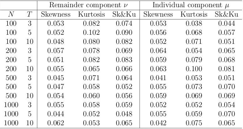
We explore the effectiveness of the proposed tests to alternative distributional processes. Table 1 reports experiments for ν ∼N(0,1) and µ∼ N(0,1). In this case, all tests should have empirical size close to 0.05. The results for the tests using bootstrap show very good empirical size for all different tests and panel sizes. In this case, tests for skewness in both

ν and µ have correct size for the smallest panel size considered (N = 100, T = 3). Tests for kurtosis start with oversized tests for N = 100 (0.07 to 0.10) but reduces to 0.05 as N

increases. Moreover, tests for joint skewness and kurtosis achieve correct empirical size as

N increases in a similar way to the tests for kurtosis.

[Table 1 about here]

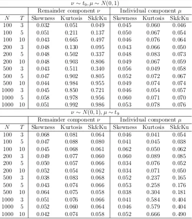
Table 2 reports experiments forν ∼t9, µ∼N(0,1) (first set of rows) andν ∼N(0,1), µ∼

t9 (second set of rows). Thet9-Student distribution is symmetric but presents excess kurtosis,

while the 9 degrees of freedom guarantees that all required moments are finite. In the first case, tests for kurtosis inν should have non trivial empirical power, while tests for skewness in ν and skewness and kurtosis in µ should not. In the second case, tests for kurtosis in µ

should have relevant power, while tests for skewness in µ and skewness and kurtosis in ν

should not. The experiments show that this is indeed the case. Forν ∼t9, µ ∼N(0,1), the

kurtosis test forν has power increasing in eitherN orT, while the remaining tests have size close to the 0.05 nominal size. For ν ∼ N(0,1), µ ∼ t9, the kurtosis test for µ has power

increasing only in N, while the remaining tests have size close to the 0.05 nominal size. The results show that kurtosis in one component does not affect tests for kurtosis in the other component.

[Table 2 about here]

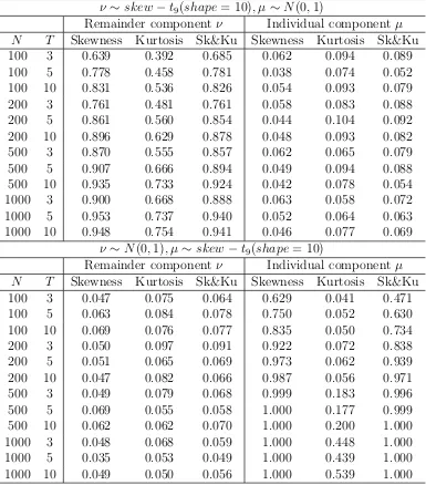
Tables 3 and 4 report experiments for skew normal distributions generated as in Azzalini (1985).1 _{The fact that skewness affects kurtosis implies that it is difficult to separate their}

effects in practice. To this purpose we consider Azzalini’s (1985) skew normal distribution with small skewness (as given by its shape parameter set to 1) and with minimum effect on the level of kurtosis; and next we consider a skew normal distribution with large skewness and, consequently, a large effect on kurtosis (shape parameter set to 10). Table 3 (shape set

1_{We are grateful to an anonymous referee for pointing this out. See Genton (2004) for a review of}

to 1) reveals that our proposed tests are able to detect departures from symmetry in each component without altering the empirical size in kurtosis. That is, tests for skewness in ν

have power increasing in either N or T and tests for skewness in µ have power increasing only inN when the corresponding component follows a skew normal distribution with shape 1. Moreover, the corresponding kurtosis tests have small power (the largest rejection rate is 0.128 for N = 1000, T = 10 in the ν test case and 0.075 for N = 200, T = 10 in the µ test case). Table 4 shows that a shape parameter of 10 affects the tests for both skewness and kurtosis. Overall, the results show that skewness (and kurtosis) in one component does not affect the tests for the other component.

[Table 3 about here]

[Table 4 about here]

Tables 5 and 6 reports experiments for skew t9-Student distributions generated as in

Azzalini and Capitanio (2003) with a shape parameter of 1 and 10.2 _{In this case we consider}

skewness and kurtosis together. The simulation results show that the developed tests are responsive to both deviations in skewness and kurtosis, and that deviations in one component does not affect the empirical size in the other component.

[Table 5 about here]

[Table 6 about here]

6

Empirical application: investment models

As an empirical illustration we apply the developed tests to the Fazzari, Hubbard and Pe-tersen (1988) investment equation model, where firm investment is regressed on a proxy for investment demand (Tobin’s q) and its cash flow; a widely used model in the corporate investment literature. Following Fazzari, Hubbard, and Petersen (1988), investment–cash-flow sensitivities became a standard metric in the literature that examines the impact of financing imperfections on corporate investment. These empirical sensitivities are also used

2_{We are grateful to an anonymous referee for pointing this out. Although not reported we also produced}

experiments withχ2

to draw inferences about efficiency in internal capital markets, the effect of agency on corpo-rate spending, the role of business groups in capital allocation, and the effect of managerial characteristics on corporate policies.

Tobin’s q is the ratio of the market valuation of a firm and the replacement value of its assets. Firms with a high value of q are considered attractive as investment opportunities, whereas a low value of q indicates the opposite. Investment theory is also interested in the effect of cash flow, as the theory predicts that financially constrained firms are more likely to rely on internal funds to finance investment (see Almeida, Campello and Galvao (2010), for a discussion). The baseline model in the literature is

Iit/Kit=α+βqit−1+γCFit−1/Kit−1+µi+νit,

whereIdenotes investment, K capital stock,CF cash flow,q Tobin’sq,µis the firm-specific effect andν is the innovation term.

We check for skewness and kurtosis in both µ and ν using the proposed tests. We are interested in testing for skewness and kurtosis for at least three reasons. First, testing normality plays a key role in forecasting models at the firm level. Second, asymmetry in both components is used for solving measurement error problems in Tobin’s q. The operationalization of q is not clear-cut, so estimation poses a measurement error problem. Many empirical investment studies found a very disappointing performance of theqtheory of investment, although this theory has a good performance when measurement error is purged as in Erickson and Whited (2000). Their method requires asymmetry in the error term to identify the effect of q on firm investment. Third, skewness and kurtosis by themselves provide information about the industry investment patterns. Skewness inµdetermines that a few firms either invest or disinvest considerably more than the rest, while kurtosis in µ

determine that a few firms locate at both sides of the investment line, that is, some invest a large amount while others disinvest large amounts too. Skewness and/or kurtosis in ν show that the large values of investment correspond to firm level shocks.

firm-years and 82 firms. Because we only consider firms that report information in each of the five years, the sample consists mainly of relatively large firms. We apply the proposed tests using B = 200 bootstrap repetitions.

The firm level componentµis found to be largely asymmetric (rejecting the null hypoth-esis Hsµ

0 : sµ = 0 of symmetry with a bootstrap p-value of 0.002) but with kurtosis close

to the normal value of 3 (cannot reject the null hypothesis Hkµ

0 : kµ = 3 with a bootstrap

p-value of 0.967). The joint test for the null hypothesis Hsµ&kµ

0 : sµ = 0 and kµ = 3 is also

rejected with a bootstrap p-value of 0.008. The remainder component ν shows both lack of symmetry (rejecting the null hypothesis Hsν

0 :sν = 0 of symmetry with a bootstrap p-value

of 0.002) and excess kurtosis (rejecting the null hypothesis Hkν

0 : kν = 3 with a bootstrap

p-value of 0.025), and a joint test forHsν&kν

0 :sν = 0 andkν = 3 with a bootstrapp-value of

0.001.

7

Conclusion and suggestions for future research

In this paper we have developed tests for skewness and/or for excess kurtosis for the one-way error components model. The tests are based on moment restrictions and are implemented after pooled OLS estimation. Besides being informative about non-Gaussian behavior, our tests can identify whether skewed errors and/or excess kurtosis arise in one or both com-ponents of the model, separately and jointly, hence providing useful information when non-normalities may affect the statistical properties of inferential strategies, and when detecting the possible presence of asymmetric or heavy tailed errors is a statistical and economic relevant question per se. The tests are implemented using the bootstrap method. The ex-periments show that empirical sizes are close to nominal ones for sample sizes similar to those used in empirical practice, and that the tests have very good power properties.

References

Almeida, H., Campello, M., and Galvao, A. (2010). “Measurement errors in investment equations,” Review of Financial Studies, 23, 3279–3328.

Azzalini, A. (1985). “A class of distributions which includes the normal ones,” Scandinavian Journal of Statistics, 12, 171-178.

Azzalini, A. and Capitanio, A. (2003). “Distributions generated by perturbation of symmetry with emphasis on a multivariate skew-t distribution,”Journal of the Royal Statistical Society Series B, 65, 367–389.

Bai, J. and Ng, S., (2005). “Tests for skewness, kurtosis, and normality for time series data,”

Journal of Business & Economic Statistics, 23, 49–60.

Baltagi, B.H., Bresson, G. and Pirotte, A., (2006). “Joint LM test for homoskedasticity in a one-way error component model,” Journal of Econometrics, 134, 401–417.

Baltagi, B.H., Song, S. H. and Koh, W., (2003). “Testing panel data regression models with spatial error correlation,” Journal of Econometrics, 68, 133–151.

Baltagi, B.H., Song, S.H., Jung, B.C. and W. Koh, (2007). “Testing for serial correlation, spatial autocorrelation and random effects using panel data,”Journal of Econometrics, 140, 5–51.

Bera, A. and Premaratne, G., (2001). “Adjusting the tests for skewness and kurtosis for distributional misspecifications,” working paper, University of Illinois at Urbana-Champaign,

http://www.business.uiuc.edu/Working_Papers/papers/01-0116.pdf

Blanchard, P. and M´aty´as, L., (1996). “Robustness of tests for error component models to non-normality,” Economics Letters, 51, 161–167.

Bontemps, C. and Meddahi, N., (2005). “Testing Normality: A GMM Approach,” Journal of Econometrics, 124, 149–186.

Dufour, J-M., Khalaf, L. and Beaulieu, M-C., (2003). “Exact skewness-kurtosis tests for multivariate normality and goodness-of-fit in multivariate regressions with application to asset pricing models,”Oxford Bulletin of Economics and Statistics, 65, 891– 906.

Ergun, A.T. and Jun, J., (2010). “Conditional skewness, kurtosis, and density specifica-tion testing: Moment-based versus nonparametric tests,” Studies in Nonlinear Dynamics & Econometrics, 14, Article 5.

Erickson, T. and Whited, T. M. (2000). “Measurement error and the relationship between investment and q,” Journal of Political Economy, 108, 1027–1057.

Evans, M., (1992). “Robustness of size of tests of autocorrelation and heteroskedasticity to nonnormality,”Journal of Econometrics, 51, 7–24.

Fazzari, S., R. G. Hubbard, and B. Petersen (1988). “Financing constraints and corporate investment,”Brooking Papers on Economic Activity,, 1, 141–195.

Genton, G. (2004). Skew-Elliptical Distributions and Their Applications. A Journey Beyond Normality, Chapman & Hall/CRC, London.

Gilbert, S., (2002). “Testing the distribution of error components in panel data models,”

Economics Letters, 77, 47–53.

Goncalves, S. (2011). “The moving blocks bootstrap for panel linear regression models with individual fixed effects,” Econometric Theory, 27, 1048–1082.

Henze, N. (1994). “On Mardias kurtosis test for multivariate normality,” Communications in Statistics, Part A - Theory and Methods, 23, pp. 1031–1045.

Holly, A. and Gardiol, L., (2000). “A score test for individual heteroskedasticity in a one-way error components model,” In: Krishnakumar, J., Ronchetti, E. (Eds.), Panel Data Econometrics: Future Directions, Elsevier, Amsterdam, pp. 199–211.

Jarque, C.M. and Bera, A.K., (1981). “Efficient tests for normality, homoscedasticity and serial independence of regression residuals: Monte Carlo evidence,”. Economics Letters, 7, 313–318.

kurto-sis,”. The American Statistician, 65, 89–95.

Kapetanios, G. (2008). “A bootstrap procedure for panel datasets with many cross-sectional units,” Econometrics Journal, 11, 377–395.

Lutkepohl, H. and Theilen, B. (1991). “Measures of multivariate skewness and kurtosis for tests of nonnormality,” Statistical Papers, 32, 179–193.

Meintanis, S.G., (2011). “Testing for normality with panel data,” Journal of Statistical Computation and Simulation, 81, 1745–1752.

Montes-Rojas, G. and Sosa-Escudero, W., (2011). “Robust tests for heteroskedasticity in the one-way error components model,”Journal of Econometrics, 160, 300–310.

Pesaran, M. H. and Tosetti, E., (2009). “Large panels with spatial correlation and common factors,” Working Paper.

Premaratne, G. and Bera, A., (2005), “A test for symmetry with leptokurtic financial data,”

Journal of Financial Econometrics, 3, 169–187.

Shao, J. and Tu, D., (1995). The Jackknife and Bootstrap, Springer-Verlag, New York, New York.

Appendix A

A1. Variance

We present estimators of the variance of µand ν. First, we derive some equalities based on which we estimate the variance of µ and ν. Note that u2_i = (µi +νi)2 = µ2i +ν2i + 2µiνi.

Taking expectation, we have

E[u2_i] =σ_µ2+T−1σ2_ν.

The square of the within residuals is given by u_e2_it = (uit−ui)2 =νit2 +ν2i −2νitνi, and after

taking expectations

E[u_e2_it] =σ_ν2+T−1σ_ν2−2T−1σ2_ν =σ_ν2 1−T−1.

Solving these equations for σ2

µ and σν2, we obtain

σ2_ν = 1

1−T−1E[eu

2

i] =

1

1−T−1E[u 2

i]−

1

1−T−1E[u 2

i],

σ_µ2 = E[u2_i]− 1

T −1E[eu

2

i] = E[u

2

i]−

1

T −1E[u

2

i −u

2

i] =

T T −1E[u

2

i]−

1

T −1E[u

2

i].

Next, given this derivation, we consider the following statistics that are the sample coun-terpart of the above expressions, respectively, by replacing the theoretical with the sample expectations and using _buit, the OLS residuals

b

σ_ν2 = 1

1−T−1E[ub

2

i]−

1

1−T−1E[ub

2

i] =

1

1−T−1E[u 2

i]−

1

1−T−1E[u 2

i] +op(N−1/2),

b

σ_µ2 = T

T −1E[ub

2

i]−

1

T −1E[bu

2

i] =

T T −1E[u

2

i]−

1

T −1E[u

2

i] +op(N−1/2).

The second equalities of the two lines above follows from Lemmas 1 and 2 (in Appendix B) with j = 2. Therefore,

√

N(σ_bν2−σ_ν2) =A1

1

√

N

N

X

i=1

Ai+op(1),

√

N(_bσ_µ2−σ_µ2) =A2

1

√

N

N

X

i=1

and by delta method and Slutsky’s lemma, respectively,

√

N(_bσ_ν4−σ4_ν) = 2σ2_νA1

1 √ N N X i=1

Ai+op(1),

√

N(_bσ_µ2σ_bν2−σ_µ2σ_ν2) = (σ_µ2A1+σ2νA2)

1 √ N N X i=1

Ai+op(1).

A2. Proof of Theorem 1

A2.1 Proof of skewness results in (i) and (ii)

Note that

√

N(SKd_ν−s_ν) =

√ N b ν3 b σ3 ν − ν3

σ3

ν

=√N

b

ν3−ν3

b

σ3

ν

−3sνσν(bσ

2

ν −σ2ν)

2_bσ3

ν

+op(1), √

N(SK[µ−sµ) = √ N b µ3 b σ3 µ − µ3

σ3

µ

=√N

b

µ3−µ3

b

σ3

µ

− 3sµσµ(σb

2

µ−σ2µ)

2_bσ3

µ

+op(1).

Then we only need to find asymptotic linear representations of√N(_bν3−ν3) and

√

N(µ_b3−µ3),

since those of √N(σ_bν2 −σ_ν2) and √N(σ_bµ2 −σ_µ2) are obtained in Appendix A1. Using the conclusions of Lemmas 1 and 2 (in Appendix B) for j = 3 and the first equality of Lemma 3 (in Appendix B), we have

√

N(ν_b3−ν3) =

√

N

1

1−3T−1_{+ 2T}−2E[bu

3

i −3buibu

2

i + 2ub

3

i]−ν3

= 1

1−3T−1 _{+ 2T}−2

" 1 √ N N X i=1 u3 i − √

NE[u3

i]−3E[u

2 it] 1 √ N N X i=1 ui !

−3 √1

N

N

X

i=1

u2_iui− √

NE[u2_iui]−

1 √ N N X i=1

uiE[u2it+ 2u

2

i]

!

+2 √1

N

N

X

i=1

u3_i −√NE[u_i3]−3E[u2_i]√1

N N X i=1 ui !#

+op(1)

=

1 √

N

PN

i=1u 3

i − √

NE[u3

i]−3√1_N

PN

i=1u 2

iui+ 3 √

NE[u2

iui] + 2√1_N PN_i=1u3i −2 √

NE[u3

i]

1−3T−1_{+ 2T}−2 +op(1)

=B1

1 √ N N X i=1

√

N(µ_b3−µ3) =

√

N

T2_−3T

T2_{−3T + 2}E[ub

3

i]−

1

T2_{−3T + 2}E[ub

3

i −3ubiub

2

i]−µ3

= T

2 _−3T

T2_{−3T + 2}

1 √ N N X i=1

u3_i −√NE[u_i3]−3E[u2_i]√1

N N X i=1 ui ! − 1

T2_{−3T + 2}

1 √ N N X i=1 u3 i − √

NE[u3

i]−3E[u

2 it] 1 √ N N X i=1 ui !

+ 3 √1

N

N

X

i=1

u2

iui− √

NE[u2

iui]−

1 √ N N X i=1

uiE[u2it+ 2u

2

i]

!

÷(T2−3T + 2) +op(1)

= T

2 _−3T

T2_{−3T + 2}

1 √ N N X i=1

u3_i −√NE[u3_i]

!

− 1

T2_{−3T + 2}

1 √ N N X i=1 u3 i − √

NE[u3

i]

!

+ 3

T2_{−3T + 2}

1 √ N N X i=1 u2

iui− √

NE[u2

iui]

!

−3E[u2_i]√1

N

N

X

i=1

ui+op(1)

=B2

1 √ N N X i=1

Ai+op(1).

Therefore,

√

N(SKd_ν −s_ν) = _B

1

σ3

ν

−3sνA1

2σ2

ν 1 √ N N X i=1

Ai+op(1)

√

N(SK[µ−sµ) =

_B

2

σ3

µ

− 3sµA2

2σ2

µ 1 √ N N X i=1

Ai+op(1).

A2.2 Proof of kurtosis results in (iii) and (iv)

Note that

√

N(KU[ν−kν) = √ N b ν4 b σ4 ν − ν4

σ4

ν

=√N

b

ν4−ν4

b

σ4

ν

− 2kνσ

2

ν(σb

2

ν −σν2)

b

σ4

ν

+op(1), √

N(KU[µ−kµ) = √ N b µ4 b σ4 µ − µ4

σ4

µ

=√N

b

µ4−µ4

b

σ4

µ

−2kµσ

2

µ(bσ

2

µ−σµ2)

b

σ4

µ

+op(1).

Then we only need to find asymptotic linear representations of√N(_bν4−ν4) and

√

N(µ_b4−µ4),

since those of √N(σ_b2

ν −σν2) and √

N(σ_b2

µ −σµ2) are obtained in Appendix A1. Using the

Lemma 3 (in Appendix B),

√

N(ν_b4−ν4) =

√

N E[bu

4

i]−4E[ub

3

iubi] + 6E[bu

2

ibu

2

i]−3E[ub

4

i]

1−4T−1_{+ 6T}−2_−3T−3 −

(T −1)(6T−2−12T−3) 1−4T−1_{+ 6T}−2_−3T−3σb

4

ν −ν4

! = " 1 √ N N X i=1 1 T T X t=1

u4_it−√NE[u4

i]−4E[u

3 it] 1 √ N N X i=1 ui !

−4 √1

N

N

X

i=1

u3

iui− √

NE[u3

iui]−E[3u2iui+u3it]

1 √ N N X i=1 ui !

+ 6 √1

N N X i=1 u2 iu 2 i − √

NE[u2

iu

2

i]−2E[u

3

i +u2iui]

1 √ N N X i=1 ui !

−3 √1

N

N

X

i=1

u4_i −√NE[u_i4]−4E[u3_i]√1

N N X i=1 ui !#

÷(1−4T−1+ 6T−2−3T−3)

− (T −1)(6T

−2_−12T−3₎

1−4T−1_{+ 6T}−2 _−3T−32σ 2

νA1

1 √ N N X i=1

Ai+op(1)

=C1

1 √ N N X i=1

Ai+op(1),

√

N(µ_b4−µ4) =

√

N _E[_bu4_i] T

3_−4T2_{+ 6T}

T3_−4T2_{+ 6T −3} −

E[ub

4

i]−4E[bu

3

ibui] + 6E[bu

2

iub

2

i]

T3_−4T2_{+ 6T −3}

−(T −1)(3T

3_−12T2_{+ 12T + 3)}

(T3_−4T2_{+ 6T −3)T}3 bσ

4

ν −

6

Tbσ

2

µσb

2

ν −µ4

= T

3 _−4T2_{+ 6T}

T3_−4T2_{+ 6T −3}

1 √ N N X i=1

u4_i −√NE[u_i4]−4E[u3_i]√1

N N X i=1 ui ! − 1

T3_−4T2_{+ 6T −3}

1 √ N N X i=1 u4 i − √

NE[u4

i]−4E[u

3 it] 1 √ N N X i=1 ui ! + 4

T3_−4T2_{+ 6T −3}

1 √ N N X i=1 u3

iui− √

NE[u3

iui]−

1 √ N N X i=1

uiE[3u2iui+u3it]

!

− 6

T3_−4T2_{+ 6T −3}

1 √ N N X i=1 u2 iu 2 i − √

NE[u2

iu

2

i]−2

1 √ N N X i=1

uiE[u3i +u2iui]

!

−(T −1)(3T

3_−12T2_{+ 12T + 3)}

(T3 _−4T2_{+ 6T −3)T}3 2σ 2

νA1

1 √ N N X i=1 Ai ! − 6

T (σ

2

µA1+σν2A2)

1 √ N N X i=1 Ai !

+op(1)

=C2

1 √ N N X i=1

Therefore,

√

N(KU[ν −kν) =

C1

σ4

ν

−2kνA1

σ2 ν 1 √ N N X i=1

Ai+op(1)

√

N(KU[µ−kµ) =

C2

σ4

µ

− 2kµA2

σ2 µ 1 √ N N X i=1

Ai+op(1).

A3. Proof of Theorem 2

We prove the conclusion (i) only because the conclusions of the other three are similar. By Lindeberg-L´evy central limit theorem and Assumption 1, √1

N

PN

i=1Ai converges to a

normal distribution. Then, using the continuous mapping theorem,B1

σ3

ν − 3sνA1

2σ2

ν 1 √ N PN

i=1Ai

converges to a normal distribution with mean zero and variance-covariance matrix denoted by Ωs_ν. Applying the continuous mapping theorem again, we obtain (i).

A4. Proof of Proposition 1

We will prove only the consistency of the bootstrap estimator of Ωs

ν as the the consistency of

the other estimators are similar. We apply Theorem 3.8 of Shao and Tu (1995) as the statistic is an average_EhB1

σ3

ν − 3sνA1

2σ2

ν

Bi

i

, where_Bi = (ui, u2i, u2i, u3i, u3i, ui4, u4i, u2iui, u3iui, u2iu2i)

>_{. We}

focus on verifying condition (3.28). It suffices to show that

max1≤i≤N

B1 σ3 ν − 3sνA1

2σ2

ν

Bi−E

h

B1

σ3

ν − 3sνA1

2σ2

ν Bi i τN a.s. → 0,

which is implied by Assumption 3.

Appendix B

Auxiliary Lemmas

In this appendix we list some results that are useful for the proofs of the theorems.

Lemma 1 Under Assumptions 1 and 2, for j =2, 3, and 4, we have

1 √ N N X i=1 b

uj_i = √1

N

N

X

i=1

uj_i −jE[uj_it−1]√1

N

N

X

i=1

Proof. The proof is complete if the following equalities hold. 1 √ N N X i=1 1 T T X t=1 b

uj_it=√1

N N X i=1 1 T T X t=1

(uit−u)j+op(1),

1 √ N N X i=1 1 T T X t=1

(uit−u)j =

1 √ N N X i=1 1 T T X t=1

uj_it−jE[uj_it−1]√1

N N X i=1 1 T T X t=1

uit+op(1).

The proofs of the first and second equalities are modifications of the proofs of Theorem 5 and Lemma A.1., respectively, of Bai and Ng (2005) to accommodate the one-way error components panel data model.

Lemma 2 Under Assumptions 1 and 2, for j =2, 3, and 4, we have

1 √ N N X i=1 b

uj_i = √1

N

N

X

i=1

uj_i −jE[uj_i−1]√1

N

N

X

i=1

ui+op(1).

Proof. Noting that _buit = (uit−u)−(xit−x)>(βb−β₀), we have b

ui = (ui −u)−(xi −

x)>(βb−β0). Also, we will use the fact that βb−β0 =Op(N−1/2) and that

1 √ N N X i=1

(ui−u)a

(xi−x)>(βb−β₀) b

=Op(N−1/2)

wherea≥0 andb >0 are integers. In fact, whenevera≥0 andb≥2, if E[(ui−u)a||xi−x||b]

exists, the expression equals

Op(N1/2)Op(N−b/2) =Op(N(1−b)/2) =Op(N−1/2).

When a≥0 and b= 1, 1 √ N N X i=1

(ui−u)a(xi−x)>(βb−β0)

=√1

N

N

X

i=1

((ui−u)a−E[(ui−u)a])(xi−x)>(βb−β0) =Op(1)Op(N−1/2).

For j = 2, 1 √ N N X i=1 b

u2_i = √1

N

N

X

i=1

(ui−u)−(xi−x)>(βb−β₀) 2

=√1

N

N

X

i=1

(ui−u)2+

1 √ N N X i=1

(xi−x)>(βb−β₀) 2

−2√1

N

N

X

i=1

(ui−u)

(xi−x)>(βb−β₀)

=√1

N

N

X

i=1

u2_i +u2−2uiu

+Op(N1/2)Op(N−1)−Op(1)Op(N−1/2) =

1 √ N N X i=1

For j = 3, 1 √ N N X i=1 b

u3_i = √1

N

N

X

i=1

(ui−u)−(xi−x)>(βb−β₀) 3

=√1

N

N

X

i=1

(ui−u)3−

1 √ N N X i=1

(xi−x)>(βb−β₀) 3

−3√1

N

N

X

i=1

(ui−u)2

(xi−x)>(βb−β₀)

+ 3√1

N

N

X

i=1

(ui−u)

(xi−x)>(βb−β₀) 2

=√1

N

N

X

i=1

u3_i −u3−3u2_iu+ 3uiu2

−Op(N1/2)Op(N−3/2)−Op(1)Op(N−1/2) +Op(1)Op(N−1)

=√1

N

N

X

i=1

u3_i −3(σ2_µ+T−1σ_ν2)√1

N

N

X

i=1

ui+op(1).

For j = 4,

1 √ N N X i=1 b

u4_i = √1

N

N

X

i=1

(ui−u)−(xi−x)>(βb−β₀) 4

=√1

N

N

X

i=1

(ui−u)4+

1 √ N N X i=1

(xi−x)>(βb−β₀) 4

−4√1

N

N

X

i=1

(ui−u)3

(xi−x)>(βb−β₀)

−4√1

N

N

X

i=1

(ui −u)

(xi−x)>(βb−β₀) 3

+ 6√1

N

N

X

i=1

(ui−u)2

(xi −x)>(βb−β₀) 2

=√1

N

N

X

i=1

u4_i +u4−4u3_iu−4uiu3 + 6u2iu

2

+Op(N−1/2)

=√1

N

N

X

i=1

u4_i −4(µ3+T−2ν3)

1 √ N N X i=1

ui +op(1).

Lemma 3 Under Assumptions 1 and 2, the following equalities hold.

(i) √1

N N X i=1 b u2

iubi =

1 √ N N X i=1 u2

iui− √

N uE[u2_it+ 2u2_i] +op(1)

(ii) √1

N N X i=1 b u3

iubi =

1 √ N N X i=1 u3

iui− √

N uE[3u2

iui+u3it] +op(1)

(iii) √1

N N X i=1 b u2

iub

2 i = 1 √ N N X i=1 u2 iu 2

i −2 √

N uE[u3_i +u2

Proof. To derive the first equality, we conduct the following calculations. 1 √ N N X i=1 b u2

iubi =

1 √ N N X i=1

[(ui−u)−(xi−x)>(βb−β₀)]2×[(u_i−u)−(x_i−x)>(βb−β₀)]

=√1

N

N

X

i=1

[(ui−u)2 −2(ui−u)(xi−x)>(βb−β₀) + [(x_i−x)>(βb−β₀)]2][(u_i−u)−(x_i−x)>(βb−β₀)]

=√1

N

N

X

i=1

[(u2

i −2uiu+u2)−2(ui−u)(xi−x)>(βb−β₀) +O_p(N−1)][(u_i−u)−(x_i−x)>(βb−β₀)]

=√1

N

N

X

i=1

(u2

i −2uiu+u2)(ui−u)−2(ui−u)(ui−u)(xi−x)>(βb−β₀)

−(u2

i −2uiu+u2)(xi−x)>(βb−β₀) +o_p(1)

=√1

N

N

X

i=1

u2

iui− √

N uE[u2_it+ 2u2_i]−2√N(βb−β₀)>(E[u_iu_ix_i]−E[u2_ix]) +o_p(1)

=√1

N

N

X

i=1

u2

iui− √

N uE[u2_it+ 2u2_i] +op(1).

Now we establish the second equality.

1 √ N N X i=1 b u3

iubi =

1 √ N N X i=1

[(ui−u)−(xi−x)>(βb−β₀)]3 ×[(u_i−u)−(x_i−x)>(βb−β₀)]

=√1

N

N

X

i=1

[(ui−u)3−3(ui−u)2(xi−x)>(βb−β₀) + 3(u_i−u)[(x_i−x)>(βb−β₀)]2

−[(xi−x)>(βb−β₀)]3][(u_i−u)−(x_i−x)>(βb−β0)]

=√1

N

N

X

i=1

[(u3_i −3u2_i u+ 3uiu2−u3)−3(u2i −2uiu+u2)(xi−x)>(βb−β0) +Op(N−1)]

×[(ui −u)−(xi−x)>(βb−β₀)]

=√1

N

N

X

i=1

(u3

i −3u2i u+ 3uiu2−u3)(ui−u)−3(ui−u)(u2i −2uiu+u2)(xi−x)>(βb−β0)

−(u3

i −3u2i u+ 3uiu2−u3)(xi −x)>(βb−β₀) +o_p(1)

=√1

N

N

X

i=1

u3

iui− √

N uE[3u2

iui+u3it]−2 √

N(βb−β0)>(E[uiu2ixi]−E[uiu2ix]) +op(1)

=√1

N

N

X

i=1

u3

iui− √

N uE[3u2

Finally, we show the third equality.

1

√

N

N

X

i=1

b

u2

iub

2

i =

1

√

N

N

X

i=1

[(ui−u)−(xi−x)>(βb−β₀)]2×[(u_i−u)−(x_i−x)>(βb−β₀)]

2

=√1

N

N

X

i=1

[(ui−u)2 −2(ui−u)(xi−x)>(βb−β₀) + [(x_i−x)>(βb−β₀)]2]

×[(ui−u)2−2(ui−u)(xi−x)>(βb−β₀) + [(x_i−x)>(βb−β₀)]2]

=√1

N

N

X

i=1

[(u2

i −2uiu+u2)−2(ui−u)(xi−x)>(βb−β₀) +O_p(N−1)]

×[(u2_i −2uiu+u2)−2(ui−u)(xi−x)>(βb−β₀) +O_p(T−1)]

=√1

N

N

X

i=1

(u2

i −2uiu+u2)(u2i −2uiu+u2)−(u2i −2uiu+u2)2(ui−u)(xi−x)>(βb−β₀)

(u2

i −2uiu+u2)2(ui−u)(xi−x)>(βb−β₀) +o_p(1)

=√1

N

N

X

i=1

u2

iu

2

i −2 √

N uE[u3_i +u2

iui] + 2 √

N(βb−β₀)>E[u3_ix−u2_iu_ix_i] +o_p(1)

=√1

N

N

X

i=1

u2

iu

2

i −2 √

N uE[u3_i +u2

Table 1: ν ∼N(0,1), µ ∼N(0,1)

Remainder component ν Individual component µ N T Skewness Kurtosis Sk&Ku Skewness Kurtosis Sk&Ku 100 3 0.053 0.082 0.074 0.053 0.038 0.044 100 5 0.052 0.102 0.090 0.056 0.068 0.057 100 10 0.048 0.080 0.082 0.052 0.071 0.051 200 3 0.057 0.078 0.069 0.064 0.054 0.065 200 5 0.051 0.082 0.083 0.059 0.079 0.068 200 10 0.055 0.065 0.066 0.063 0.100 0.081 500 3 0.045 0.071 0.064 0.041 0.053 0.051 500 5 0.047 0.058 0.052 0.055 0.073 0.070 500 10 0.054 0.060 0.056 0.059 0.069 0.069 1000 3 0.055 0.058 0.059 0.052 0.052 0.054 1000 5 0.044 0.052 0.048 0.055 0.059 0.070 1000 10 0.062 0.053 0.065 0.042 0.075 0.065

Table 2: ν ∼t9, µ ∼N(0,1) and ν ∼N(0,1), µ∼t9

ν∼t9, µ∼N(0,1)

Remainder component ν Individual component µ N T Skewness Kurtosis Sk&Ku Skewness Kurtosis Sk&Ku 100 3 0.032 0.051 0.049 0.045 0.060 0.046 100 5 0.051 0.211 0.137 0.050 0.067 0.054 100 10 0.043 0.665 0.497 0.046 0.076 0.064 200 3 0.048 0.130 0.095 0.043 0.066 0.050 200 5 0.048 0.502 0.337 0.048 0.083 0.073 200 10 0.048 0.903 0.806 0.049 0.067 0.059 500 3 0.043 0.511 0.340 0.056 0.049 0.058 500 5 0.047 0.902 0.805 0.052 0.072 0.067 500 10 0.044 0.984 0.955 0.049 0.074 0.074 1000 3 0.045 0.850 0.721 0.046 0.054 0.057 1000 5 0.058 0.978 0.956 0.060 0.071 0.070 1000 10 0.051 0.992 0.986 0.053 0.078 0.076

ν∼N(0,1), µ ∼t9

Remainder component ν Individual component µ N T Skewness Kurtosis Sk&Ku Skewness Kurtosis Sk&Ku 100 3 0.068 0.081 0.064 0.046 0.041 0.054 100 5 0.047 0.088 0.080 0.041 0.045 0.038 100 10 0.045 0.068 0.061 0.062 0.050 0.062 200 3 0.049 0.077 0.060 0.060 0.089 0.085 200 5 0.050 0.057 0.066 0.034 0.076 0.052 200 10 0.052 0.054 0.062 0.034 0.071 0.050 500 3 0.038 0.083 0.068 0.052 0.237 0.165 500 5 0.043 0.074 0.066 0.053 0.258 0.176 500 10 0.064 0.075 0.058 0.038 0.304 0.181 1000 3 0.051 0.076 0.066 0.041 0.584 0.404 1000 5 0.052 0.060 0.064 0.046 0.579 0.404 1000 10 0.042 0.074 0.058 0.052 0.666 0.490

Table 3: ν ∼ skew − normal(shape = 1), µ ∼ N(0,1) and ν ∼ N(0,1), µ ∼ skew −

normal(shape= 1)

ν ∼skew−normal(shape= 1), µ∼N(0,1)

Remainder component ν Individual component µ N T Skewness Kurtosis Sk&Ku Skewness Kurtosis Sk&Ku 100 3 0.058 0.087 0.088 0.049 0.057 0.045 100 5 0.138 0.061 0.112 0.040 0.071 0.062 100 10 0.324 0.055 0.237 0.059 0.056 0.053 200 3 0.081 0.080 0.095 0.041 0.053 0.043 200 5 0.214 0.046 0.161 0.047 0.082 0.060 200 10 0.534 0.046 0.442 0.053 0.093 0.074 500 3 0.160 0.069 0.133 0.059 0.050 0.049 500 5 0.490 0.054 0.393 0.050 0.069 0.060 500 10 0.915 0.054 0.839 0.048 0.085 0.074 1000 3 0.294 0.049 0.218 0.049 0.059 0.053 1000 5 0.779 0.056 0.690 0.055 0.060 0.058 1000 10 0.997 0.128 0.993 0.052 0.076 0.065

ν ∼N(0,1), µ∼skew−normal(shape= 1)

Remainder component ν Individual component µ N T Skewness Kurtosis Sk&Ku Skewness Kurtosis Sk&Ku 100 3 0.052 0.091 0.083 0.063 0.046 0.048 100 5 0.054 0.072 0.065 0.078 0.063 0.063 100 10 0.040 0.078 0.065 0.069 0.059 0.061 200 3 0.050 0.077 0.076 0.084 0.054 0.063 200 5 0.052 0.083 0.073 0.090 0.064 0.089 200 10 0.057 0.053 0.060 0.077 0.075 0.077 500 3 0.046 0.070 0.063 0.106 0.046 0.086 500 5 0.062 0.054 0.052 0.144 0.067 0.131 500 10 0.056 0.066 0.067 0.168 0.055 0.135 1000 3 0.049 0.072 0.064 0.171 0.055 0.146 1000 5 0.053 0.068 0.075 0.260 0.065 0.209 1000 10 0.048 0.047 0.051 0.328 0.042 0.260

Table 4: ν ∼ skew −normal(shape = 10), µ ∼ N(0,1) and ν ∼ N(0,1), µ ∼ skew −

normal(shape= 10)

ν ∼skew−normal(shape= 10), µ ∼N(0,1)

Remainder component ν Individual component µ N T Skewness Kurtosis Sk&Ku Skewness Kurtosis Sk&Ku 100 3 0.780 0.069 0.673 0.051 0.063 0.050 100 5 0.999 0.193 0.999 0.055 0.073 0.062 100 10 1.000 0.506 1.000 0.048 0.060 0.046 200 3 0.967 0.178 0.960 0.058 0.060 0.058 200 5 1.000 0.422 1.000 0.043 0.066 0.067 200 10 1.000 0.885 1.000 0.042 0.090 0.077 500 3 1.000 0.527 1.000 0.059 0.059 0.066 500 5 1.000 0.908 1.000 0.058 0.079 0.078 500 10 1.000 0.997 1.000 0.049 0.078 0.069 1000 3 1.000 0.901 1.000 0.058 0.057 0.059 1000 5 1.000 0.999 1.000 0.064 0.066 0.068 1000 10 1.000 1.000 1.000 0.050 0.062 0.069

ν ∼N(0,1), µ ∼skew−normal(shape= 10)

Remainder component ν Individual component µ N T Skewness Kurtosis Sk&Ku Skewness Kurtosis Sk&Ku 100 3 0.052 0.092 0.080 0.596 0.036 0.464 100 5 0.051 0.073 0.065 0.761 0.044 0.616 100 10 0.041 0.079 0.063 0.855 0.049 0.733 200 3 0.054 0.072 0.073 0.917 0.065 0.836 200 5 0.051 0.082 0.070 0.971 0.057 0.914 200 10 0.058 0.056 0.060 0.993 0.078 0.968 500 3 0.046 0.068 0.062 1.000 0.154 0.999 500 5 0.061 0.053 0.051 0.999 0.182 0.998 500 10 0.058 0.067 0.066 1.000 0.217 1.000 1000 3 0.050 0.070 0.066 1.000 0.433 1.000 1000 5 0.054 0.068 0.074 1.000 0.458 1.000 1000 10 0.049 0.048 0.051 1.000 0.506 1.000

Table 5: ν∼skew−t9(shape= 1), µ ∼N(0,1) and ν ∼N(0,1), µ∼skew−t9(shape= 1)

ν ∼skew−t9(shape= 1), µ∼N(0,1)

Remainder component ν Individual component µ N T Skewness Kurtosis Sk&Ku Skewness Kurtosis Sk&Ku 100 3 0.287 0.339 0.475 0.060 0.081 0.069 100 5 0.509 0.478 0.645 0.049 0.064 0.058 100 10 0.713 0.623 0.779 0.049 0.085 0.066 200 3 0.496 0.516 0.660 0.048 0.072 0.066 200 5 0.716 0.630 0.779 0.047 0.088 0.079 200 10 0.805 0.664 0.836 0.059 0.081 0.074 500 3 0.744 0.646 0.803 0.054 0.070 0.070 500 5 0.832 0.667 0.847 0.064 0.085 0.083 500 10 0.903 0.752 0.904 0.048 0.081 0.061 1000 3 0.828 0.686 0.844 0.061 0.039 0.058 1000 5 0.909 0.763 0.913 0.046 0.059 0.062 1000 10 0.926 0.785 0.924 0.047 0.073 0.063

ν ∼N(0,1), µ∼skew−t9(shape= 1)

Remainder component ν Individual component µ N T Skewness Kurtosis Sk&Ku Skewness Kurtosis Sk&Ku 100 3 0.038 0.075 0.055 0.190 0.171 0.271 100 5 0.047 0.085 0.074 0.163 0.169 0.261 100 10 0.048 0.062 0.058 0.206 0.221 0.316 200 3 0.043 0.071 0.050 0.295 0.294 0.441 200 5 0.061 0.077 0.075 0.292 0.318 0.448 200 10 0.056 0.059 0.056 0.338 0.346 0.487 500 3 0.041 0.079 0.064 0.511 0.491 0.650 500 5 0.053 0.045 0.046 0.520 0.490 0.648 500 10 0.042 0.055 0.048 0.546 0.534 0.677 1000 3 0.052 0.067 0.072 0.695 0.591 0.785 1000 5 0.045 0.052 0.054 0.691 0.573 0.763 1000 10 0.062 0.065 0.066 0.686 0.605 0.774