Measurement, modeling and perception of painted surfaces : A Multi-scale analysis of the touch-up problem

Rochester Institute of Technology

RIT Scholar Works

Theses Thesis/Dissertation Collections

2-1-2011

Measurement, modeling and perception of painted

surfaces : A Multi-scale analysis of the touch-up

problem

Suparna Kalghatgi

Follow this and additional works at:http://scholarworks.rit.edu/theses

This Thesis is brought to you for free and open access by the Thesis/Dissertation Collections at RIT Scholar Works. It has been accepted for inclusion in Theses by an authorized administrator of RIT Scholar Works. For more information, please [email protected].

Recommended Citation

Rochester Institute of Technology

MEASUREMENT, MODELING AND PERCEPTION OF

PAINTED SURFACES :

A Multi-scale Analysis of the Touch-up

Problem

A Thesis

Submitted in Partial Fulfillment of the

Master of Science in Industrial Engineering

in the

Department of Industrial & Systems Engineering

Kate Gleason College of Engineering

By

Suparna Kishore Kalghatgi

ii DEPARTMENT OF INDUSTRIAL & SYSTEMS ENGINEERING

KATE GLEASON COLLEGE OF ENGINEERING

ROCHESTER INSTITUTE OF TECHNOLOGY

ROCHESTER, NEW YORK

CERTIFICATE OF APPROVAL

M.S. DEGREE THESIS

The M.S. Degree Thesis of Suparna Kishore Kalghatgi

has been examined and approved by the

Thesis Committee as satisfactory for the

Thesis requirement for the

Master of Science degree

Approved by:

___________________________

Dr. Marcos Esterman, Thesis Advisor

___________________________

Dr. James A. Ferwerda

___________________________

iii

ACKNOWLEDGEMENTS

I would like to express my heartfelt gratitude towards my entire thesis committee- Dr. James A.

Ferwerda for his guidance, teaching and encouragement throughout the course of this thesis; Dr.

Marcos Esterman for his words of advice; and Dr. Matthew Marshall for his recommendations

and valuable suggestions.

I am thankful to Dr. Jonathan Arney, Dr. Susan Farnand and Dr. David R. Wyble, for their help

with the BRDF and surface topography measurements; and Dr. Koichi Takase, Dr. Tongbo Chen

and Lawrence Taplin, for their assistance in developing the code for normal map estimation.

My fellow members of the 3D Imaging Group at the Munsell Color Science Lab - Benjamin

Darling, Dan Zhang and Jonathan Phillips, have played a very significant role towards the

successful completion of this project. I thank them for their immense contribution in developing

the code used for the modeling and rendering of the synthetic images and for the psychophysical

experiments.

I would like to gratefully acknowledge Sherwin Williams Paints for funding this project, and our

company advisors- Paul H. Kayima, Shermila B. Singham and Mary E. Tuel for their invaluable

input at every stage of this research.

Lastly, I would like to recognize my parents- Kishore and Alka Kalghatgi, and my sister Pallavi.

It is their unconditional love, support and faith in me that has enabled me to complete my

Masters program successfully. I dedicate this thesis to them.

iv

ABSTRACT

Real-world surfaces typically have geometric features at a range of spatial scales. At the

microscale, opaque surfaces are often characterized by bidirectional reflectance distribution

functions (BRDF), which describes how a surface scatters incident light. At the mesoscale,

surfaces often exhibit visible texture – stochastic or patterned arrangements of geometric features

that provide visual information about surface properties such as roughness, smoothness, softness,

etc. These textures also affect how light is scattered by the surface, but the effects are at a

different spatial scale than those captured by the BRDF. Through this research, we investigate

how microscale and mesoscale surface properties interact to contribute to overall surface

appearance. This behavior is also the cause of the well-known “touch-up problem” in the paint

industry, where two regions coated with exactly the same paint, look different in color, gloss

and/or texture because of differences in application methods.

At first, samples were created by applying latex paint to standard wallboard surfaces. Two

application methods- spraying and rolling were used. The BRDF and texture properties of the

samples were measured, which revealed differences at both the microscale and mesoscale. This

data was then used as input for a physically-based image synthesis algorithm, to generate

realistic images of the surfaces under different viewing conditions. In order to understand the

factors that govern touch-up visibility, psychophysical tests were conducted using calibrated,

digital photographs of the samples as stimuli. Images were presented in pairs and a two

alternative forced choice design was used for the experiments. These judgments were then used

as data for a Thurstonian scaling analysis to produce psychophysical scales of visibility, which

helped determine the effect of paint formulation, application methods, and viewing and

illumination conditions on the touch-up problem. The results can be used as base data towards

development of a psychophysical model that relates physical differences in paint formulation and

v

TABLE OF CONTENTS

ABSTRACT iv

TABLE OF CONTENTS v

LIST OF FIGURES vii

LIST OF TABLES ix

1 MOTIVATION 1

2 BACKGROUND 3

2.1 PAINT 4

2.1.1 Paint formulation 4

2.1.2 Paint Application 5

2.1.3 Relationship between paint application effects and spatial scales 5

2.2 MEASUREMENT OF REFLECTANCE AND TEXTURE 7

2.2.1 Surface Reflectance Measurement 7

2.2.2 Measurement of Surface Topography 11

2.3 SURFACE MODELING AND RENDERING 14

2.3.1 Light Reflection Models 14

2.3.1.1 Empirical Models 15

2.3.1.2 Physically Based Models 16

2.3.2 Rendering 17

2.3.2.1 Rasterization 17

2.3.2.2 Ray Casting 17

2.3.2.3 Ray Tracing 18

2.3.2.4 Radiosity 18

2.3.3 Imaging 19

2.4 PSYCHOPHYSICS 21

2.4.1 Determination of Thresholds 21

2.4.2 Psychophysical Scaling 22

2.5 SURFACE APPEARANCE CHARACTERIZATION 25

vi

2.5.2 Geometric Attributes 25

3 EXPERIMENTS 28

3.1 SAMPLE PREPARATION 28

3.1.1 Light Source Selection 29

3.1.2 Selection of Configuration 30

3.2 DESIGN OF PSYCHOPHYSICAL EXPERIMENTS 34

3.2.1 Experiment 1 34

3.2.2 Experiment 2 35

3.3 STIMULUS PREPARATION 37

3.3.1 Experiment 1 37

3.3.2 Experiment 2 38

3.4 EXPERIMENTAL PROCEDURE 39

3.5 RESULTS 41

3.5.1 Experiment 1 42

3.5.2 Experiment 2 43

3.6 DISCUSSION 45

4 SURFACE MEASUREMENT 47

4.1 REFLECTANCE MEASUREMENT 47

4.1.1 The Gonio-Spectrophotometer 47

4.1.2 BRDF Measurements 51

4.2 TOPOGRAPHIC MEASUREMENT 54

4.3 DISCUSSION 61

4.3.1 Comparison between Spray and Backroll application methods 68

4.3.2 Comparison between Paints A, B, C 68

5 SURFACE MODELING AND RENDERING 69

5.1 SURFACE MODELING 69

5.2 RENDERING 73

6 CONCLUSIONS 75

6.1 LIMITATIONS AND FUTURE WORK 76

vii

LIST OF FIGURES

Figure 1 The touch-up problem 2

Figure 2 Diagram showing the relationship between paint appearances and spatial scale 6

Figure 3 Measurement of gloss using glossmeters 8

Figure 4 Effect of roughness on gloss 8

Figure 5 Measurement of BRDF using a goniophotometer 9

Figure 6 BRDF expressed in terms of viewing and illumination angles 10

Figure 7 Relationship between topographic height, h, and surface angle, α 12

Figure 8 Geometry of raking angle illumination and image capture 13

Figure 9 The image synthesis pipeline 14

Figure 10 Experimental set-up for method of paired comparisons 23

Figure 11 Samples created for psychophysical experiments and measurements 29

Figure 12 Image capture using different light sources- point, linear and area 30

Figure 13 Cropped photographs of the sprayed base and rolled touch-up area of a sample 32

Figure 14 Configuration 1- V60_L72 33

Figure 15 Configuration 2- V60_L0 33

Figure 16 Configuration 3- V0_L72 34

Figure 17 The Cornsweet illusion 35

Figure 18 Actual and perceived distribution of luminance in the illusion 36

Figure 19 Stimulus preparation for Experiment 1 37

Figure 20 Stimulus preparation for Experiment 2- Normal Edge 38

Figure 21 Stimulus preparation for Experiment 2- Sharp Edge 38

Figure 22 Stimulus preparation for Experiment 2- Blend Edge 39

Figure 23 Stimulus preparation for Experiment 2- Null Samples 39

Figure 24 Set-up for the psychophysical experiments 40

Figure 25 Display of stimuli on the 30-inch Apple Cinema display 41

Figure 26 Results obtained from Experiment 1 42

Figure 27 Results obtained from Experiment 2 43

viii

Figure 29 GSP-1B Gonio-spectrophotometer 48

Figure 30 Interior of the GSP-1B Gonio-spectrophotometer 49

Figure 31 Set-up for reflectance measurements using the gonio-spectrophotometer 51

Figure 32 BRDF measurements for sprayed base and rolled touch-up 52

Figure 33 Image of Sample 1- specular viewing and off-specular illumination angle 53

Figure 34 Experimental set-up for photometric stereo method 54

Figure 35a Raw images of the base area for Sample 1 55

Figure 35b The same images after flat field correction 55

Figure 36 Images of Sample 1 obtained from photometric stereo method 56

Figure 37 Graph of noise power spectra for Sample 1 from photometric stereo 58

Figure 38 Images of Sample 2 obtained from photometric stereo method 59

Figure 39 Graph of noise power spectra for Sample 2 from photometric stereo 59

Figure 40 Image of Sample 1 and Sample 2 under specular illumination and viewing 60

Figure 41 BRDF measurements for sprayed base and rolled touch-up regions 71

Figure 42 BRDF measurements for rolled base and rolled touch-up regions 72

Figure 43 Rendering layout used to generate the synthetic images 73

Figure 44 Renderings obtained with camera at 0°, 15° and 60° 74

Figure 45 On-axis views of renderings for off-axis camera angle of 15° and 60° 77

ix

LIST OF TABLES

Table 1 List of symbols related to the BRDF 10

Table 2 Different configurations used for taking photographs of the samples 33

1

1

MOTIVATION

Visual appearance of a surface is important to most industries. Surface appearance is evaluated

in terms of attributes or specific visual qualities of the object, such as hue, saturation, shape,

roughness, gloss, transparency etc. These various appearance features can be broadly classified

into two categories- those associated with color and those that result from their geometric

attributes.

Real-world surfaces typically have geometric features at a range of spatial scales. At the

microscale, opaque surfaces are often characterized by bidirectional reflectance distribution

functions (BRDF), which describes how a surface scatters incident light. At the mesoscale,

surfaces often exhibit visible texture – stochastic or patterned arrangements of geometric features

that provide visual information about surface properties such as roughness, smoothness, softness,

etc. These textures also affect how light is scattered by the surface, but the effects are at a

different spatial scale than those captured by the BRDF. Through this research, we investigate

how microscale and mesoscale surface properties interact to contribute to overall surface

appearance.

In the commercial paint industry, the interaction between the microscale and mesoscale surface

properties is the cause of the well-known “touch-up problem”, where two coats of the same

paint, a base coat and a top, touch-up coat, look different in appearance. The touch-up problem

may manifest itself as differences in color, gloss and/or texture between the base and touch-up

regions and the differences can vary with surface illumination and viewing conditions.

Figure 1 demonstrates the touch-up problem. The left panel shows a wall in an office hallway

that was spray painted with a base coat of matte white paint. Over time, scratches and defects

appeared on the wall surface and a touch-up coat of the same paint was applied locally with a

fabric roller. When the wall is viewed straight on, the base and touch-up regions match

reasonably well. But when the wall is viewed obliquely, with grazing illumination (as might

2 appearance, revealing the repairs and reducing the perceived quality of the repair job. In

architectural applications, the touch-up problem is a significant and costly problem for both the

paint and construction industries. The problem can be extended to other industries as well, such

as automotive manufacturing and repair.

The goal of this research is to conduct multiscale analysis of the touch-up problem and derive

quantitative information about the material parameters that must be controlled to minimize this

effect in painted surfaces. Measurement of the surface’s reflectance and surface properties can

enable modeling of the surface appearance under different lighting and viewing conditions.

Psychophysical analysis of these renderings can then help generate models for predicting

changes in appearance. The overall goal of the project is to derive a psychophysically based light

reflection model that is capable of accurately predicting the visual appearance of the painted

surface from physical measurements of their reflectance properties. This will enable systematic

analysis of formulations and application techniques to help minimize the touch-up effect.

3

2

BACKGROUND

The focus of this research is to develop a comprehensive understanding of the touch-up problem

in the paint industry, and the steps that can be taken to minimize it. The background section

begins with some basic information on paint, its properties and the application methods

commonly used in commercial applications. In order to understand the touch-up behavior, the

first step is to investigate the physical and visual factors that contribute to it. In order to do so,

we need to understand the surface properties that govern appearance. At the microscale level, the

appearance of a surface is described using the bi-directional reflectance distribution function

(BRDF) which describes how a surface scatters incident light. The mesoscale texture is

manifested in the form of differences in visual appearance of surface roughness. The observed

variation in perceived surface appearance is caused by the interaction between the microscale

and mesoscale texture. Hence the second part of this section describes different methods used to

measure these surface properties.

Next, the BRDF and texture data is used as input for a physically-based image synthesis

algorithm to generate realistic images of the surfaces under different viewing conditions. The

third part of this section contains a brief overview of the different BRDF models that are

commonly used for computational modeling of the surfaces and the different methods used for

generating physically accurate renderings of the surfaces using computer graphics techniques.

Finally, in order to gain a complete understanding of the touch-up effect, it is important to

determine the factors that have the greatest influence on this effect. The touch-up effect is a

visual problem and can depend on both the surface properties and application methods or on the

environmental conditions. The approach typically followed to do this is to correlate the surface

properties to an observer’s judgment of differences in visual appearance. This is done using

psychophysical testing. Images of samples at various lighting and viewing conditions can be

used as stimuli for these experiments. The last section gives an overview of the concept of

4

2.1 PAINT

Paint is a ubiquitous material in the build environment. Paint serves as a surface finish for a

wide range of materials, including wood, stone, metal, paper etc. Many different kinds of

paint have been created including oil-based alkyds, water-based latex, acrylics, tempera and

encaustics. All paints typically consist of the following components: pigment, binder,

solvent and additives.

(i) Pigment: Pigments are granular solids incorporated into the paint to contribute color,

toughness or texture to the paint. Most commonly used pigments are clays, calcium

carbonate and silicas.

(ii) Binder: This is the actual film forming component of paint. The binder imparts

adhesion and binds the pigments together. It strongly affects properties such as gloss

potential, exterior durability, toughness and roughness.

(iii) Solvent: The main purpose of the solvent is to adjust the curing properties and

viscosity of paint. It controls the flow and application properties.

(iv) Additives: Paints can have a wide range of miscellaneous additives which are added

in small quantities but impart very significant effects. Additives are usually used to

modify surface tension, improve finished appearance, control foaming, anti-freeze

properties etc.

Two main factors affect paint appearance: formulation and application

2.1.1 PAINT FORMULATION

Although paints differ widely in the components used in their formulation, they all

consist of pigment particles suspended in some kind of liquid binder. Differences in

particle and binder properties lead the wide variations in color and gloss seen in different

kinds of paints. Unusual formulations can also be used to produce “special effects” such

5

2.1.2 PAINT APPLICATION

The other main factor affecting the appearance of painted surfaces is the method of

application. The classic method is with a brush, and different types of brushes can

produce relatively smooth surfaces or ones with significant relief or “impasto”. In

architectural construction popular application methods include airless spraying and use of

a fabric roller. Spraying is a very efficient application technique for covering large areas.

Spraying is a method of applying the paint at a very high pressure so as to atomize it.

This is done by forcing the paint through a small opening at a very high pressure. The

main components of an airless sprayer are a pump, hose, gun and a tip. This technique is

very efficient for covering large areas. Also, a uniform coating of any desired thickness

can be applied. Due to the fine drop size and random drop distribution, it tends to produce

surfaces with a uniform “noisy” texture. Hence, this method is more commonly used for

applying the base coats on drywall surfaces (House-Painting-Info.com, 2009). On the

other hand, a major disadvantage of this method is that spray-painting tends to bridge

small cracks and does not fill them up completely. This is especially a problem on a

newly textured drywall. To eliminate this problem, a second method called rolling is

employed. Rolling is a simple method for that requires minimal equipment and

depending on the nap of the roller can produce finishes with a wide range of textures

from fine to large scale. Backrolling is a hybrid technique in which the paint is applied

with a spray gun, but then the wet paint is rolled to finish the surface. In the construction

process spraying is often used to apply a base coat, and then backrolling is used to

touch-up any defects.

2.1.3 RELATIONSHIP BETWEEN PAINT APPEARANCE EFFECTS AND SPATIAL

SCALES

As a material paint seems homogeneous and simple, but this simplicity hides complex

chemical, physical and optical properties, and the final appearance of a painted surface

depends on processes that occur in different modalities at many spatial scales. This is

6 Surface

Geometry

Nanometers Microns Millimeters Centimeters Meters

Microscale Mesoscale Large scale

At the finest (nanometer/micron) scale there are the reflectance properties of the pigment

particles that affect both spectral and directional light scattering at the microscale. As the

paint dries and the binder evaporates, particle shape also comes into play affecting how

the particles aggregate on the surface. At the mesoscale (~millimeters) paint application

methods such as spray or rolling, and the texture of the substrate comes into play,

affecting the thickness and relief of the paint surface. Finally large-scale surface

geometry (~centimeters/meters) can also play a role, with paint coats forming differently

on flat, curved, horizontal and vertical surfaces.

Figure 2: Diagram showing the relationships between the paint appearance effects and spatial scale

Paint

Formulation

7

2.2 MEASUREMENT OF REFLECTANCE AND TEXTURE

When light is incident on a surface, it penetrates the sample, scatters spatially and angularly

and then returns to the surface as reflected light. The former is known as “diffuse light” and

the latter is called “angularly distributed specular light”. The diffuse light is predominantly

responsible for the color of a sample whereas the specular light contributes to the gloss

effects (Arney, et al., 2004). The specular light is distributed over many angles and the

Bidirectional Reflectance Distribution Function (BRDF) is used to describe the distribution

of light around the specular direction (Arney, Ye, et al., 2006). When an instrument is used

to measure gloss, it needs to separate the diffuse light from the specular light reflected off

of a given sample.

Object appearance is directly related to the geometric conditions of viewing, that is, the

direction of illumination and view. To observe color, a viewer avoids the specular

reflection since the glossiness masks the color. Therefore, a diffuse angle of viewing, such

as 0° when light is incident at 45°, is used. On the other hand, if glossiness is to be

assessed, the observer should view the sample at an equal and opposite angle of reflection

(Hunter & Harold, 1987). This is the principle of working of gloss measuring devices.

2.2.1 SURFACE REFLECTANCE MEASUREMENT

Gloss meters are the most commonly used devices used to measure characteristics of

specular light reflected from materials. They measure gloss on the basis of illumination

and detection at equal and opposite angles as shown in Figure 3 and provide

8 Gloss meters separate the specular light from the diffuse component by measuring only at

the peak of the BRDF where specular light is concentrated and diffuse light is negligible

by comparison. This does not give a very accurate representation of the gloss of a surface

(Arney, et al., 2004). The underlying material properties that are related to the gloss of a

surface are the refractive index, the absorption coefficient and the distribution of surface

facet angles (Arney & Nilosek, 2007). But the relationship between G numbers and the

corresponding properties of the materials is still not completely clear (Arney, Ye, et al.,

2006). Surface roughness is also known to affect gloss meter measurements. An increase

in surface roughness results in reduced gloss because the roughness disperses the specular

light about the specular angle, θ (Arney, Ye, et al., 2006).

Figure 3: Illumination angle θso and detection angle, θde are equal and opposite in glossmeters

(Arney, Peter, & Hoon, 2004)

9 This translates instrumentally to an increase in the measured angular distribution of

specular light (Arney, et al., 2004). Gloss meters are not equipped to measure such

angular distributions effectively.

Significantly more information about gloss can be obtained from the bi-directional

reflectance distribution function (BRDF) measured by detecting light reflected at angles

beyond the equal and opposite specular angle (Arney, Jiff, Oswald, & Ye, 2006). This is

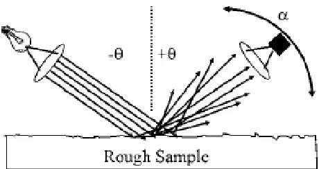
done using a goniophotometer which measures the reflected light as a function of angle

of detection θde, angle of source illumination θso or angle of tilt of the sample α. The

BRDF obtained is a graph of the average irradiance, I, as a function of θde, θso or α

(Arney, et al., 2004). This is illustrated in Figure 5.

If the incident and reflected flux on a surface is considered, the bi-directional reflectance

distributed function is defined as the ratio of directional reflected radiance to the

directional incident radiance. The BRDF is denoted by the symbol f_r and is represented by the equation given below (Nicodemus, Richmond, Hsia, & Ginsberg, 1977).

) , ( / ) ; , ; , ( ) , ; ,

( _{i i r r r i i r r i i i}

r dL E dE

f

θ

φ

θ

φ

θ

φ

θ

φ

θ

φ

Figure 5: A goniophotometer measures the reflected light as a function of (A) the angle of detection θde; (B) the angle of illumination θse; and/or (C) the angle of tilt of the sample, α. Each

10 In the above equation, the subscript i indicates incident radiant flux whereas r indicates reflected radiance flux. Table 1 explains the symbols related to the BRDF (Chen, 2008)

Symbol Term Unit Dimension

Θ Polar Angle [rad]

Φ Azimuth Angle [rad]

E Irradiance [Wm-2]

L Radiance [Wm-2sr-1]

dω Solid Angle [sr]

dA Surface Element [m2]

Figure 6 depicts the BRDF in terms of illumination and viewing angles. In this case, a

surface element (dA) is illuminated from the incident direction (θi, φi) within solid angle

(dωi), with reflection taking place in the direction (θr, φr) within the solid angle (dωr)

11

2.2.2 MEASUREMENT OF SURFACE TOPOGRAPHY

Since the 15th century, artists have applied the laws of geometric perspective to represent

three-dimensional space and shape in two-dimensional images. A number of tools have

been used to characterize shapes and topography. Significant information about the visual

appearance of a surface can be derived from measures of its topographic features.

Photometric stereo is an image-based technique for measuring surface topography that

comes from the field of computer vision.

In the photometric stereo method, the surface orientation is determined from two or more

images by using their corresponding reflectance maps. A reflectance map determines

image intensity as a function of its surface gradients. It represents the surface reflectance

of a material for a particular light source, object surface and viewer geometry.

Reflectance maps are determined empirically, from phenomenological models of surface

reflectivity or derived from analytical models of surface microstructure. The reflectance

map is also related to the bi-directional reflectance distribution function (BRDF) of a

material.

The idea of photometric stereo is to vary the direction of incident illumination between

two successive views, keeping the direction of viewing constant. Since there is no

change in the imaging geometry, each picture element in the images obtained correspond

to the same object point and hence to the same gradient. The varying of the direction of

incident illumination only varies the reflectance map that characterizes the imaging

situation. A combination of these maps can be used to determine the surface orientation

at each image point.

The photometric stereo method is famous because of its simple yet effective

methodology. The only computation required is for the initial determination of the

reflectance map for each experimental situation. Since images are obtained from the same

point of view, it is easy to identify corresponding points in the images. This reduces a lot

12 photometric stereo can be obtained by moving a single light source or my using multiple

light sources calibrated with respect to each other, or by rotating the object surface and

imaging hardware together to stimulate the effect of moving a single light source.

Photometric stereo works best on smooth surfaces with uniform surface properties

(Woodham, 1980).

A simplified application of the photometric stereo method is used by museum

professionals to examine works of art on paper is the raking light method, where the

texture and topography is documented by observing and photographing the object

illuminated with a light source placed at a low angle , measured from the horizontal plane

of the object (Arney & Stewart, 1993).

As illustrated in Figure 7, the topography of a surface is described as a variation in the

height h(x) across the paper, where x is the dimension in the direction of illumination.

This also means that the topography is described as a variation of the tilt angle α(x)

across the surface.

)] ( tan[ /

)] (

[h x dx x

d = α

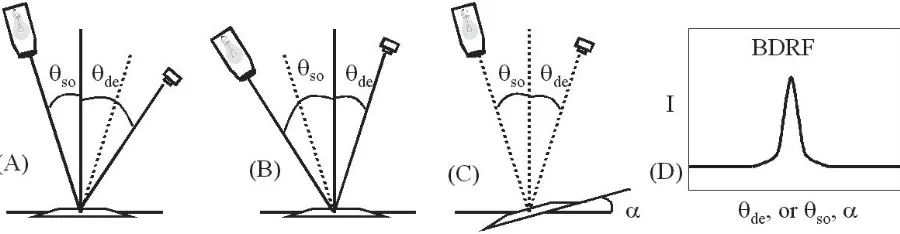
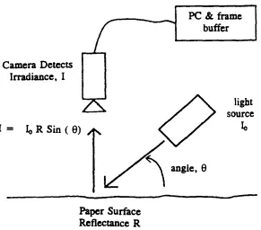
The setup used for image capture using the raking light method is illustrated in Figure 8.

13 The sample is placed in the horizontal plane and is illuminated by a regulated light source

mounted on an arm that can be set at any angle of illumination, θ, between 0° and 90°,

relative to the plane of the sample. A camera is used to detect the irradiance, which is

recorded on a computer. Typically, images are captured of the sample, when it is

illuminated at equal and opposite angles of illumination. One of the assumptions made in

this method is that the sample behaves as a Lambertian reflector, which means that the

material scatters light and appears to have constant brightness, regardless of the angle of

viewing. This implies that the irradiance detected by the camera is not a function of the

angle of viewing of the camera. However, the angle of illumination, θ is directly related

to the apparent brightness of the object as detected at the camera, I, and the reflectance

factor across the surface. Thus, in order to generate the topographical height h(x), the

experimentally observed variations in the pixel values of the two images are examined

and the values of tan[α(x)] are extracted. Pixel by pixel integration of this data can

produce topographical height h(x) (Arney, et al., 1994).

14

2.3 SURFACE MODELING AND RENDERING

Computer graphics image synthesis techniques offer a powerful set of tools for studying

surface appearance. Over the past thirty years computer graphics modeling and rendering

methods have developed from creating crude representations of simple geometric shapes to

being able to produce radiometrically accurate simulations of surfaces with complex

shapes, textures and material properties situated in rich natural lighting environments

(Greenberg, 1997). The basic image synthesis pipeline is illustrated in Figure 9.

The entire process is organized into three parts- the first dealing with the local light

reflection model, the second dealing with the global light transport simulation and finally,

the image display. For the first stage, an accurate physically based light reflection model is

derived for arbitrary reflectance functions. In the next stage, the rendering algorithms

accurately simulate the physical propagation of light energy throughout the modeled

environment. Once accurate results are obtained in the first two stages, the third stage is

reached, which deals with the creation of accurate images perceptually.

2.3.1 LIGHT REFLECTION MODELS

In the modeling stage, a mathematical model of the scene is created by describing the 3D

surface geometry, surface reflectance properties and emissive properties of the light

sources. Material properties are described using light reflection models such as the Phong

15 (Phong, 1975), Ward (Ward, 1992), or Cook-Torrance (Cook & Torrance, 1981) models

that parameterize surface BRDFs. Given a light source, a surface and an observer, a

reflectance model describes the intensity and the spectral composition of the reflected

light reaching the observer. This is determined by the intensity of the light source and the

reflecting ability and surface properties of the material.

2.3.1.1EMPIRICAL MODELS

Empirical or phenomenological models use a combination of functions to capture all the

features of reflection that are commonly observed, such as diffuse reflectance in all

directions and concentration of light scattering in a near specular direction for glossy

materials. Empirical models do not simulate reflection or scattering from basic laws of

physics. They typically consist of mathematical functions that can be controlled by a

small number of parameters.

Lambertian or “ideal diffuse” reflectance is the condition where all light instead of being

reflected in a single direction (specular reflection), is reflected in all directions with the

same radiance. Real materials usually deviate from Lambertian for angles of incidence

greater than 60°, but this model is used for its computational simplicity.

One of the simplest empirical models was proposed by Phong in 1975 (Phong, 1975).

Only two parameters describe the specular component in this model. This model is

popular because of its mathematical simplicity.

The Ward model introduced in 1992 is similar to the Phong model. Ward developed the

imaging gonioreflectometer at the Lawerence Berkeley Laboratory. His model was

derived by fitting the imaging data obtained from this instrument (Ward, 1992). The main

advantages of this model are that it uses only a few simple parameters making it easier to

control, it can be sampled efficiently for Monte Carlo and can model anisotropic surfaces

16 In 1997, Lafortune developed a BRDF model using non-linear parameters for light

reflection functions. His model was able to capture off-specular reflection, increasing

reflectance and retro-reflection (Lafortune, Foo, Torrance, & Greenberg, 1997)

2.3.1.2PHYSICALLY BASED MODELS

Physically based models are also called “first principles” models. They are developed

based on the theory of optics and physics applied to a surface’s microscopic structure.

Thus every parameter in the model represent either the characteristic of the material or its

physical behavior (Chen, 2008).

The first step in developing analytical models is modeling the surface geometry at the

microscopic level. Torrance and Sparrow developed a light reflection model for

roughened surfaces in 1967. This model assumed that the surface area was comprised of

small, randomly dispersed, mirror-like facets. This model also contained a term that

helped to analyze the shadow and masking phenomena. The model helped explain

off-specular peaks that occur when the angle of incidence increases away from the surface

normal (Torrance & Sparrow, 1967).

Blinn further improved the performance of this model and introduced it to computer

graphics (Blinn, 1977). Blinn selected a distribution developed by Trowbridge and Reitz

that modeled the micro-facets randomly oriented and randomly curved. This model was

more accurate than the other models, resulting from better fitting to the measured data.

Cook and Torrance developed a more generic reflection model to describe the directional

distribution of the reflected light and a color shift that occurs as the reflectance changes

with incident angle (Cook & Torrance, 1981). Multiple distribution functions were

included in this model for the distribution of the micro-facets.

The Oren-Nayar model was an extension of the Cook-Torrance model that assumed

17 model was able to predict backscattering, which occurs when facets oriented towards the

light source diffusely reflect some light back to the source. The Blinn and Cook-Torrance

models do not explain backscattering whereas the Oren-Nayar model does not give

off-specular peaks, therefore these models are often used together to produce the full BRDF.

2.3.2 RENDERING

The light reflection model gives the emission, geometry and reflection functions. Once

these are known, in the rendering stage the model serves as input to a light transport

algorithm that simulates how light propagates through the scene. Any point in a scene can

either receive direct light from illumination sources or receive indirect illumination from

surface inter-reflections (Macey, 1997). Tracing every particle of light is nearly

impractical and would require a large amount of computation time. Therefore, four

categories of light transport modeling have emerged, which are described in brief below.

2.3.2.1RASTERIZATION

Rasterization is the task of taking an image described in a vector graphics format (in the

form of shapes) and converting it to a raster image (in the form of pixels or dots) for

output or storage in the form of an image. The most basic algorithm for this method takes

a 3D scene, described in the form of polygons, and renders it onto a 2D surface, usually a

computer monitor (Wiley, Romney, Evans, & Erdahl, 1967). Though rasterization is one

of the fastest rendering techniques, it is largely based on artistic intent and hence is not a

very accurate technique for computer graphics.

2.3.2.2RAY CASTING

In ray casting, once the geometry of the scene is modeled, it is parsed pixel by pixel from

the point of view (eye) outwards, as if casting rays out from the point of view. The idea is

to find the closest object blocking the path of that ray. Using the material properties and

18 Ray casting is used primarily for realtime simulations where detail is not highly

important and can be easily approximated in order to achieve better computational speed

(Macey, 1997). The resulting surfaces have a characteristic “flat” appearance, if no

advanced rendering techniques are used.

2.3.2.3RAY TRACING

In computer graphics, ray tracing is a commonly used method to generate an image by

tracing a path of light through pixels in an image plane and simulating the effect of its

encounters with virtual objects (Nikodym, 2010). Ray casting algorithms cast rays from

the eye into the scene but the rays were traced no further. Ray tracing follows the ray of

light even after it has encountered a surface, which causes a more realistic simulation of

lighting. Effects such as reflections and shadows are a natural outcome of the ray tracing

algorithm when Monte Carlo methods are applied to it. A major disadvantage of ray

tracing however, is computational cost and performance (Macey, 1997).

2.3.2.4RADIOSITY

Radiosity is a method which attempts to simulate the way in which directly illuminated

surfaces act as indirect light sources that illuminate other surfaces. This is also called as

diffuse interaction. It uses the finite element method to solve the rendering equation for

scenes with purely diffuse surfaces. The inclusion of radiosity calculations lends an

element of added realism to the scene because of the way it mimics real world

phenomena. The advantage of radiosity methods is that once the illumination of a scene

is computed, the results are independent of the observer’s position. Therefore, radiosity is

often used as a supplement to ray tracing methods in order to enhance the rendered scene

19

2.3.3 IMAGING

Generating a visual image is the final stage of realistic image synthesis. A major goal of

this stage is to create an image that is perceptually indistinguishable from the actual scene.

At the end of the light transport process, radiometric values at every point of the 3D scene

are known. In the imaging stage, the simulated scene radiances are mapped to produce a

visual image. It has to account for the physical parameters of the display being used, the

perceptual characteristics of the observer and the conditions under which the scene will be

viewed. Most physically based rendering methods described in the section above are able

to accurately simulate the physical behavior of light. But this does not guarantee that the

images developed will have a realistic visual appearance. The first reason for this is the

limitation of display devices in terms of resolution, luminance range and color gamuts.

Secondly, the scene’s observer and display observer may be in different visual states,

affecting their perception of the displayed visual scene.

There are limits on the fidelity of display devices. Tone and gamut mapping are some of

the techniques used to overcome these limitations. Tone mapping is a technique used in

computer graphics to map one set of colors to another, to approximate the appearance of

high dynamic range images in a medium that has a limited dynamic range (like monitors).

Most devices also do not have the same subset of colors which can be accurately

represented on a display device, also called gamut. Gamut mapping is a technique for

transforming the colors of a source image into the color space of the display device that

best reproduces the appearance of the source. These techniques can help achieve a greater

perceptual match between a real scene and displayed scene, even though the display

device is not able to reproduce the full range of luminance and color values.

Improving the visual realism of synthetic images is a still underexplored area of computer

graphics. In order to produce realistic images, one needs to model not only the physical

behavior of light, but also the parameters of perceptual response. This is done by modeling

20 produce an image that accurately represents the visual appearance of the scene from a

21

2.4 PSYCHOPHYSICS

Psychophysics is a branch of psychology that deals with human responses to physical

stimuli, particularly related to the perception of human magnitude. It is described as the

“scientific study of the relation between stimulus and sensation” (Gescheider, 1997).

In the commercial industry, appearance of an object is an importance factor contributing

towards customer satisfaction. Most commonly, the emphasis for the study of appearance

has been on an objective evaluation which involves physical measurement of images. But

at the same time, it is important to also study subjective appearance evaluation, which

focuses on collecting and analyzing judgments from human customers. Customer

perceptions are the visual perceptual attributes that form the basis of the quality preference

of judgment by the customer. The purpose of the psychophysical experiments is to assign

numbers to these attributes. Most psychophysical experiments either involve determination

of thresholds or formulating a psychophysical scale (Engeldrum, 2000).

2.4.1 DETERMINATION OF THRESHOLDS

A threshold is the point of intensity at which a participant can just detect the presence of,

or difference in, a stimulus. Presenting a stimulus to observers and asking them to report

whether or not they perceive it is the basic procedure for measuring thresholds. Some of

the classical methods for stimulus detection or difference detection are described in brief

below (Guilford, 1954).

(i) Method of Limits: This is the most common technique for determining sensory

thresholds. The experimenter initially presents a stimulus well above or well

below the threshold level. On each successive presentation, the threshold is

approached by changing the stimulus intensity by a small amount until the

boundary of sensation is reached. The manipulation can be done in either an

ascending or descending manner.

(ii) Method of Constant Stimuli: In this process, the same set of stimuli is repeatedly

22 trial to the next, but is presented randomly. This prevents the subject from being

able to predict the level of the next stimulus. The 50% threshold is located

somewhere within the range of stimulus values.

(iii) Method of Adjustment: The method of adjustment asks the subject to alter the

level of the stimulus until it is barely detectable against the background noise or is

the same as the level of another stimulus. The difference between the variable

stimuli and the standard one is recorded after each trial.

2.4.2 PSYCHOPHYSICAL SCALING

Although the investigation of sensitivity by measuring absolute and difference thresholds

provides valuable information about the senses, it does not give a complete picture of the

system. Psychophysical scaling methods differ from the traditional methods in that the

end results are not values on physical scales but are on psychophysical scales. Some of

the most commonly used psychological scaling methods are described in brief.

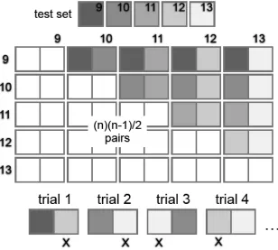
(i) Method of Pair Comparisons: In this method of pair comparisons, all stimuli to be

evaluated on a psychological scale are typically presented to the observer in all

possible pairs. The observer judges whether one of the pair is of greater quantity

than the other in some defined respect. L. L. Thurstone first introduced a scientific

approach to using pairwise comparison for measurement in 1927, which is called

the Thurstone Law of Comparative Judgment. He demonstrated that the approach

could be used to order items along a dimension such as preference or importance,

23 (ii) Method of rank order: This method is popular because of the ease with which

large number of stimuli can be judged with reference to each other. It forces

observers to make the maximum number of discriminations and thus provides as

much information as is possible to obtain from them. Hence this method is similar

to a simultaneous pair comparison method. Any stimuli that can be manipulated

in any manner so that an observer can place them in serial order (from dark to

bright, or rough to smooth), can be analyzed using this method. All the stimuli in

this method are present for simultaneous observation.

(iii) Category Scaling: This method required observers to place stimuli in categories

which may be labeled with names such as “good”, “better and “best” or with

numbers.

(iv) Multidimensional scaling: Multidimensional scaling is a statistical method for

finding the latent dimensions in a dataset. Its most common applications are in

data mining in fields such as cognitive science, psychometrics, etc. Typically,

potential customers are asked to compare pairs of products and make judgments

24 about their similarity or dissimilarity. MDS then obtains the underlying

dimensions from respondents’ judgments about their similarity and reconstructs a

25

2.5 SURFACE APPEARANCE CHARACTERIZATION

As described in Section 1, visual appearance is evaluated using two broad categories of

attributes- those associated with color and those that result from the geometric attributes of a

surface. These geometric attributes can further be classified as gloss and texture, which

describe the spatial distribution of light at the microscale and mesoscale respectively.

2.5.1 COLOR

Color can be considered to be a composite, three-dimensional characteristic consisting of

a lightness attribute and two chromatic attributes called hue and saturation. Color is

related to a surface’s spectral reflectance properties. Many models have been developed

for describing color. The simplest one is the RGB model used in video and computer

graphics. The more sophisticated ones are Munsell, XYZ, CIELAB etc. which have the

psychophysics of color perception as their basis (Hunter & Harold, 1987).

2.5.2 GEOMETRIC ATTRIBUTES

Surfaces can be analyzed at various spatial scaled. Variations at the microscale level

include changes in the microscopic surface structure. This variation causes a difference in

the spatial distribution of light by the object and is called gloss. Gloss depends on a

surface’s directional reflectance properties. It cannot uniquely be described by an

organized coordinate system. If a surface is to be completely described, another important

aspect of its appearance is texture, or the “bumpiness” of the surface. Significant

information about the visual appearance of a surface can be derived from the measures of

its topographical features.

Most models used to describe gloss are based on quantitative studies of light reflection

and though very accurate, the parameters used in these models are unintuitive and do not

26 on the physics of light reflection and at the same time, considers the phenomenology of

gloss perception (Hunter & Harold, 1987).

According to the classic work done by Hunter in 1936, there are around six different

visual phenomena related to apparent gloss (Hunter & Harold, 1987). They are:

(i) Specular Gloss: Perceived surface brightness associated with the specular

reflection from a surface

(ii) Sheen: Perceived shininess at grazing angles seen in otherwise matte specimens

(iii) Distinctness of Image (DOI) Gloss: The sharpness with which images are

perceived after reflection from a surface

(iv) Contrast Gloss (Luster): Perceived relative brightness of brighter and less-bright

areas adjacent to each other on the surface of an object. This takes place because

of selective reflection in directions relatively far from those of specular reflection.

(v) Reflection Haze: Perceived scattering of light (cloudiness) reflected from a

surface in directions near those with specular reflection.

(vi) Absence-of-texture Gloss: Perceived surface smoothness and uniformity.

Judd (Judd, 1937) used Hunter’s observations to formulate expressions that related the

types of gloss to the physical features of surface bi-directional reflectance distribution

functions (BRDFs). Hunter and Judd’s research is important because it was one of the

first to recognize the multi-dimensional nature of gloss perception. Their research has

been used as a framework for all other work related to gloss perception. However, it is

not always easy to correlate their metrics with object appearance under natural conditions

(O'Donnel, 1984).

One of the significant works in the field of gloss perception was done by Billmeyer and

O’Donnell, who tried to address this issue from first principles (O'Donnel & Billmeyer,

1986). They used a set of white, gray and black paints with varying gloss levels and

collected ratings of perceived differences in gloss between pairs of samples. They then

27 Their samples were flat and were viewed under direct illumination with black surround.

From their experiments, they concluded that the appearance of high gloss surfaces is best

described by what Hunter calls distinctness-of-image gloss, and the appearance of low

gloss surfaces is best described by contrast gloss. The only limitation of their work was

that they look at surfaces under uniform surrounds, whereas in order to study perception

of gloss, we need to study objects in realistically rendered environments.

(Ferwerda, 2001) use image synthesis techniques to explore the relationship between

physical dimensions of gloss reflectance and perceptual dimensions of gloss. They used a

set of achromatic glossy paints to conduct two experiments. In their experiments, they

use multidimensional scaling to determine the dimensionality of gloss perception and

create a perceptually uniform “gloss space”. They inferred that gloss has two dimensions,

which are qualitatively similar to the contrast gloss and distinctness-of-image gloss as

described by Hunter. Their work is significant as it attempts to develop a

psychophysically-based light reflection model where the dimensions of the model are

perceptually meaningful and the variations along the dimension are uniform. They also

28

3

EXPERIMENTS

The touch-up effect is essentially a visual problem. Touch-up visibility can broadly depend on

surface properties or environmental conditions. Surface properties are governed at the microscale

by the reflectance of the surface and at the mesoscale, by the surface texture. In practical terms,

these are interlinked with the paint formulation and application methods. Environmental

conditions include the lighting and viewing conditions prevalent in the surroundings. Modifying

these environmental factors can increase or decrease the perceptual magnitude of the touch-up

problem.

In order to develop an understanding of the factors that have the greatest influence, it was

necessary to first perform a qualitative analysis of the touch-up problem. This was done using

two psychophysical experiments aimed towards determining the effect of the various surface and

environmental conditions on the visibility of the touch-up region.

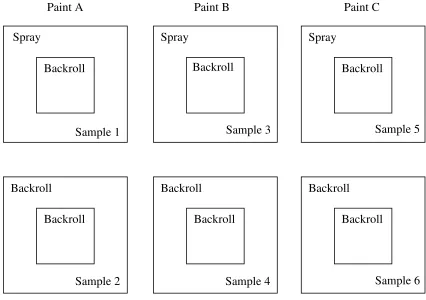
3.1 SAMPLE PREPARATION

The first step to performing the psychophysical experiments was creation of touch-up

samples. Six different samples were created by applying flat interior latex house paint to a

2’ by 2’ panel of standard paper coated gypsum wallboard. Three types of paints (A, B, C)

were used, each of them varying in their chemical formulations. Two commonly used

application methods were used- airless spraying and rolling.

Initially, a base coat was applied over the whole panel- three panels each using spraying and

rolling methods. Once this coat had dried, a 1’ by 1’ region in the center of the panel was

“touched-up” with a second coat applied with a fabric roller. Each of the panels was

29

Paint A Paint B Paint C

3.1.1 LIGHT SOURCE SELECTION

Physical inspection of the samples under different lighting and viewing conditions

illustrated the touch-up effect. However, in order to obtain measurable results, it was

important to be able to document this effect. The easiest way to do this was to attempt to

recreate these real-time observations using physical photographs. Various lighting and

viewing configurations were used in order to finalize the arrangement that best captures

this effect.

In order to explore the effects of light source geometry on the touch-up visibility, the

samples were first photographed with a point, linear and area light source. A 5’ by 7’

Spray Spray Spray

Backroll Backroll Backroll

Backroll Backroll Backroll

Backroll

Backroll Backroll

Sample 1 Sample 3 Sample 5

Sample 2 Sample 4 Sample 6

30 white LED light box was used and sections of the light box were masked off using

cardboard to simulate the different lighting geometries. Samples were photographed with

the light source and camera at 60° from the normal.

From these images, it was evident that the area light source was more effective in

capturing the differences between the base and touch-up regions, compared to a point or

linear light source. In the first two images, there is a very specific “hot-spot” causing

uneven illumination across the image. This problem is eliminated with the use of an area

light source. Also, the area light source can also be used to simulate lighting from a

window or overhead fixture, as would be the case in most natural environments. Hence, it

was decided to use an area light source.

31

3.1.2 SELECTION OF CONFIGURATIONS

To verify that the sample produced a measurable touch-up effect, we photographed it

with a Canon EOS XSi 12 Megapixel digital camera. The camera was set to provide good

depth of field and good noise response. A 28-105 mm lens was used with the lens

completely zoomed in (105 mm). The ISO was set to 100 and aperture was set to F29.

The field of view obtained at this setting was 20°. The camera and light source were

placed at a distance of 60 cm from the sample. The images were captured in the Canon

RAW (CR2) format with an Adobe RGB colorspace.

The samples were photographed at a range of illumination angles from 40° to 80° off the

surface normal. The camera was first placed at an angle of 0° (normal to the samples),

and then at 60° off the surface normal and opposite to the light source. An analysis of

these images helped get an idea of how the touch-up effect manifests itself at different

configurations. The purpose of this experiment was to identify the configurations that

would represent the best and worst cases of touch-up visibility. Figure 13 shows the

series of images produced by focusing on the edge between the sprayed base region (left

half of each image) and the rolled touch-up region (right half of each image). The

viewing is oblique, at 60° off the surface normal. Each panel shows the appearance at a

particular illumination angle. As is observed, there is a visible difference in surface

texture and lightness as illumination goes from near normal (40°) through specular (60°)

to grazing (80°). The distinct difference in surface lightness and texture can be seen

between the two regions, with the base region generally appearing smoother and lighter

32 65°

67.5°

70°

72.5°

75°

80° 40°

45°

50°

55°

60°

62.5°

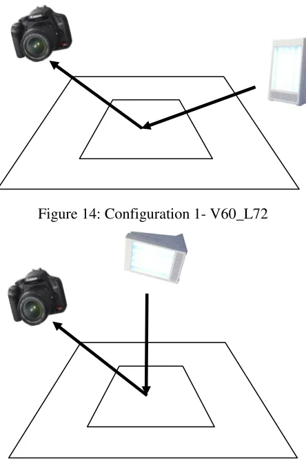
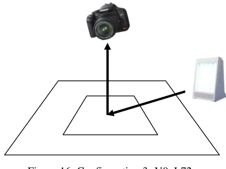
33 Observation of the image set showed that the touch-up visibility is most pronounced

when the sample is illuminated at 72°. This was identified as the potential “worst-case”

scenario. Comparing this with normal viewing and specular lighting revealed that in this

configuration, shadowing was an important factor that contributed to appearance

differences. To lend symmetry to the experiment, images were also taken at normal

lighting and grazing viewing, where lightness differences were more enhanced.

Configuration Camera Angle Illumination Angle

1 60° 72°

2 60° 0°

3 0° 72°

Figure 14: Configuration 1- V60_L72

Figure 15: Configuration 2- V60_L0

34

3.2 DESIGN OF PSYCHOPHYSICAL EXPERIMENTS

The aim of the psychophysical experiments was to determine the smallest perceptible

difference (or just noticeable difference) in touch-up visibility. Hence, it was decided to use

a Two-Alternative Forced Choice (2AFC) procedure for the experiments. In this design,

pairs of stimuli are shown to the subject and they are forced to make a choice between them,

even if they cannot detect a difference. Two experiments were designed, each with specific

objectives in mind. The purpose and experimental design is described below.

3.2.1 EXPERIMENT 1

The purpose of the first experiment was to determine the effects of four variables- paint

formulation, application methods and lighting and viewing conditions on touch-up

visibility. Hence, the main experimental design consisted of images that captured a wide

range of touch-up differences. The following conditions were used:

(i) Types of Paints- A, B, C

(ii) Types of Application Methods- Spray and Roll

(iii) Types of Viewing/Lighting combinations- V60_L72, V0_L72, V60_L0

Hence, the total number of stimulus images = 3 paints x 2 application methods x 3

configurations = 18 images

Number of trials = 18 x (18-1)/2 = 153 trials

35

3.2.2 EXPERIMENT 2

Experiment 1 will help establish the visibility of the touch-up region as a function of the

paint formulation, application method, lighting and viewing condition. The purpose of the

second psychophysical experiment is to study whether the edge has an effect on the

human perception of a difference in appearance between the two regions. There was a

possibility that the distinct edge present between the base and touch-up replicated a

Craik-O’Brien-Cornsweet illusion when viewed by an observer.

The Craik-O’Brien-Cornsweet effect is a visual illusion where luminance of enclosed

boundaries sets the brightness of the enclosed regions (Cornsweet, 1970). For example,

consider Figure 17 below. The region to the right of the edge appears slightly lighter than

the region to the left of the edge. But if the central region is blackened out, thus

“removing” the edge, it can be seen that the two areas in fact have the exact same

brightness. Figure 18 shows the difference between the actual distributions of luminance

in the image versus the perceived distribution.

36 For this experiment, it was necessary to physically create different “types of edges”, in

order to judge the effect of the contours on the touch-up visibility. Only the images from

the worst case scenario (V60_L72) were used in this experiment. In order to estimate the

placement of the edge samples above or below the threshold based on the natural

variance in the spray and rolled sides, the images of only the base regions of paint C were also included in the study. These were called “Null” images. The reason for including

only paint C is that it has the least visible differences between the base and touch-up

regions. Hence, the following conditions were used:

(i) Types of Paints: A, B, C

(ii) Types of Application Methods: Spray and Roll

(iii) Types of Lighting/Viewing Combinations: V60_L72

(iv) Types of Edges (described in detail on Page 40): Normal, Sharp, Blend + 2 Nulls

Hence, number of stimulus images = 3 paints x 2 application methods x 1

lighting/viewing condition x 3 edges + 2 nulls = 20 images

Number of trials = 20 x (20-1)/2 = 190 trials

37

3.3 STIMULUS PREPARATION

As mentioned earlier, the images captured using the digital camera was in the Canon RAW

(CR2) format. They needed to be processed to make the stimuli suitable for each of the

experiments. The detailed procedure used for processing the stimuli for each experiment is

described below.

3.3.1 EXPERIMENT 1

The CR2 images that were captured using the camera could not be used as-is for the

experiments. The field of view was 20° with the focus set to the edge between the base

and touch-up. Hence region outside the FOV needed to be cropped out. Secondly, since

the sample was illuminated at an angle, the luminance across the horizontal plane of the

image was not equally distributed. These modifications needed to be made in order to

process the images for the experiments. The following steps were performed:

(i) Central 1200x600 pixel sections were cropped from the original 4272x2848 pixel

images such that the edge is approximately centered in the image.

(ii) The embedded color profile was discarded and the G-channel was converted to

grayscale

(iii) A high-pass filter was applied to equalize luminance across the image

These images were termed the “normal” set of images for the six samples.

38

3.3.2 EXPERIMENT 2

The initial processing was the same as described to create the “normal” image set for

Experiment 1. Following this, the following types of edges were created using

Photoshop.

(i) Normal edge: The original edges on the samples were used as-is, without any

modifications

(ii) Sharp edge: Sections of the base and touch-up regions excluding the edge were

cropped and placed side by side to create a sharp, straight-line edge.

Figure 20: Stimulus preparation for Experiment 2. The image to the right represents the normal edge stimulus for Sample 1 at V60_L72 configuration

39 (iii) Blend edge: The transparency of the edge in the sharp images was modified so

that it appears to blend in with the surrounding base and touch-up

(iv) Null sample: A 1200x600 crop-out of just the base region for sample with paint C

was used to create the null images.

3.4 EXPERIMENTAL PROCEDURE

30 subjects, ages 20 to 40, participated in each experiment. They were all naïve to the

methods of the experiment. All had normal or corrected to normal vision.

Figure 22: Stimulus preparation for Experiment 2. The image to the right represents the blend edge stimulus for Sample 1 at V60_L72 configuration

40 In the experimental session, the subjects viewed pairs of images displayed on a calibrated

30-inch Apple Cinema display. The monitor resolution was set to 2560x1600 and the

system gamma was 2.2.