Multitrace formulations and Dirichlet-Neumann algorithms

Multitrace formulations and

Dirichlet-Neumann algorithms

Victorita Dolean1 _{and Martin J. Gander}2

1 Introduction

Multitrace formulations (MTF) for boundary integral equations (BIE) were developed over the last few years in [4] and [1, 2] for the simulation of elec-tromagnetic problems in piecewise constant media, see also [3] for associated boundary integral methods. The MTFs are naturally adapted to the devel-opments of new block preconditioners, as indicated in [5], but very little is known so far about such associated iterative solvers. The goal of our presen-tation is to give an elementary introduction to MTFs, and also to establish a natural connection with the more classical Dirichlet-Neumann algorithms that are well understood in the domain decomposition literature, see for ex-ample [6, 7]. We present for a model problem a convergence analysis for a naturally arising block iterative method associated with the MTF, and also first numerical results to illustrate what performance one can expect from such an iterative solver.

2 One-dimensional example

In this section we introduce the Calderon projectors and the multitrace for-mulation for the one dimensional model problem

Au:=u′′(x)−a2u(x) = 0, a >0. (1)

The family of bounded solutions of (1) on the domains Ω± = R± _{is given} by u(x) =Ce∓ax, where C =u(0). We say that the solution spaces of the operatorA onR± _{are given by}

Z±={u∈L2(Ω)|u(x) =Ce∓ax, C∈R}=Re∓ax.

Note that anyu±∈Z± _{satisfies the relationu}′

±(0) =±au±(0) and thus the space of all possible Cauchy data of the solutions of (1) onR± _{is given by}

V±={(g0, g1) =C(1,±a), C∈R}=R

1

±a

.

University of Strathclyde and University of Nice-Sophia [email protected]·

Uni-versity of Geneva, [email protected]

Definition 1 (Calderon projectors). Letρ±_:Z±_→V± _{be the operator} that associates to any solution ofAu= 0 onR±_{its pair of traces (u(0), u}′_(0)). LetK± :R2_→Z± _{be the operator that associates to any pair (h}

0, h1)∈R2

the quantity K±(h0, h1) = c∓e∓ax, where u(x) = c+eax +c−e−ax is the

unique solution of (1) with Cauchy data (g0, g1),

Au= 0, u(0) =h0 andu′(0) =h1. (2)

Calderon projectorsare defined as the projections P±:R2_→V±_{, such that}

P±=ρ±◦K±. (3)

The expressions of P± _{for our model problem can be computed explicitly.} The solution of (2) is

u(x) = 1

2a(ah0+h1)e ax₊ 1

2a(ah0−h1)e −ax_,

and thusK±(h0, h1) = ₂1_a(ah0∓h1)e∓ax and

P±(h0, h1) := (ρ±◦K±)(h0, h1) = ₁

2a(ah0∓h1)

∓1

2(ah0∓h1)

⇒P± =

₁ 2 ∓

1 2a

∓a

2 1 2

.

Remark 1.From the previous construction we see that the Calderon projector

is unique. When working with subdomains, it is however more convenient to introduce normal derivatives at interfaces, instead ofu′(0), and we thus define the Calderon projectors for normal derivatives with the modified sign

P±(h0, h1) :=P±(h0,∓h1)⇒P+=P−= ₁

2 1 2a a

2 1 2

, (4)

and we will useP± _{in what follows.}

Definition 2 (Multitraces). Following the notations in [4], we denote by

T±u:=

u(0)

∓u′₍₀₎

(5)

the multitrace (Dirichlet and Neumann) on the boundary {x= 0}of a solu-tionuof the equationAu= 0 posed on the half spaceR±_.

Suppose now we have a decomposition ofR into two subdomains Ω1 =Ω−

and Ω2 =Ω+ and we want to solve equation (1) by an iterative algorithm

involving Dirichlet and Neumann traces on the interface {x = 0}. LetT1,2

be the trace operators as defined in (5) (T1 = T− _{and T2 = T}+_{) for the}

subdomainsΩ1,2, andP1,2 the corresponding Calderon projectors as defined

Definition 3 (Multitrace formulation).Themultitrace formulationfrom [4] states that the pairs (Tiui)i=1,2 are traces of the solution defined onΩi if they verify the relations

      

(P1−I)T1u1−σ1

T1u1−

1 0 0−1

T2u2

= 0,

(P2−I)T2u2−σ2

T2u2−

1 0 0−1

T1u1

= 0,

(6)

whereσ1,2 are some relaxation parameters.

We see that a natural iterative method (also introduced in [5]) for (6) starts with some initial guesses (u0

i, vi0)i=1,2 for the traces, and computes for n=

1,2, . . .the new trace pairs from the relations

      

(P1−I)

un1

vn1

−σ1

un1

vn1

=−σ1

un−2 1 −vn−₂ 1

,

(P2−I)

un2

vn2

−σ2

un2

vn2

=−σ2

un−1 1 −vn−₁ 1

.

(7)

By introducing the expressions ofPi, we can rewrite the iteration in the form

   

−(σ1+1₂) ₂1_a

a

2 −(σ1+ 1 2)

−(σ2+1₂) ₂1_a 1

2 −(σ2+ 1 2)         un 1 vn 1 un 2 vn 2    =    

−σ1un−2 1

σ1v2n−1 −σ2un−1 1

σ2v1n−1    ,

(8) or when solving for the new iterates

    un 1 vn 1 un 2 vn 2    =

0 A1

A2 0

   

un−₁ 1 v₁n−1 un−₂ 1 v₂n−1

   =:A

   

un−₁ 1 vn−₁ 1 un−₂ 1 vn−₂ 1

  

, (9)

where

Ai= 1

2(σi+ 1)

2σi+ 1 −1

a a −(1 + 2σi)

, i= 1,2.

The convergence factor of (7) is therefore given by the spectral radius of the iteration matrixA, whose eigenvalues are

λ(A) :=

−

r

σ1

σ1+ 1

,

r

σ1

σ1+ 1

,− r

σ2

σ2+ 1

,

r

σ2

σ2+ 1

. (10)

We see that the convergence factor is independent ofaand thus only depends on the relaxation parametersσi. If we suppose by symmetry thatσ1=σ2=:

σ, the convergence factor becomes ρ(A) = q σ

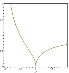
Fig. 1 Convergence factor of the iterative multitrace formulation in 1d as function of the relaxation parameterσ

ρ(A) as a function ofσ in Figure 1. We see that the algorithm diverges for σ < −1

2, stagnates forσ = − 1

2 and converges for σ > − 1

2. For σ = 0, the

convergence factor vanishes, but a closer look at the iteration formula (8) shows that the matrix is then singular and thus the algorithm is no longer well defined for this value. On the other hand, the associated iteration (9) is still well defined, the latter being equivalent to (8) only for σ6= 0. Overall, we see that algorithm (8) converges rapidly when the relaxation parameter is chosen close to 0.

3 Two-dimensional example

Suppose we want to solve the Laplace equation

uxx+uyy = 0, in Ω=R2_{, (11)}

using the two subdomainsΩ1:=R−×RandΩ2:=R+×Rand a multitrace

formulation. To use our results from the previous section we take a Fourier transform in they variable,

ˆ

uxx−k2uˆ= 0. (12)

We can now follow the reasoning of the previous section in Fourier space, replacingaby|k|. Thus any given pair of boundary functions (ˆh0(k),ˆh1(k))

can be projected to become compatible boundary traces using the symbol of the the Calderon projectors

b Pi

_ˆ

h0

ˆ h1

=

" ₁ 2

1 2|k| |k|

2 1 2

# _ˆ

h0

ˆ h1

We next express the Calderon projectors in terms of Dirichlet-to-Neumann (DtN) and Neumann-to-Dirichlet (NtD) operators.

Lemma 1 (Calderon projectors and DtN operators).Calderon

projec-tors can be written in terms of the local DtN and NtD operaprojec-tors as

b Pi=

1 2

"

1 \N tDi

\

DtNi 1

#

, i= 1,2, (14)

where DtNi associates to given Dirichlet data ˆg0 on the interface x = 0

the normal derivative ∂ui

∂ni of the solution ui in Ωi and the N tDi associates

to given Neumann data gˆ1 on the interface x = 0 the trace of the solution

ˆ

ui(0, k)on the same boundary.

Proof. OnΩ1, we obtain explicitly the symbols of these operators from

ˆ

u1(x, k) = ˆg0e|k|x⇒

∂uˆ1

∂x|x=0=|k|ˆg0⇒DtN\1=|k|, ˆ

u1(x, k) = ˆu1(0, k)e|k|x,

∂uˆ1

∂x |x=0= ˆg1⇒uˆ1(0, k)|k|= ˆg1⇒N tD\1= 1

|k|.

The corresponding symbols for the domainΩ2 are

\

DtN2=|k|, N tD\2=

1

|k|.

Inserting these expressions into (14) concludes the proof.

We are ready now to establish the link between these algorithms and the classical DtN iterations.

Theorem 1 (Link with the DtN iterations). The iterative multitrace

formulation for the special choice σ1 = σ2 = −1₂ computes simultaneously

a Dirichlet-Neumann iteration (un

1, vn2) and a Neumann-Dirichlet iteration

(vn

1, un2)without a relaxation parameter.

Proof. According to the results of Lemma 1, in two dimensions, iteration (7)

becomes

1 2

"

−1−2σ1 N tD\1 \

DtN1 −1−2σ1 #

ˆ un1

ˆ v1n

=−σ1

ˆ un−2 1 −ˆvn−₂ 1

,

1 2

"

−1−2σ2 N tD\2 \

DtN2 −1−2σ2 #

ˆ un

2

ˆ vn

2

=−σ2

ˆ un−₁ 1

−ˆvn−₁ 1

.

(15)

We see that for the special choiceσ1=σ2=−1₂, iteration (15) simplifies to (

\

N tD1vˆ1n= ˆu

n−1 2 , \

DtN1uˆn1 =−vˆ

n−1 2 ,

( \

N tD2ˆvn2 = ˆu

n−1 1 , \

DtN2uˆn2 =−ˆv

n−1 1 .

From the symbols, we see that N tDi\−1 = \DtNi, and hence iteration (16)

becomes ₍

ˆ vn

1 =DtN\1uˆn−2 1,

ˆ un

1 =−N tD\1vˆ2n−1, (

ˆ vn

2 =DtN\2uˆn−1 1,

ˆ un

2 =−N tD\2ˆv1n−1,

(17)

which leads to the conclusion.

In order to study the role of the relaxation parameters σi, we check first under which conditions iteration (15), written explicitly as

B1

ˆ un

1

ˆ v1n

:=1 2

−1−2σ1 _|k|1 |k| −1−2σ1

ˆ un

1

ˆ vn1

=−σ1

ˆ un−₂ 1

−vˆn−₂ 1

,

B2

ˆ un

2

ˆ vn

2

:=1₂

₋₁₋₂

σ2 _|k|1 |k| −1−2σ2

ˆ un

2

ˆ vn

2

=−σ2

ˆ un−₁ 1

−vˆn−1 1

,

(18)

is well defined. This is the case if the matrices Bi are invertible. Since det(Bi) = 4σi(σi+ 1),the multitrace iteration is well defined ifσi 6={0,−1}. In this case (18) is equivalent to

ˆ un

1

ˆ vn

1

=B1−1

ˆ un−₂ 1 ˆ v₂n−1

=

1+2σ1

2(σ1+1)uˆ

n−1

2 −2(σ11+1)N tD\1ˆv

n−1 2 1

2(σ1+1)DtN\1uˆ

n−1

2 −2(1+2σ1+1)σ1 vˆ

n−1 2

!

,

ˆ un

2

ˆ vn

2

=B₂−1

ˆ un−₁ 1 ˆ v₁n−1

=

1+2σ1

2(σ1+1)uˆ

n−1

1 −2(σ11+1)N tD\2ˆv

n−1 1 1

2(σ1+1)DtN\2uˆ

n−1

1 −2(1+2σ1+1)σ1 vˆ

n−1 1

!

.

(19)

Algorithm (19) has the same convergence properties as (9), since we obtain the same convergence factor independent of the Fourier variable k, which means convergence is going to be mesh independent.

4 Numerical results

We now show some numerical experiments for illustration purposes on our two-dimensional model problem (11) on the domain Ω = (−1,1)×(0,1) decomposed into the two subdomainsΩ1= (−1,0)×(0,1) andΩ2= (0,1)×

−1 −0.5 0 0 0.5 1 −1 0 1 x y u1 −1 − 0.5 0 0 0.5 1 −1 0 1 x y v1 0 0.5 1 0 0.5 1 −1 0 1 x y u2 0 0.5 1 0 0.5 1 −1 0 1 x y v2 −1 −0.5 0 0 0.5 1 −1 0 1 x y u1 −1 −0.5 0 0 0.5 1 −1 0 1 x y v1 0 0.5 1 0 0.5 1 −1 0 1 x y u2 0 0.5 1 0 0.5 1 −1 0 1 x y v2

Fig. 2 Evolution of the error forσ=₋0.6 after 2 Iterations (left), 10 iterations (right)

−1 −0.5 0 0 0.5 1 −1 0 1 x y u1 −1 − 0.5 0 0 0.5 1 −1 0 1 x y v1 0 0.5 1 0 0.5 1 −1 0 1 x y u2 0 0.5 1 0 0.5 1 −1 0 1 x y v2 −1 −0.5 0 0 0.5 1 −1 0 1 x y u1 −1 −0.5 0 0 0.5 1 −1 0 1 x y v1 0 0.5 1 0 0.5 1 −1 0 1 x y u2 0 0.5 1 0 0.5 1 −1 0 1 x y v2

Fig. 3 Evolution of the error forσ=₋0.5 after 2 Iterations (left), 10 iterations (right)

−1 − 0.5 0 0 0.5 1 −1 0 1 x y u1

−1 −

0.5 0 0 0.5 1 −1 0 1 x y v1 0 0.5 1 0 0.5 1 −1 0 1 x y u2 0 0.5 1 0 0.5 1 −1 0 1 x y v2 −1 − 0.5 0 0 0.5 1 −1 0 1 x y u1

−1 −

0.5 0 0 0.5 1 −1 0 1 x y v1 0 0.5 1 0 0.5 1 −1 0 1 x y u2 0 0.5 1 0 0.5 1 −1 0 1 x y v2

Fig. 4 Evolution of the error forσ= 0.1 after 2 Iterations (left), 10 iterations (right)

5 Conclusion

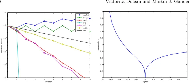
0 1 2 3 4 5 6 7 8 9

10−4

10−3

10−2

10−1

100

101

iteration

maximum error u1

m=−0.6

m=−0.5

m=−0.1 m=0 m=0.1 m=0.5 m=1

−1 −0.8 −0.6 −0.4 −0.2 0 0.2 0.4 0.6 0.8 1

0 0.2 0.4 0.6 0.8 1 1.2 1.4 1.6 1.8 2

sigma

numerical rho

Fig. 5 Error in the maximum norm as a function of the iteration number for different

values ofσ(left), and numerically measured contraction factor of the multitrace iteration

as function ofσ(right)

choices for the relaxation parameter in the multitrace iteration, which was confirmed by numerical experiments.

References

[1] Xavier Claeys and Ralf Hiptmair. Electromagnetic scattering at compos-ite objects: a novel multi-trace boundary integral formulation. ESAIM

Math. Model. Numer. Anal., 46(6):1421–1445, 2012.

[2] Xavier Claeys and Ralf Hiptmair. Multi-trace boundary integral formu-lation for acoustic scattering by composite structures. Comm. Pure Appl.

Math., 66(8):1163–1201, 2013.

[3] Xavier Claeys, Ralf Hiptmair, and Elke Spindler. A second-kind Galerkin boundary element method for scattering at composite objects. Technical Report 2013-13 (revised), Seminar for Applied Mathematics, ETH Z¨urich, 2013.

[4] R. Hiptmair and C. Jerez-Hanckes. Multiple traces boundary integral formulation for Helmholtz transmission problems. Adv. Comput. Math., 37(1):39–91, 2012.

[5] R. Hiptmair, C. Jerez-Hanckes, J. Lee, and Z. Peng. Domain decompo-sition for boundary integral equations via local multi-trace formulations. Technical Report 2013-08 (revised), Seminar for Applied Mathematics, ETH Z¨urich, 2013.

[6] Alfio Quarteroni and Alberto Valli. Domain Decomposition Methods for

Partial Differential Equations. Oxford Science Publications, 1999.

[7] Andrea Toselli and Olof Widlund. Domain Decomposition Methods

-Algorithms and Theory, volume 34 ofSpringer Series in Computational