A Composite Ultrasonic Transducer with a Fractal Architecture

Fractal Architecture

Ebrahem A. Algehyne and Anthony J. Mulholland

Department of Mathematics and Statistics

University of Strathclyde

Livingstone Tower, 26 Richmond Street

Glasgow, UK

G1 1XH

derive a mathematical model to predict the dynamics of an ultrasound transducer that achieves this range of length scales by adopting a frac-tal architecture. In fact, the device is modelled as a graph where the nodes represent segments of the piezoelectric and polymer materials. The electrical and mechanical fields that are contained within this graph are then expressed in terms of a finite element basis. The structure of the resulting discretised equations yields to a renormalisation methodology which is used to derive expressions for the non-dimensionalised electrical impedance and the transmission and reception sensitivities. A compari-son with a homogenised (standard) design shows some benefits of these fractal designs.

1

Introduction

Ultrasonic transducers are devices that are used to convert energy from one

form to another [6]. In this context, they convert energy from its electrical form

improve the transmission and reception sensitivities [13, 29], composite

struc-tures are utilized in piezoelectric ultrasonic transducers. Many biological species

such as dolphins, bats, etc, naturally produce and receive ultrasound by utilising

a wide variety of intricate geometries in their transduction ’equipment’; often

with resonators spread over a range of length scales [26, 25, 20, 7, 9, 27, 31, 8].

However, the man-made transducers tend to employ a regular geometry on a

single length scale. Due to this characteristic, the man-made transducers are

unable to operate over a wider range of frequencies resulting in transmission

and reception sensitivities with narrow bandwidths. To produce transducers

with wider bandwidths, structures with a range of geometrical components need

to be mathematically modelled. One such structures is a fractal [23, 24, 28]. One

approach to designing a new transducer is to experimentally assess its operating

ability, however this is very time consuming. Each device requires materials to

be sought, cut to the desired shape, bonded to other components such as

inatch-ing and backinatch-ing layers, and is expensive and time consuminatch-ing. In addition, to

determine its transmission sensitivity the device has to be immersed in a

wa-ter tank, input voltages of different frequencies are applied, and a hydrophone

placed at some distance from the transducer monitors the output. An

assess-ment can also be made by connecting the transducer to an electrical circuit and

measuring its electrical impedance over a range of frequencies. Given the large

ual edges which, when joined to other edges from the lattice, led to the global

dynamics of the device. To account for the three dimensional world that the

de-vice is embedded within, this paper will derive the governing equations from the

general tensor equations. This framework enables the deployment of different

parameterisations and a scenario where the displacement acts out of the plane of

the lattice with the electric field operating within the plane of the lattice will be

examined in this paper. We will use a finite element methodology and introduce

new basis functions to express the wave fields within the lattice. This Galerkin

approach leads to discrete formulation that lends itself to a renormalisation

ap-proach. The Sierpinski gasket will be used for the simulation of a self-similar

transducer in this paper [10, 32]. Such an ultrasonic transducer would start

with an equilateral triangle of piezoelectric crystal. This equilateral triangle is

composed of four identical equilateral sub-triangles whose side length is half of

the original. The first generation (n = 1) would be obtained by replacing the central sub-triangle by a polymer material. This process is then repeated for

several generations with the removed sub-triangles from the smallest triangles

polymer triangle has a vertex denoted by a non-filled circle which was degree

3 whereas each piezoelectric triangle has a vertex denoted by a filled circle and

has degree 4. The lattice has side lengthL units which remains constant as the generation level n increases. Therefore, as n increases, the length of the edge between adjacent vertices tends to zero and in this limit the lattice will perfectly

match the space filling properties of the original Sierpinski gasket [21]. The total

number of vertices is N∗ _{= 3}n_{+ 3}n−1 _=N(n)_{+ 1 where N}(1) _{= 3 andN}(2) _{= 11}

(see Figures 3 and 4) and h(n) _{= L/(2}n_{− 1) is the edge length between any}

two adjacent piezoelectric vertices. The piezoelectric vertex degree is 4 (apart

from the boundary vertices (input/output vertices) which have degree 3) and

M = (5_×3n_{−3)/2 denotes the total number of edges. These boundary vertices}

will be used to interact with external loads (both electrical and mechanical) and

so we introduce fictitious vertices A, B and C to accommodate these interfacial boundary conditions (see Figures 3 and 4). Denote by Ω the set of points lying

on the edges or vertices of SG(3,4) and denote the region’s boundary by ∂Ω. Note that the edges joining the piezoelectric nodes to the polymer nodes are

composed of a piezoelectric section (shown by the full line in Figure 3 along the

edge joining node 1 to 4) and a polymer section (shown by the dashed line along

this same edge). In what follows we will retain the freedom to vary the fraction

of piezoelectric material in this edge from ν = 1 (piezoelectric material only) to

n= 1 n= 2 n = 3

Figure 2: The first few generations of the Sierpinski gasket lattice SG(3,4).

2

Model Derivation

The lattice represents the vibrations of piezoelectric and polymer materials (here

the focus will be on PZT-5H and HY1300/CY1301 hardset [30] respectively) that

have been manufactured to form a Sierpinski gasket. The interplay between the

electrical and mechanical behaviour of the lattice vertices is described by the

piezoelectric constitutive equations [37, 36]

mation convention is adopted). The strain tensor is related to the displacement

gradients ui,j by

Sij = ui,j +uj,i

2 , (3)

and the electric field vector is related to the electric potential φ via

Ei =₋φ,i. (4)

The dynamics of the piezoelectric material is then governed by

ρEui¨ =Tji,j, (5)

subject to Gauss’ law

Di,i = 0 (6)

whereρE _{is the density andui is the component of displacement in the direction}

of the ith _{basis vector. So, combining equations (5) and (1) gives}

ρE_u¨

i =cjiklSkl,j−ekjiEk,j. (7)

Combining equations (6) and (2) gives

Di,i =eiklSkl,i+εikEk,i= 0. (8)

We will restrict attention to the out of plane displacement only (a horizontal

shear wave) by stipulating that

u= 0,0, u3(x1, x2, t)

Sij =       

1

2u3,2 i= 2, j = 3 ori= 3, j = 2

0 otherwise,

(11)

so equation (10) gives

ρEu¨3 =c1331u3,11+c1332u3,21+c2331u3,12+c2332u3,22−ekj3Ek,j. (12)

From the properties of PZT-5H (see Appendix 11.2), then

ρEu¨3 =c44(u3,11+u3,22)−ekj3Ek,j. (13)

since c55 =c44 and the Voigt notation has been used to express these tensors as

matrices. For example,c44≡c2323ande24≡e223. Now ifE = E1(x1, x2), E2(x1, x2),0

then

ρEu¨3 =c44(u3,11+u3,22)−e113E1,1−e123E1,2−e213E2,1 −e223E2,2. (14)

That is

ρEu¨3 =c44(u3,11+u3,22)−e15E1,1−e14E1,2−e25E2,1−e24E2,2. (15)

That is, for PZT-5H,

e15u3,11+e24u3,22+ε11E1,1+ε22E2,2 = 0. (18)

Therefore

e24(u3,11+u3,22) +ε11(E1,1+E2,2) = 0 (19)

since ε11 =ε22 for PZT-5H. So we get

E1,1+E2,2 =−

e24

ε11

(u3,11+u3,22). (20)

Substituting this equation into equation (16) gives

ρEu¨3 =c44(u3,11+u3,22) +

e2 24

ε11

(u3,11+u3,22). (21)

A similar analysis can be conducted for the polymer phase. The dynamical

equation in each phase can be written as

¨

u3 =c2∇2u3 (22)

where cis the shear wave velocity defined as

c= 

 

 

cT =

p

cT

44/ρE, cT44=c44E +e224/εE11, PZT-5H

cP =

p

cP

44/ρP, polymer

(23)

and _∇2 _{= ∂}2_/∂x2

1 +∂2/∂x22. cT44 is the piezoelectrically stiffened shear

modu-lus in the ceramic phase, cP

q2 u¯= h

2

c2

T

c2 _∇2u.¯ (25) We will seek a weak solution ¯u _∈ H1_{(Ω) where on the boundary ¯u = ¯u}

∂Ω ∈

H1_{(∂Ω). Now multiplying by a test functionw∈H}1

B(Ω), whereHB1(Ω) :={w∈ H1_{(Ω) : w = 0 on∂Ω}, integrating over the region Ω, and using Green’s first}

identity R

Ωψ ∇

2_{φ dv =}H

∂Ωψ(∇φ.n)dr−

R

Ω∇φ.∇ψ dv, where n is the outward

pointing unit normal of surface element dr, gives Z

Ω

q2 u w dx¯ = h

2 c2 T c2 I ∂Ω

w(_∇u.n¯ )dr₋ h

2 c2 T c2 Z Ω∇ ¯

u._∇w dx. (26) Now h2H

∂Ωw(∇u.n¯ )dr is zero since w = 0 on ∂Ω and so, we seek ¯u ∈ H 1_(Ω) such that q2 Z Ω ¯

u w dx=₋h

2 c2 T c2 Z Ω∇ ¯

u._∇w dx (27) where w_∈H1

B(Ω).

3

Galerkin discretisation

Using a standard Galerkin method we replace H1_{(Ω) and H}1

Ω −c2T Ω∇ ∇

where W is the test function expressed in this finite dimensional space. Let

{φ1, φ2,· · · , φN, φN+1} form a basis of SB and set W =φj, then

q2

Z

Ω

¯

U φj dx=₋h

2 c2 T c2 Z Ω∇ ¯

U ._∇φjdx, j = 1, . . . , N + 1. (29) Furthermore, let ψI, I = _{N + 2, N + 3, N + 4_} form a basis for the boundary nodes and let

¯

U =

N+1

X

i=1

Uiφi+X

i∈I

UBiψi. (30)

Hence, equation (29) becomes

N+1 X i=1 q2 Z Ω

φiφj dx+ h

2 c2 T c2 Z Ω∇

φi._∇φj dx

Ui =

−X

i_∈I

q2

Z

Ω

ψiφj dx+h

2 c2 T c2 Z Ω∇

ψi._∇φj dx

UBi (31)

where j _{∈ {}1,2, . . . , N, N + 1_}. That is

AjiUi =bj (32)

where

Aji =q2

Z

Ω

φiφj dx+ h

2 c2 T c2 Z Ω∇

φi._∇φj dx, (33) and

bj =₋X

i_∈I

q2

Z

Ω

ψiφj dx+ h

2 c2 T c2 Z Ω∇

ψi._∇φj dx

UBi. (34)

1 2 3

4

A B

(0,0) (h,0)

(h 2,

√

3h 2 )

(h₂,₂√h

3)

(₋h,0)

2

3

4

6

7

9

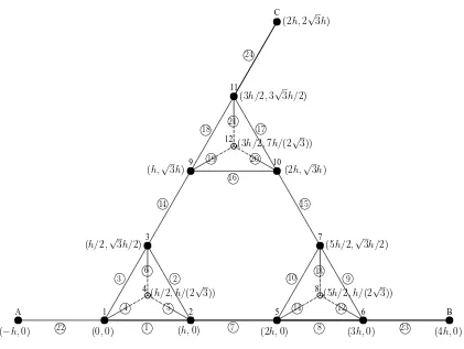
Figure 3: The modified Sierpinski Gasket lattice SG(3,4) at generation level

n = 1. Nodes 1,2 and 3 are the input/output piezoelectric nodes, node 4 is a polymer node, and nodesA(or 5),B(or 6) andC(or 7) are fictitious nodes used to accommodate the boundary conditions. The lattice has 9 elements (circled

1 2 3 4 5 6 7 8 9 10 11 12 A B

(0,0) (h,0) (h/2,√3h/2)

(h/2, h/(2√3))

(2h,0) (3h,0) (5h/2,√3h/2)

(5h/2, h/(2√3)) (h,√3h) (2h,√3h)

(3h/2,3√3h/2)

(3h/2,7h/(2√3))

(−h,0) 1 (4h,0)

2 3 4 5 6 7 8 9 10 11 12 13 14 15 16 17 18 19 20 21 22 23

Figure 4: The modified Sierpinski Gasket lattice SG(3,4) at generation level

n = 2. Nodes A (or 13), B (or 14) and C (or 15) are fictitious nodes used to accommodate the boundary conditions. The lattice has 24 elements (circled

numbers), with two vertices adjacent to each element.

3.1

Transformations of the fundamental basis functions

In this section we will consider transformations of some fundamental basis

func-tions ˆφJ, ˆφK and ˆψI (see Figures 5, 6 and 7) to get basis functions φJ, φK and

x

y

J

B

C

A

D

(0

,

0)

(

√

3

,

0)

(

,

)

(

,

)

(

,

)

x

A

B

C

K

(0

,

0)

(

h,

0)

(

h

₂

,

√

₂

3

h

)

(

h

₂

,

₂

√

h

3

)

Figure 6: Plan view of ˆφK, the fundamental basis function for the polymer vertices.

x

y

I

_D

ˆ

φJ(

2 , 2) = 1 + 2 hb+ 2c+ 4h d+ 4 e= 0, (42)

ˆ φJ( √ 3h 2 , −h

2 ) = 1 +

√

3 2 hb−

h

2c+ 3 4h

2_d+h2

4 e= 0 (43)

and

ˆ

φJ(−

√

3h

2 ,

h

2) = 1−

√

3 2 hb+

h

2c+ 3 4h

2_d+ h2

4 e= 0. (44)

Equations (41) to (44) provide four equations in the four unknowns b, c, d and

e, which give b = 0, c= 0, d=₋3/h2 and e= 5/h2 and substituting these into equation (39) gives

ˆ

φJ(x, y) = 1−

3

h2x 2₊ 5

h2y

2_{. (45)}

Similarly, for the fundamental basis function ˆφK (see Figure 6), we have four nodes, so we need to form an equation with four unknowns, so consider

ˆ

φK(x, y) =a+bx+cy+d(x2+y2). (46)

By applying equation (38), then we get

ˆ

φK(0,0) = a = 0, (47) ˆ

φK(h,0) = hb+h2d= 0, (48)

Equations (48) to (50) provide three equations in the three unknowns b, c and

d, which gives b = 3/h, c = √3/h and d =₋3/h2_{, and substituting these into}

equations (46) gives

ˆ

φK(x, y) =

3

hx+

√

3

h y−

3

h2(x

2_+y2_{). (51)}

Similarly, for the fundamental basis functions ˆψI (see Figure 7), we have two nodes, so consider

ˆ

ψI(x, y) =a+d(x2 +y2). (52)

By applying equation (38), we get

ˆ

ψI(0,0) =a= 1 (53)

and

ˆ

ψI(h,0) = 1 +h2d= 0. (54)

This equation gives d=₋1/h2, and substituting this into equation (52) gives ˆ

ψI(x, y) = 1−

1

h2(x

2_+y2_{). (55)}

Having established the fundamental (canonical) basis functions for each type of

vertex in the lattice we now need to calculate the specific basis functions for each

vertex. In order to do this each fundamental basis functions is mapped onto the

specific vertex by a series of transformations such as a translation, a rotation,

D A

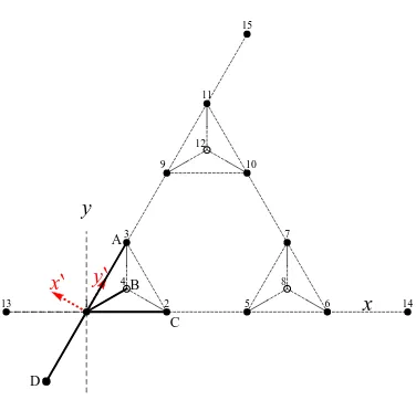
Figure 8: The plan view of the basis function φ2. The coordinate axis x′ lies

along the edge JD in Figure 5.

In Figure 8 the plan view of the basis function centred on vertex 2 at fractal

generation level n = 1 is shown. The form of this basis function is obtained by relating it to the canonical basis function shown in Figure 5 as given by equation

(45) (with respect to the (x′_{, y}′_{) coordinate frame shown in red in Figure 8). To}

transform this plan view of φ2 to the plan view of ˆφJ then we simply need to

transform the (x, y) axis in Figure 8 to the (x′_{, y}′_{) axis in Figure 5. So the first}

step is via a translation of x2 = (h,0) to x′2 = (0,0) (see Figure 9). So, from

equation (45), we have so far

RT(xj) =

y₋yj 

. (57)

x

y

x

¾

y

¾

B C

D

A 1 2

3

4

5 6

7

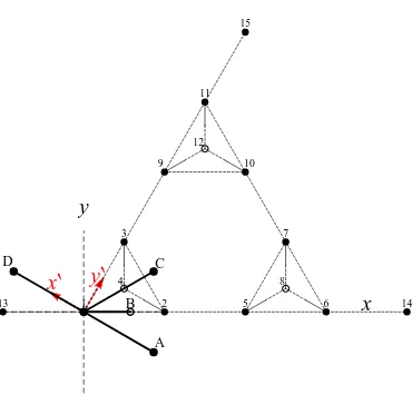
Figure 9: The plan view of φ2, after the first transformation.

The second step in transforming φ2 to ˆφJ is via a reflection in the (y axis) (see

Figure 10). Reflection in the y axis can be obtained by multiplying the basis vectors by the matrix



x

x

A

D

5

1

2

6

Figure 10: The plan view of φ2, after the second transformation.

Then from this plan view ofφ2, the third (final) step in transforming φ2 to ˆφJ is

via a rotation of ₋π/6 (clockwise) (see Figure 11). The anticlockwise rotation by an amount θ is obtained by multiplying the basis vectors by the matrix

Rθ =



 

cosθ ₋sinθ

sinθ cosθ





x

y

x

y

¾ B C A D 1 2 3 4 5 6

Figure 11: The plan view of φ2, after the third (final) transformation.

So, for example, at fractal generation level n = 1,

φ2 = R−π

6 ◦RR◦RT(x2) ˆφJ(x, y) (60)

= R−π

6 ◦RR

ˆ

φJ(x₋x2, y)

= R−π

6

ˆ

φJ(₋x₋x2, y)

= ˆφJ ₋cos(₋π

6)(x+x2)−sin(−

π

6)y,−sin(−

π

6)(x+x2) + cos(−

π

6)y

= ˆφJ −(x+h)

√ 3 2 + 1 2y, 1

2(x+h) +

√

3 2 y

= 1₋ 3

h2 −(x+h)

√ 3 2 + 1 2y 2 + 5 h2 1

2(x+h) +

√

3 2 y

2

Figure 12: The plan view the basis function φ3.

To transform φ3 (see Figure 12) to ˆφJ (see Figure 5) we need a translation of

x3 = (h/2,

√

3h/2) (see Figure 13).

x y

x¾ y ¾

B

A C

D

1 2

3

4

5 6

x

y

x

y

¾

B

C

A D

1 2

3

4

5 6

7

Figure 14: The plan view of φ3, after the second step of transformation.

So,

φ3 = Rπ

2 ◦RT(x3) ˆφJ(x) (62)

= Rπ

2 ◦

ˆ

φJ x₋ h

2, y−

√

3h

2

= ˆφJ ₋y+

√

3h

2 , x−

h

2

= 1₋ 3

h2 −y+

√

3h

2 2

+ 5

h2 x−

h

2 2

Figure 15: The plan view of the basis function ψ6, before transformation.

To transform the basis functionψ6 (see Figure 15) to the canonical basis function

ˆ

ψI (see Figure 7), the first step is a translation ofx6 = (2h,0) (see Figure 16).

x y

x¾ y ¾

D

1 2

3

4

5 6

x

y

x

y

¾

D

1 2

3

4

5 6

7

Figure 17: The plan view of ψ6, after the second (final) step of transformation.

So,

ψ6 = Rπ◦RT(x6) ˆψI(x) (64)

= Rπ_◦ψIˆ (x₋2h, y) = ψIˆ (₋x+ 2h,₋y) = ₋3 + 4

hx−

1

h2x 2

− _h12y

Figure 18: The plan view of the basis function ψ7, before transformation.

To transformψ7(see Figure 18) to ˆψI (see Figure 7), the first step is a translation

of x7 = (h,

√

3h) (see Figure 19).

x y

x¾ y ¾

D

1 2

3

4

5 6

x

y

x

y

¾

D

1 2

3

4

5 6

7

Figure 20: The plan view of ψ7, after the second (final) step of transformation.

So,

ψ7 = R2π

3 ◦RT(x7) ˆψI(x) (66)

= R2π 3 ◦

ˆ

ψI(x₋h, y₋√3h)

= ₋3 + 2

hx+

2√3

h y−

1

h2x 2

− 1

h2y

7 (h, 3h) ₋ 2π/3

Table 1: The related steps of the transformation from φj, j = 1, . . . ,4 and ψj,

j = 5,6,7 to their respective canonical basis function in fractal generation level

n = 1.

A summary of the transformations required for each basis function at fractal

x

y

x

¾

y

¾

_B

A

D

C

1 2

3

4

5 6

7

8

9 10

11

12

13 14

Figure 21: The plan view of the basis function φ75, before transformation.

The above process can then be repeated for fractal generation leveln= 2. Recall that at each generation level the overall length of the lattice remains fixed (L) and the edge length h decreases. As such the canonical basis function given by equation (45) can still be applied here since it will be automatically scaled as

its coefficients depend onh. For example, to transformφ7 (see Figure 21) to ˆφJ

(see Figure 5), the first step is a translation of x7 = (5h/2,

√

x

x

¾

y

¾

B

A

D

C

1 2

4

5 6

8

13 14

Figure 22: The plan view of φ7, after the first transformation.

The second step in transforming φ7 to ˆφJ is via a reflection in the y axis (see

x

y

x

¾

y

¾

B

A

C

D

1 2

3

4

5 6

7

8

9 10

11

12

13 14

Figure 23: The plan view of φ7, after the second transformation.

Then from this plan view of φ7, the third (final) step in transforming φ7 to ˆφJ

x

x

¾

y

¾

B

C

A

D

1 2

4

5 6

8

13 14

Figure 24: The plan view of φ7, after the third (final) transformation.

So,

φ7 = Rπ

2 ◦RR◦RT(x7) ˆφJ(x) (68)

= Rπ

2 ◦RR

ˆ

φJ x−

5h

2 , y−

√

3h

2

= Rπ

2

ˆ

φJ ₋x+5h 2 , y−

√

3h

2

= ˆφJ ₋y+

√

3h

2 ,−x+ 5h

2

= 30₋25

h x+

3√3

h y+

5

h2x 2

− 3

h2y

x

y

x

¾

y

¾

B

A

D

C

1 2

3

4

5 6

7

8

9 10

11

12

13 14

Figure 25: The plan view of the basis function φ9, before transformation.

To transformφ9 (see Figure 25) to ˆφJ (see Figure 5) the first step is a translation

of x9 = (h,

√

x

x

¾

y

¾

_B

A

C

D

1 2

4

5 6

8

13 14

Figure 26: The plan view of φ9, after the first transformation.

x

y

x

¾

y

¾

B

A

C

D

1 2

3

4

5 6

7

8

9 10

11

12

13 14

Figure 27: The plan view of φ9, after the second transformation.

Then from this plan view of φ9, the third (final) step is a rotation of −5π/6

x

x

¾

y

¾

B

C

A

D

Figure 28: The plan view of φ9, after the third (final) transformation.

Hence,

φ9 = R−5π

6 ◦RR◦RT(x9) ˆφJ(x) (70)

= R−5π

6 ◦RR

ˆ

φJ(x−h, y−

√

3h)

= R−5π

6

ˆ

φJ(₋x+h, y₋√3h) = ˆφJ

√

3 2 x−

√

3h

2 +

1 2y−

√

3h

2 , 1 2x−

h

2 −

√

3 2 y+

3h

2

= 1₋ 3

h2

√

3 2 x+

1 2y−

√

3h2

+ 5

h2

1 2x−

√

3 2 y+h

2

x

y

x

¾

y

¾

B

A

D

C

1 2

3

4

5 6

7

8

9 10

11

12

13 14

Figure 29: The plan view of the basis function φ10, before transformation.

To transformφ10(see Figure 29) to ˆφJ (see Figure 5) the first step is a translation

of x10= (2h,

√

x

x

¾

y

¾

B

C

D

1 2

4

5 6

8

13 14

Figure 30: The plan view of φ10, after the first transformation.

x

y

x

¾

y

¾

B

C

A

D

Figure 31: The plan view of φ10, after the second (final) transformation.

So,

φ10 = R−5π

6 ◦RT(x10) ˆφJ(x) (72)

= R−5π

6 ◦

ˆ

φJ(x−2h, y−

√

3h)

= ˆφJ(₋

√

3 2 x+

√

3h+y 2−

√

3h

2 ,− 1

2x+h−

√

3 2 y+

3h

2 )

= 1₋ 3

h2 −

√

3 2 x+

1 2y+

√

3h

2 2

+ 5

h2 −

1 2x−

√

3 2 y+

5h

2 2

= 30₋ 8x₋ 14

√

3

y₋ 1 x2+ 3y2+4

√

3

7 λ(5h

2, 3h

2 ) y axis π/2

8 λ(5h

2 ,

h

2√3) − −

9 λ(h,√3h) y axis ₋5π/6

10 λ(2h,√3h) _{− −}5π/6

11 λ(3h

2 , 3√3h

2 ) − π/2

12 λ(3h

2 , 7h

2√3) − −

13 λ(₋h,0) _{− −}

14 λ(4h,0) ₋ π

15 λ(2h,2√3h) ₋ 2π/3

Table 2: The related steps of the transformation from φj, j = 1, . . . ,12 andψj,

j = 13,14,15 to their respective canonical basis function in fractal generation level n= 2, where λ = 1/3.

A table showing all the transformations required to create the basis functions,

(see Figure 3). The lattice basis functions φ1 at vertex (0,0) (as shown in green

in Figure 32) is connected to node 2 through element 1, nodeAthrough element 7, node 3 through element 3 and node 4 through element 4. The lattice basis

functionsφ2 at vertex (h,0) (as shown in blue in Figure 32) is connected to node

1 through element 1, node B through element 8, node 3 through element 2 and node 4 through element 5. The lattice basis functionsφ3 at vertex (h/2,

√

3h/2) (as shown in blue in Figure 32) is connected to node 1 through element 3, node

2 through element 2, node C through element 9, and node 4 through element 6.

Figure 33: The basis function φ4 at fractal generation level n= 1.

The graph below shows the lattice basis functions ψj wherej = 5,6 and 7 which

are the exterior nodes at fractal generation leveln = 1 (see Figure 3). The lattice basis functionsψ5 at vertex (−h,0) (as shown in red in Figure 34) is connected

to node 1 through element 7. The lattice basis functions ψ6 at vertex (2h,0)

(as shown in blue in Figure 34) is connected to node 2 through element 8. The

lattice basis functions ψ7 at vertex (h,

√

The graph below shows the lattice basis functionsφj wherej = 1,2 and 3 which are some of the interior PZT-5H nodes at fractal generation level n = 2 (see Figure 4). The lattice basis functions φ1 at vertex (0,0) (as shown in green in

Figure 35) is connected to node 2 through element 1, nodeA (that is, node 13) through element 22, node 3 through element 3, and node 4 through element 4.

The lattice basis functions φ2 at vertex (h,0) (as shown in blue in Figure 35)

is connected to node 1 through element 1, node 5 through element 7, node 3

through element 2, and node 4 through element 5. The lattice basis functions

φ3 at vertex (h/2,

√

3h/2) (as shown in blue in Figure 35) is connected to node 1 through element 3, node 2 through element 2, node 9 through element 14, and

node 5 through element 8, nodeB (that is, node 14) through element 23, node 7 through element 9, and node 8 through element 12. The lattice basis functions

φ7 at vertex (5h/2,

√

3h/2) (as shown in blue in Figure 36) is connected to node 5 through element 10, node 6 through element 9, node 10 through element 15,

The graph below shows the lattice basis functions φj where j = 9,10 and 11 which are some of the interior PZT-5H nodes at fractal generation level n = 2 (see Figure 4). The lattice basis functions φ9 at vertex (h,

√

3h) (as shown in green in Figure 37) is connected to node 3 through element 14, node 10 through

element 16, node 11 through element 18, and node 12 through element 19. The

lattice basis functions φ10 at vertex (2h,

√

3h) (as shown in blue in Figure 37) is connected to node 7 through element 15, node 9 through element 16, node 11

through element 17, and node 12 through element 20. The lattice basis functions

φ11 at vertex (3h/2,3

√

through element 11, node 6 through element 12 and node 7 through element

13. The lattice basis functions φ12 at vertex (3h/2,7h/2

√

3) (as shown in red in

Figure 38) is connected to node 9 through element 19, node 10 through element

The graph below shows the lattice basis functions ψj where j = 13,14 and 15 which are the exterior nodes at fractal generation level n = 2 (see Figure 4). The lattice basis functionsψ13at vertex (−h,0) (as shown in green in Figure 39)

is connected to node 1 through element 22. The lattice basis functions ψ14 at

vertex (4h,0) (as shown in blue in Figure 39) is connected to node 6 through element 23. The lattice basis functions ψ15 at vertex (2h,2

√

where (x, y)_∈Ω anda, b, c, d, f and g _∈R_{are coefficients to be determined (see}

Tables 7 and 8 Appendix 11.1) andJ =_{1,2,3_}atn= 1,J =_{1,2,3,5,6,7,9,10,11_} at n = 2 which are the interior PZT-5H nodes, K = _{4_} at n = 1 and

K = _{4,8,12_} at n = 2 which are the polymer nodes and I = _{5,6,7_} at

n = 1, I =_{13,14,15_} atn = 2 which are the exterior PZT-5H nodes. Hence

∇φj(x, y) = 

  

  

(bj + 2djx+gjy, cj+ 2fjy+gjx) j ∈J

(bj + 2djx, cj + 2djy) j _∈K

(76)

MJ

H_ji(n) = Z

e

(aj +bjx+cjy+djx2+fjy2+gjxy)

.(ai+bix+ciy+dix2+fiy2+gixy)

dx

= Z

e

ajai+ (ajbi+aibj)x+ (ajci+aicj)y+ (ajdi+aidj +bjbi)x2

+(ajfi+aifj+cjci)y2+ (ajgi+aigj+bjci+bicj)xy+ (bjdi+

bidj)x3+ (cjfi +cifj)y3+ (bjfi+bifj +cjgi+cigj)xy2+ (bjgi+ bigj +cjdi+cidj)x2y+ (fjgi+figj)xy3+ (djgi+digj)x3y+ (djfi

+difj+gjgi)x2y2+djdix4+fjfjy4dx. (78)

Similarly, for each element (edge) ewhere e_∈MK (which is the set of elements in the interior that are a polymer - piezoelectric mix), then

MK

H_ji(n) = Z

e

aj +bjx+cjy+djx2 +fjy2+gjxy

. ai+bix+ciy+

di(x2+y2)dx

= Z

e

ajai+ (ajbi +aibj)x+ (ajci+aicj)y+ (bibj+ajdi+aidj)x2

+(cicj +ajdi+aifj)y2+ (bicj +bjci+aigj)xy+ (bjdi+bidj)x3+ (cjdi+cifj)y3+ (bjdi+bifj+cigj)xy2 + (cjdi+cidj+bigj)x2y+ digjxy3+digjx3y+ (didj+difj)x2y2+didjx4+difjy4dx. (79)

For the boundary elements e _∈ MI (which is the set of elements that connect to the exterior) note that MIH(n)

ii =MJH

(n)

ii wherei ∈J (corner vertices). For

p(xp, yp)

Figure 41: An isoparametric element (edge) between piezoelectric vertex

p(xp, yp) and polymer vertex q(xq, yq). The fraction of piezoelectric material in this edge is given by ν.

is employed, where s = 0 and s = 1 and dx = h ds (see Figure 40). For the elements that join a piezoelectric node to a polymer node a similar representation

is used but here dx = h/√3ds and the region between s = 0 and s = ν is piezoelectric and that between s = ν and s = 1 is polymer (see Figure 41). Substituting this into equations (78) and (79) gives

H_ji(n) = 

    

    

hR1

0 φjφids ife∈MJ

h √

3

R1

0 φjφids ife∈MK

hR1

0 φjφids ife∈MI.

(81)

Let us start with an interior piezoelectric element (e _∈ MJ), say e = 1 _∈ MJ

= h

Z 1

0

1₋s22

ds. (83)

Similarly,

e=1_H(1)

12 = h

Z 1

0

φ1(hs,0)φ2(hs,0)ds (84)

= h

Z 1

0

1₋s2

2s₋s2

ds

= h

Z 1

0

1₋s2

2₋s

s ds, (85)

where we note that e=1_H(1)

21 =e=1H (1) 12. Also

e=1_H(1)

22 = h

Z 1

0

φ2(hs,0)φ2(hs,0)ds (86)

= h

Z 1

0

2s₋s22

ds

= h

Z 1

0

2₋s2

s2ds. (87)

So for each interior piezoelectric element (e _∈MJ),

MJ

H_ji(n)=h

                 R1

0(s 2

−1)2ds ifj =i=p

R1

0(s

2_{−1)(s−2)s ds if (j =pandi=q) or (j =qandi=p)}

R1

0(s−2)

2_s2_{ds ifj =i=q}

0 otherwise,

(88)

where element e connects nodep to node q. Evaluating these integrals gives

MJ

H_ji(n) = h 30         

16 ifj =i=p

11 if (j =pandi=q) or (j =qandi=p)

e=5_H(1) 24 =

h

√

3 0

φ2(−

h

2 s+h,

h

2√3s)φ4(

−h

2 s+h,

h

2√3s)ds (92) = _√h

3 Z 1

0

1₋s2

2₋s

s ds. (93)

where we note that e=5_H(1)

42 =e=5H (1) 24. Also

e=5_H(1)

44 = h √ 3 Z 1 0

φ4(−

h

2 s+h,

h

2√3s)φ4(

−h

2 s+h,

h

2√3s)ds (94) = _√h

3 Z 1

0

2₋s2

s2_{ds. (95)}

So, for each piezoelectric - polymer element (e_∈MK),

MK

H_ji(n) = _√h 3                  R1

0(s

2₋₁₎2_{ds ifj =i=p}

R1

0(s

2_{−1)(s−2)s ds if (j =pandi=q) or (j =qandi=p)}

R1

0(s−2)

2_s2_{ds ifj =i=q}

0 otherwise.

(96)

That is

MK

H_ji(n) = h 30√3

             

16 ifj =i=p

11 if (j =pandi=q) or (j =qandi=p) 16 ifj =i=q

for c2_K(n)

ji for e ∈ MK, we need to apply equation (23) where MKc2K

(n)

ji =

h/√3 c2

T

Rν

0 ∇φj.∇φids+c 2

P

R1

ν ∇φj.∇φids

and so ν does appear explicitly in that case. For exterior piezoelectric elements (e_∈MI =_{M+1, M+2, M+3_}), let us take the example for one element that is e = 7_∈ MI which is connected between node 1 at (xi, yj) = (0,0) and node 5 at (xj, yj) = (₋h,0) and apply equation (80) to get (x(s), y(s)) = (hs,0). Then from equation (81) we get

e=7_H(1)

11 = h

Z 1

0

φ1(hs,0)φ1(hs,0)ds (98)

= h

Z 1

0

1₋s22

ds. (99)

Similarly, for each exterior piezoelectric element (e_∈MI),

MI

H_ji(n) =h

     R1

0(s

2₋₁₎2_{ds ifj =i=q}

0 otherwise.

(100)

Note that there is only one combination of basis functions in these exterior

piezoelectric elements since the left hand side of equation (31) does not involve

the basis functions at boundary vertices I denoted by ψI. That is

MI

H_ji(n) = h 30     

16 ifj =i=q

0 otherwise

(101)

where q is the corner vertex of the SG(3,4) lattice connected to element e (for

H_ji(2) = h 30                                

H_ji 11 0 0 0 0 0 0 0

0 0 0 0 11 0 0 0

0 0 0 0 0 0 0 0

0 11 0 0 0 0 0 0

0 0 0 0 Hˆ_ji(1) 0 0 0 0

0 0 0 0 0 11 0 0

0 0 0 0 0 0 0 0

0 0 11 0 0 0 0 0

0 0 0 0 0 0 11 0 Hˆ_ji(1)

0 0 0 0 0 0 0 0

0 0 0 0 0 0 0 0

                                . (103)

Similarly for e_K(n)

ji we can write equation (37)

MJ

K_ji(n) = c2

Z

e

(bj + 2djx+gjy, cj+ 2fjy+gjx).(bi + 2dix+giy, ci+ 2fiy+gix)

dx

= c2

Z

e

bjbi+ 2(bjdi+bidj)x+ (bjgi+bigj)y+ 4djdix2+gjgiy2

+2(djgi+digj)xy+cjci+ (cjgi+cigj)x+ 2(cjfi+cifj)y+gjgix2

+4fjfiy2+ 2(fjgi+figj)xy

= c2

Z

e

bibj + 2(djbi+dibj)x+ 4didjx2+cicj + 2(dicj +djci)y

+4didjy2dx. (105)

By using the definition of cthat in equation (23) and using equation (80) then we can write equation (37) as

K_ji(n)=            hc2 T R1

0 ∇φj.∇φids ife∈MJ

h √ 3 c 2 T Rν

0 ∇φj.∇φids+c 2

P

R1

ν ∇φj.∇φids

ife_∈MK hc2

T

R1

0 ∇φj.∇φids ife∈MI,

(106)

where ν is a parameter indicating the volume fraction of piezoelectric material in edge e. For e_∈MJ,

MJ

K_ji(n)=hc2_T

                 52 h2 R1 0 s

2_{ds ifj =i=p}

−44

h2

R1

0 s(s−1)ds if (j =pandi=q) or (j =qandi=p) 52

h2

R1

0(s−1)2ds ifj =i=q

0 otherwise.

(107)

That is

MJ

K_ji(n) = 2 3hc

2 T                 

26 ifj =i=p

11 if (j =pandi=q) or (j =qandi=p) 26 ifj =i=q

0 otherwise.

MK

K_ji(n) = 2 3hc

2 T                        

2√3 ν3₊c2P

c2

T(1−ν 3₎

ifj =i=p

√

3 ν2_(2ν−3)− c2P

c2

T(ν−1)

2_{(1 + 2ν)}

if (j =pandi=q) or (j =qandi=p) 2√3 ν(ν2 _{−3ν+ 3)−} c2P

c2

T(ν−1) 3

ifj =i=q

0 otherwise.

(110)

For e_∈MI,

MI

K_ji(n) =hc2_T

     52 h2 R1 0 s

2_{ds ifj =i=q}

0 otherwise.

(111)

That is

MI

K_ji(n)= 2 3hc

2 T     

26 ifj =i=q

0 otherwise.

(112)

Assembling the full matrix in equation (37) gives, for generation level n= 1

K_ji(1) = 2 3hc

2 T         

D 11 11 R

11 D 11 R

11 11 D R

R R R E

         = 2

3hc

2

TKˆ

(1)

K_ji(2)= 2 3hc

2 T                                    

0 0 0 0 0 0 0 0

ˆ

K_ji(1) 11 0 0 0 0 0 0 0

0 0 0 0 11 0 0 0

0 0 0 0 0 0 0 0

0 11 0 0 0 0 0 0

0 0 0 0 Kˆ_ji(1) 0 0 0 0

0 0 0 0 0 11 0 0

0 0 0 0 0 0 0 0

0 0 11 0 0 0 0 0

0 0 0 0 0 0 11 0 Kˆ_ji(1)

0 0 0 0 0 0 0 0

0 0 0 0 0 0 0 0

                                    . (114)

Combining equations (102) and (113) gives equation (35) as

A(1)_ji =h

        

α β β _P β α β _P β β α _P

P P P θ

        

=hAˆ(1)_ji , (115)

whereα= (q2_{/30) 48 + (16/}√₃₎

+ (2/3) 78 + 2√3 ν3_{+ (c}2

P/c2T)(1−ν3)

, β = (11/30)q2_{+22/3,P = (q}2_/30)(11/√_3)+(2/3) √_{3 ν}2_{(2ν−3)−(c}2

P/c2T)(ν−1)2(1+

2ν)

,and θ= (q2_/30)(48/√_{3) + (2/3) 6}√_{3 ν(ν}2_{−3ν+ 3)−(c}2

P/c2T)(ν−1)3

             

0 0 0 0 0 0 0 0

0 0 β 0 0 0 0 0

0 0 0 0 0 0 β 0 Aˆ(1)_ji

0 0 0 0 0 0 0 0

0 0 0 0 0 0 0 0

             

A similar treatment, by using the definition of c that in equation (23), can be given to equation (34) to give m= (N + 1)/2

b(_jn)=                       

−(R

eM+1(q

2_ψ

N+2φj +h2∇ψN+2.∇φj)dx)UA, j = 1

−(R

eM+2(q

2_ψN

+3φj +h2∇ψN+3.∇φj)dx)UB, j=m = (N + 1)/2

−(R

eM+3(q

2_ψN

+4φj +h2∇ψN+4.∇φj)dx)UC, j =N

0 otherwise.

b(_jn)=hη               

UB, j =m

UC, j =N

0 otherwise

(118)

where

η= 2 3 −

11 30q

2_{. (119)}

For generation level n = 1,

b(1)_j =h(2 3 − 11 30q 2₎                       

UA, j = 1

UB, j = 2

UC , j= 3

0 otherwise

, (120)

and for generation level n= 2,

b(2)_j =h(2 3− 11 30q 2₎                       

UA, j = 1

UB , j= 6

UC , j = 11

0 otherwise

. (121)

4

A Homogenised Model of the Transducer

is black and the polymer is white. It clearly shows the regularity in the structure

and the reliance on a single length scale.

operating characteristics that one would obtain from a conventional (i.e.

non-fractal) 1-3 composite transducer as illustrated in Figure 42. The constitutive

relations for the individual phases have a compact form, within the ceramic (E) phase, and within the polymer (P) phase [35, 34, 15]. From equation (1), and due to the properties of PZT-5H (see Appendix), we get

T11 =T12 =T21=T22 =T33= 0, (122)

and

T13=T31 =c1313S13+c1331S31−e113E1. (123)

That is

T5 =c55(S13+S31)−e15E1, (124)

and, using equation (3), since from equation (9) u1,3 = 0, then

T5 =c44u3,1−e24E1, (125)

So we rewrite equations (125) and (127), for the piezoelectric phase as

T₅E =cE₄₄u₃E_,1−e24E1E (128)

and

T₄E =cE₄₄uE_3,2−e24E2E. (129)

Similarly, for polymer phase we get

T₅P =cP₄₄uP_3,1, (130)

and

T₄P =cP₄₄uP_3,2, (131)

since there is no piezoelectric effect in the polymer phase. From equation (2) we

get for the piezoelectric phase

D1E =e24uE3,1+εE11E1E, (132)

and

D₂E =eE₂₄uE_3,2+εE₁₁E₂E, (133) and for the polymer phase we get

D₁P =εP₁₁E₁P, (134)

and

D₂P =εP₁₁E₂P, (135)

whereDE

3,DP3 are zero. We assume that any movement (strain) in the polymer

That is

v(n) =

3

2(3n−1) + 3n− 1 2ν 3

2(3n−1) + 3

n−12

(139)

and ¯v(n) _{= 1−v}(n) _{is the volume fraction of polymer, where ν is the volume}

fraction of ceramic in the edges adjacent to the degree three vertices as detailed

in section 3 and in equation (106) (see Figure 3, 4). For example at generation

level (n = 1) if ν = 1 then v = 1 and if ν = 0 then v = 3/(3 +√3). Assuming the electric fields are similarly averaged then

¯

E1 =vE1E + ¯vE1P, (140)

and

¯

E2 =vE2E + ¯vE2P. (141)

Assuming that the stresses in each phase are equal then

¯

T4 =T4E =T4P (142)

and

¯

and

¯

D2 =D2E =DP2. (145)

From the symmetry of the SG(3,4) lattice (see Figure 44) then we have

¯

u3,2 = ¯u3,1 = ¯u, (146)

since uE

3,2 = uE3,1 = uE, and uP3,2 = uP3,1 = uP. We take the electric fields to be

the same in both phases, namely,

¯

E1 = ¯E2 = ¯E, (147)

since EE

1 =E2E =EE, and E1P =E2P =EP. Also

¯

T4 = ¯T5 = ¯T , (148)

and

¯

D1 = ¯D2 = ¯D. (149)

From equations (142), (148), (146) and (147) we can write equation (129) as

¯

T =cE₄₄uE ₋e24EE, (150)

and from equations (144), (149), (146) and (147) we can write equation (132) as

¯

D=e24uE +εE11EE. (151)

From equation (152) we get

uP = T¯

cP

44

, (156)

and from equation (153) we get

EP = D¯

εP

11

. (157)

Hence, from equations (154) and (156) we get

uE = 1

v( ¯S−v¯

¯

T cP

44

), (158)

and from equations (155) and (157) we get

EE = 1

v( ¯E−v¯

¯

D εP

11

). (159)

Substituting equations (158) and (159) into equation (150) gives

¯

T =cE₄₄1

v( ¯S−¯v

¯

T cP

44

)₋e24

1

v( ¯E−v¯

¯

D εP

11

). (160)

That is

¯

T 1 + vc¯

E 44 vcP = c E 44

v S¯− e24

v E¯+

¯

ve24

That is

¯

D 1 + ¯vε

E

11

vεP

11

= e24

v S¯−

¯

ve24

vcP

44

¯

T + ε

E

11

v E.¯ (163)

Hence,

¯

D= ε

P

11e24

vεP

11+ ¯vεE11

¯

S₋ ve¯ 24ε P

11

cP

44(vεP11+ ¯vεE11)

¯

T + ε

P

11εE11

vεP

11+ ¯vεE11

¯

E. (164)

That is

¯

D= ε

P

11e24

¯

ε∗ S¯−

¯

ve24εP11

cP

44ε¯∗

¯

T + ε

P

11εE11

¯

ε∗ E,¯ (165)

where ¯ε∗ _=vεP

11+ ¯vεE11. Putting this into equation (161) gives

¯

T 1 + vc¯

E 44 vcP 44 = c E 44

v S¯− e24

v E¯+

¯

ve2 24

vε¯∗ S¯−

¯

v2_e2 24

vcP

44ε¯∗

¯

T + ¯ve24ε

E

11

vε¯∗ E¯ (166)

that is

¯

T 1 + vc¯

E

44

vcP

44

+ v¯

2_e2 24

vcP

44ε¯∗

= c E 44 v + ¯ ve2 24

vε¯∗

¯

S+ ve¯ 24ε

E

11

vε¯∗ − e24 v ¯ E, (167) and so ¯

T vcP₄₄ε¯∗_{+ ¯vc}E

44ε¯∗+ ¯v2e224

= cE₄₄cP₄₄ε¯∗_{+ ¯vc}P

44e224

_¯

S+ ¯vcP₄₄e24ε11E −cP44e24ε¯∗

_¯

E.

(168)

That is

¯

T = ¯c44S¯−e¯24E,¯ (169)

since ¯c44= cE44cP44ε¯∗+¯vcP44e224

/ vcP

44ε¯∗+¯vcE44ε¯∗+¯v2e224

and ¯e24 = cP44e24vεP11

/ vcP

44ε¯∗+

¯

vcE

44ε¯∗ + ¯v2e224

. Substituting this into equation (165) gives

where ¯ε11= (εP11εE11)/ε¯∗+ (¯ve24εP11e¯24)/(cP44ε¯∗). We then have

¯

E = D¯ ¯

ε11 −

¯

e24

¯

ε11

¯

S, (174)

and so we can rewrite equation (169) as

¯

T = ¯c44S¯−e¯24

¯

D

¯

ε11 −

¯

e24

¯

ε11

¯

S

. (175)

That is

¯

T = ¯cT₄₄S¯₋ζ¯D,¯ (176)

where ¯cT

44 = ¯c44+ ¯e224/ε¯11 and ¯ζ = ¯e24/ε¯11. The specific acoustic impedance of

the composite is then [33],

¯

ZT = q

¯

cT

44ρT¯ (177)

where ¯ρT =vρE_+¯vρP _{is the average density, and the longitudinal velocity is [33],}

¯

cT = s

¯

cT

44

¯

ρT. (178)

In order to calculate the transmission sensitivity, consider the circuit shown in

Figure 43. The current across the transducer ¯I is given by [29]

¯

ZE = 1

qC¯0Z0

1₋ ζ¯

2_C¯ 0

2qZT¯ ( ¯KFTF¯ + ¯KBTB¯ )

, (180)

where ¯TF = 2 ¯ZT/( ¯ZT +ZL) and ¯TB = 2 ¯ZT/( ¯ZT +ZB) are non-dimensional transmission coefficients, ¯KF and ¯KB are also non-dimensional and are given by

¯

KF = (1−e−

qτ¯_)(1−RBe¯ −qτ¯₎

(1₋R¯FR¯Be−2qτ¯)

(181)

and

¯

KB =

(1₋e−qτ¯_)(1−R¯

Fe−qτ¯)

(1₋RF¯ RBe¯ −2qτ¯₎ (182)

where ¯RF = ( ¯ZT ₋ZL)/( ¯ZT +ZL) and ¯RB = ( ¯ZT ₋ZB)/( ¯ZT +ZB) are non-dimensionalised reflection coefficients and ¯τ = L/cT¯ is the wave transit time across the device. Note that the capacitance of the device is given by ¯C0 =

Arε¯11/L. The non-dimensionalised transmission sensitivity ¯ψ is [14]

¯

ψ(f) =F¯

V

/ζ¯C¯0 =−

aAF¯ λ¯KF¯

2 ¯C0

1₋ ζ¯

2_λ¯_{( ¯KFTF + ¯KBTB)}

2qZT¯

−1

, (183)

where ¯λ= ¯C0/(1 +qC¯0b) and ¯AF = 2ZL/(ZL+ ¯ZT) are dimensionless constants.

The non-dimensionalised reception sensitivity ¯φ is [13]

¯

φ=V¯

F

(¯e24L) =

−ζTF¯ KF¯ H¯¯e

24L

qZ¯T

1₋ ζ¯

2_H¯_{( ¯KFTF + ¯KBTB)}

2q2_Z¯

TZE

₋1

, (184)

where ¯H =qC¯0b/(1 +qC¯0b).Having derived expressions for the main operating

characteristics of a homogenised device these will be used to compare with the

where uL is the displacement of the load material, ρL is the density and YL is the shear modulus. That is

∂2_uL

∂t2 =

YL ρL

∂2_uL

∂x2

L

(186)

and so, nondimensionalising in a similar fashion to equation (24), gives

∂2uL ∂θ2 =

hcL

cT

2∂2uL

∂x2

L

(187)

wherecL is the wave speed in the load (c2

L =YL/ρL). Taking Laplace transforms

as was done in equation (25) gives

∂2_uL¯

∂x2

L −

qcT

hcL

2 ¯

uL= 0. (188)

Hence, the displacement in the load is

¯

uL=ALe(−qcTxL/hcL)+BLe(qcTxL/hcL), (189)

whereAL andBL are constants. Similarly the displacement in the backing layer (subscript B) is given by

¯

uB =ABe(−qcTxB/hcB)

+BBe(qcTxB/hcB)

Z P ZP

Z0 Backing

Material

Vs

Mechanical Load Sierpinski Gasket

Figure 43: Physical layout of the fractal transducer.

whereABandBBare constants andcBis the wave speed in the backing material.

As the backing layer is highly attenuative it is assumed that there is only a wave

travelling away from the piezoelectric layer (SG(3,4)) interface (xB = 0) in the

direction of increasing xB, and so we set BB = 0. Continuity of displacement

at the transducer-mechanical load interface and the symmetry of the SG(3,4) lattice give

UA = ¯uB(0) =AB, (191)

x2

Figure 44: The line of symmetry given by x1 =x2

F =Ar¯cT₄₄S¯₋ζ¯DAr.¯ (194)

By applying an electrical charge ¯Q at one of the transducer-electrical load in-terfaces then Gauss’ law gives ¯D= ¯Q/Ar. Since ¯S=∂u/∂x¯ , then

F =Ar¯cT₄₄∂u¯

∂x −ζ¯Q.¯ (195)

So from the continuity of force we get FT(¯um) = FL(¯u∂Ω) = FL(xL = 0). That

is, from equation (189),

Ar¯cT44

(UB−Um)

h −ζ¯Q¯ =ArYL

qc

T hcL

(₋AL+BL), (196)

and so

At each generation level of the Sierpinski gasket transducer the ratio of the

cross-sectional area of each edge to its length is denoted by ξ = Ar/h. The overall extent of the lattice (L) is fixed and so the length of the edges will steadily decrease and, by fixing ξ, the cross-sectional area will also decrease as the fractal generation level increases. Hence, equation (197), and its equivalent

at the front face of the transducer, can be written

U1−UA−

¯

ζQ¯

¯

cT

44ξ

= ZB_¯¯

ZT q(−AB), (198)

UB−Um−

¯

ζQ¯

¯ cT 44ξ = ZL ¯¯ ZT

q(₋AL+BL). (199)

From equations (191) and (198) we have thatUA=γ1U1+δ1 and from equations

(192),(193) and (199) we have

UB =γmUm+δm =UC =γNUN +δN, (200)

where γj =       

(1₋qZB ¯ ¯

ZT)

−1_{, j = 1}

(1₋qZL ¯ ¯

ZT)

−1_{, j =m orN}

(201) and δj =       

−_¯cζ¯TQ¯ 44ξ

1₋qZB ¯ ¯

ZT

−1

, j = 1

1₋qZL ¯ ¯

ZT

−1 _¯

ζQ¯

¯

cT

44ξ −2ALq

ZL

¯ ¯

ZT

, j =morN.

(202)

ˆ

Bji(n) =

                      ... ... ... 0 0 ¯ γm 0 0 . .. ... ...

... . .. 0 0

0 _{· · · · · ·} 0 ¯γN

                      . (206) That is

F_ji(n)Ui = ¯δj, (207)

and so

Ui =G(_jin)δj,¯ (208)

where

G(_jin) = F_ji(n)−1

= ˆA(_jin)₋Bˆ_ji(n)−1

(209)

U_j(n) =G(_jn₁)δ¯1+G(jmn)δm¯ +G

(n)

jNδN¯ . (210)

In particular we will be interested in U₁(n), Um(n) and U_N(n) and so we only need

to be able to calculate the pivotal Green’s functions G(_ijn), i, j _{∈ {}1, m, N_}. If

1 b e m

d

r

q z

N

Figure 45: Three Sierpinski Gasket lattices of generation leveln₋1 are connected by the edges in bold (b, e),(d, r) and (q, z)

to create the Sierpinski Gasket

lattice at generation level n.

we temporarily ignore matrix ˆB in equation (209) (this matrix originates from consideration of the boundary conditions) then, due to the symmetries of the

SG(3,4) lattice (and hence in matrix A(n)_{), we have}

ˆ

the nondimensionalised natural frequency, ˆω(n) _{is the nondimensionalised}

angu-lar frequency and f(n) _{(and ω}(n)_{) are the dimensionalised equivalents. In order}

to use the renormalisation approach detailed below then we setq=q(n)_=q(n+1)_.

This simply means that the output from the renormalisation methodology (and

hence the electrical impedance and transmission/reception sensitivities) at a

given q (fixed) is then that quantity at frequency f(n) _{at generation level n. So}

when comparing outputs at different generation levels one must ensure that the

frequency is scaled appropriately (by (cT/h(n)₎−1_{) when re-dimensionalising. An}

iterative procedure can be developed from equation (35) which can be written

as

ˆ

A(_jin) = 8₅q2In₋T(n) (215)

where

T(n) =βR(n)₋4In, (216)

R =  

−1 0 ₋1

−1 ₋1 0   

, (218)

and (see Figure 45)

V(n) = 

  

  

−1 if (h, k)_{∈ {}(b, e),(d, r),(q, z),(e, b),(r, d),(z, q)_}

0 otherwise

. (219)

So, using equations (215) and (216), we can write equation (213) as

ˆ

G(n) = 8₅q2In₋T(n)−1

= (8

5q

2_{+ 4)I}

n−βR(n)

−1

. (220)

Hence,

( ˆG(n+1))−1 _{= (}8 5q

2_{+ 4)In}

+1−βR(n+1). (221)

Since ¯G(n) _{is a block-diagonal matrix then}

( ¯G(n))−1 _{= A}ˆ(n)

= 8₅q2_In−T(n)

= 8

5q 2_In

+1−T¯(n)

= 8₅q2In+1−(βR¯(n)−4 ¯In)

= (8₅q2+ 4)In+1−βR¯(n). (222)

Now

ij

(209),(215) and (216)

(G(n))−1 _{= Aˆ}(n)

−Bˆ(n)

= (8 5q

2_In

−T(n))₋Bˆ(n)

= 8₅q2In₋(βR(n)₋4In)₋Bˆ(n)

= (8 5q

2_{+ 4)In}

−βR(n)₋Bˆ(n). (225) Now, from equation (220)

In = Gˆ(n)( ˆG(n))−1

= Gˆ(n) (8₅q2+ 4)In₋βR(n)₋Bˆ(n)+ ˆB(n)

.

From equation (225) then,

In = Gˆ(n) (G(n))−1_{+ ˆB}(n)

= Gˆ(n) (G(n))−1_{+ ˆB}(n)_G(n)_(G(n)₎−1

= ( ˆG(n)+ ˆG(n)Bˆ(n)G(n))(G(n))−1_{. (226)}

ˆ

G(_ijn+1) = ¯G(_ijn)+X

h,k

βG¯(_ihn)V_hk(n)Gˆ(_kjn+1). (228)

The system of linear equation in ˆG(_ijn+1) will create the renormalisation recursion relationships for the pivotal Green’s functions. However, these recursions do not

include the boundary conditions. Since the subgraphs of Figure 1 only connect

to each other at the corners, it will transpire that the recursions in equation (228)

only involve two pivotal Green’s functions, namely, to-corner and

corner-to-same-corner; the so called input/output nodes. To proceed, we now need to

determine ˆx and ˆy as defined in equations (211) and (212). Using equations (219) and (228) we get

ˆ

G(₁₁n+1) = G¯(₁₁n)+X

h,k

βG¯(₁n_h)V_hk(n)Gˆ(_kn₁+1)

= Gˆ(₁₁n)+βG¯₁(n_d)V_dr(n)Gˆ_r(n₁+1)+βG¯(₁n_b)V_be(n)Gˆ(_en₁+1)

= Gˆ(₁₁n)₋βGˆ₁(n_N)Gˆ(_rn₁+1)₋βGˆ₁(n_m)Gˆ(_en₁+1).

That is

ˆ

X = ˆx₋2βyˆGˆ(en1+1), (229)

since we know from equation (219) that V_dr(n) = V_be(n) = ₋1 and by symmetry ¯

G₁(n_d)= ˆG(₁n_N), Gˆ(₁n_N)= ˆG₁(n_m) and ˆG(_rn₁+1) = ˆG(_en₁+1). Similarly,

ˆ

G(_en₁+1) = G¯(_en₁)+X

h,k

βG¯(_ehn)V_hk(n)Gˆ(_kn₁+1)

ˆ

G_b(n₁+1)= ˆy₋βGˆ_e(n₁+1)(ˆx+ ˆy), (231) since ˆG(_rn₁+1) = ˆG(_en₁+1). Finally,

ˆ

G(_zn₁+1) = G¯(_zn₁)+X

h,k

βG¯(_zhn)V_hk(n)Gˆ(_kn₁+1)

= βG¯(_zrn)V_rd(n)Gˆ(_dn₁+1)+βG¯(_zzn)V_zq(n)Gˆ(_qn₁+1)

= ₋βGˆ(mn1)Gˆ (n+1)

b1 −βGˆ(mmn) Gˆ

(n+1)

z1 .

Therefore

ˆ

G(_zn₁+1) =₋βyˆGˆ(_bn₁+1)₋βxˆGˆ(_zn₁+1), (232) since ˆG(_dn₁+1) = ˆG(_bn₁+1) and ˆG(_qn₁+1) = ˆG(_zn₁+1). Equations (229) to (232) provide four equations in the four unknows ˆX,Gˆ(_en₁+1),Gˆ_b(n₁+1) and ˆG(_zn₁+1). Rearranging equation (229) gives (for ˆy₆= 0, β ₆= 0)

ˆ

G(_en₁+1) = xˆ−Xˆ

2βyˆ , (233)

and substituting this into equation (231) gives

ˆ

G(_bn₁+1) = ˆy+ (ˆx+ ˆy)Xˆ −xˆ 2ˆy