O perators a nd & M atrices www.ele-math.com
VARIATIONAL PRINCIPLES FOR SELF–ADJOINT OPERATOR FUNCTIONS ARISING FROM SECOND–ORDER SYSTEMS
BIRGITJACOB, MATTHIAS LANGER ANDCARSTENTRUNK
Submitted to Operators and Matrices
Abstract. Variational principles are proved for self-adjoint operator functions arising from vari-ational evolution equations of the form
hz(t),¨ yi+d[z(t),y] +˙ a0[z(t),y] =0.
Here a0 and d are densely defined, symmetric and positive sesquilinear forms on a Hilbert spaceH. We associate with the variational evolution equation an equivalent Cauchy problem corresponding to a block operator matrixA , the forms
t(λ)[x,y]:=λ2hx,yi+λd[x,y] +a0[x,y],
where λ ∈C and x,y are in the domain of the form a0, and a corresponding operator fam-ily T(λ). Using form methods we define a generalized Rayleigh functional and characterize the eigenvalues above the essential spectrum of A by a min-max and a max-min variational
principle. The obtained results are illustrated with a damped beam equation.
1. Introduction
Variational principles are a very useful tool for the qualitative and numerical inves-tigation of eigenvalues of self-adjoint operators and operator functions. For instance, the eigenvalues λ1 ≤λ2≤. . . below the essential spectrum of a self-adjoint operator
A that is bounded from below and has domain D(A) can be characterized using the
Rayleigh functional
p(x) = hAx,xi
hx,xi , x∈D(A),x6=0, via a min-max principle or a max-min principle:
λn= min L⊂D(A)
dimL=n
max
x∈L\{0} p(x) = maxL⊂H
dimL=n−1
min
x∈D(A)\{0} x⊥L
p(x).
Variational principles were first introduced by H. Weber, Lord Rayleigh, H. Poincar´e, E. Fischer, G. Polya, and W. Ritz, H. Weyl, R. Courant (see, e.g. [4, 7, 20], and the references therein).
Mathematics subject classification(2010): 47A56, 49R05, 47A10.
In this article we investigate variational principles for self-adjoint operator func-tions arising from variational evolution equafunc-tions of the form
hz¨(t),yi+d[z˙(t),y] +a0[z(t),y] =0. (1.1) Here a0 with domain D(a0) and d with domain D(d)⊃D(a0) are densely defined, symmetric and posivite sesquilinear forms on a Hilbert space H satisfying(F1)–(F3), see Section 3. With this variational evolution equation we associate a Cauchy problem
z˙
˙
w
=A
z
w
,
z (0) w(0)
=
z
0
w0
(1.2)
on D(a0)×H in such a way that the solutions of (1.1) equal the first component of the solutions of (1.2). For λ∈C we define the sesquilinear form
t(λ)[x,y]:=λ2hx,yi+λd[x,y] +a0[x,y] (1.3) with domainD(t(λ)):=H1
2 :=D(a0). We identify a discΦγ0 ⊂Cwhich is the largest
disc around zero with an empty intersection with the essential spectrum of A . For
λ ∈Φγ0 we show that the form t(λ) is closed and sectorial and that the corresponding
operator T(λ) is m-sectorial. Moreover, on Φγ0 the spectrum (point spectrum) of A
and the spectrum (resp. point spectrum) of T coincide.
In [7] R. J. Duffin proved a variational principle for eigenvalues of a quadratic ma-trix polynomial, which was generalized in various directions to more general operator functions; see, e.g. the references in [9] and [19]. In [9] such a variational principle was proved for eigenvalues of operator functions whose values are possibly unbounded self-adjoint operators. Here we adapt this variational principle from [9] to our situation. Using the form t(λ) we introduce a slightly more general definition of a generalized
Rayleigh functional and we show that the variational principle generalizes to this situa-tion. In particular, for a fixed x∈H1
2\ {0}, denote the two real solutions (if they exist)
of the quadratic equation
t(λ)[x,x] =0
by p−(x) and p+(x) such that p−(x)≤ p+(x) is satisfied and set p+(x) :=−∞, p−(x):=∞ if there are no real solutions. Then the function p+ plays the role of a
generalized Rayleigh functional in our main theorem, which yields variational prin-ciples for the real eigenvalues of A or, what is equivalent, of T. These variational
principles hold in certain real intervals ∆above the essential spectrum of A in the disc Φγ0 with the property that ∆ does not contain values of p−. In ∆ the spectrum of A
is either empty or consists only of a finite or infinite sequence of isolated semi-simple eigenvalues of finite multiplicity of A . Moreover, we show that these eigenvalues
λ1≥λ2≥ ···, counted according to their multiplicities, satisfy
λn= max L⊂H1/2
dimL=n
min
x∈L\{0} p+(x) = minL⊂H
dimL=n−1
sup
x∈H1/2\{0}
x⊥L
and, if N<∞, we show for n>N that sup
L⊂D
dimL=n
min
x∈L\{0} p+(x)≤inf∆ and Linf⊂H
dimL=n−1 sup
x∈D\{0} x⊥L
p+(x)≤inf∆.
A major application of this variational principle is a quite general interlacing principle which is the second main result of this article: if the stiffness operatorA0 decreases and the damping operator D increases, then the corresponding nth eigenvalue decreases compared with the nth eigenvalue of the unchanged system. We illustrate the obtained results with an example where we consider a beam equation with a damping such that
A0 corresponds to the fourth derivative on the interval (0,1) (with some appropriate boundary conditions) and the damping D equals −ddxdddx with some smooth function
d (and some boundary conditions).
We proceed as follows. The variational principle obtained in [9] is adapted to the setting of this paper in Section 2. Section 3 is devoted to general properties of the class of second-order systems studied in this paper. The main results of this paper are proved in Section 4. In particular, we study the form (1.3) and their relation to the op-erator matrix A and the operator function T(λ). On a disc Φγ0 around zero, t(λ) is a
closed sectorial form and the spectrum (point spectrum) of A and the spectrum (point
spectrum) of T coincide. Further, the variational principles for A are presented in
Theorem 4.8. As an application of the variational principle we show interlacing prop-erties of eigenvalues of two different second-order problems with coefficients which satisfy a specific order relation. Finally, in Section 5 we apply the obtained results to a damped beam equation.
Throughout this paper we use the following notation. For a self-adjoint operator
S and an interval I we denote by LI(S) the spectral subspace of S corresponding to I. A closed, densely defined operator in H is calledFredholm if the dimension of its kernel and the (algebraic) co-dimension of its range are finite. Theessential spectrum
of a closed, densely defined operator S is defined by
σess(S):=λ ∈C|S−λI is not Fredholm .
A closed, densely defined operator T is calledsectorialif its numerical range is con-tained in a sector {z∈C|Rez≥z0,|arg(z−z0)| ≤θ} for somez0∈R andθ∈[0,π2). A sectorial operator T is calledm-sectorialif λ ∈ρ(T) for some λ with Reλ <z0; see, e.g. [15, §V.3.10]. For a sesquilinear form a[·,·] with domain D(a) the
corre-sponding quadratic form is defined bya[x]:=a[x,x], x∈D(a). A form is called secto-rialif its numerical range is contained in a sector {z∈C|Rez≥z0, |arg(z−z0)| ≤θ} for some z0∈R and θ ∈[0,π2); see, e.g. [15,§V.3.10].
2. A general variational principle for self-adjoint operator functions
For the rest of this section let ∆⊂R be an interval with
a=inf∆ and b=sup∆, −∞≤a<b≤∞, (2.1) and let Ω be a domain in C such that ∆⊂Ω. On Ω we consider a family of closed,
densely defined operators T(λ), λ ∈Ω, in a Hilbert space H with inner product h·,·i,
where T(λ) has domain D(T(λ)). In the following we shall assume that either T(λ)
or −T(λ) is an m-sectorial operator forλ ∈Ω. Under this assumption the sesquilinear
form hT(λ)·,·i is closable for λ ∈Ω, and we denote the closure by t(λ)[·,·] with
domain D(t(λ)) and set t(λ)[x]:=t(λ)[x,x], which is the corresponding quadratic
form. Recall (see, e.g. [15, §VII.4]) that T := (T(λ))λ∈Ω is called a holomorphic family of type(B) if T(λ) is m-sectorial for λ ∈Ω, the domain D(t(λ)) of the closed
quadratic form t(λ) is independent of λ, which we denote by D, and λ 7→t(λ)[x] is
holomorphic on Ω for every x∈D.
We suppose that one of the following two conditions is satisfied.
(I) Let Ω be a domain in C and ∆⊂Ω∩R an interval with endpoints a, b as in
(2.1). The family (T(λ))λ∈Ω is a holomorphic family of type (B), T(λ)is self-adjoint for λ ∈∆ and there exists ac∈∆ such that dimL(−∞,0)(T(c))<∞.
(II) Let Ω be a domain in C and ∆⊂Ω∩R an interval with endpoints a, b as in (2.1). The family (−T(λ))λ∈Ω is a holomorphic family of type (B), T(λ) is
self-adjoint forλ ∈∆and there exists a c∈∆such that dimL(0,∞)(T(c))<∞.
Note that under assumption (I) for λ ∈∆ the operators T(λ) are self-adjoint and
sec-torial, and, hence, bounded from below. Similarly, under assumption (II), the operators
T(λ) are bounded from above for λ ∈∆. The condition dimL(−∞,0)(T(c))<∞ is
equivalent to the fact that σ(T(c))∩(−∞,0) consists of at most a finite number of
eigenvalues of finite multiplicities.
Before we formulate the second set of assumptions, let us recall the following definitions. Thespectrumof the operator function T is defined as follows:
σ(T):=λ ∈Ω|T(λ)is not bijective fromD(T(λ))ontoH =λ ∈Ω|0∈σ(T(λ)) .
Similarly, theessential spectrumof the operator function T is defined as
σess(T):=λ ∈Ω|T(λ)is not Fredholm =λ ∈Ω|0∈σess(T(λ)) . A number λ ∈Ω is called an eigenvalue of the operator function T if there exists an x∈D(T(λ)), x6=0, such that T(λ)x=0. The point spectrum is the set of all
eigenvalues:
σp(T):=λ ∈Ω| ∃x∈D(T(λ)),x6=0,T(λ)x=0
where σp(T(λ)) denotes the point spectrum of the operator T(λ) for fixed λ ∈Ω. Thegeometric multiplicityof an eigenvalue λ of the operator function T is defined as the dimension of kerT(λ).
In addition to (I) or (II) we shall assume that one of the following two conditions
(&), (%) is satisfied.
(&) For every x∈D\ {0} the function λ 7→t(λ)[x] isdecreasing at value zeroon ∆, i.e. if t(λ0)[x] =0 for some λ0∈∆, then
t(λ)[x]>0 forλ ∈(−∞,λ0)∩∆,
t(λ)[x]<0 forλ ∈(λ0,∞)∩∆.
(%) For every x∈D\ {0} the function λ 7→t(λ)[x] isincreasing at value zeroon ∆, i.e. if t(λ0)[x] =0 for some λ0∈∆, then
t(λ)[x]<0 forλ ∈(−∞,λ0)∩∆,
t(λ)[x]>0 forλ ∈(λ0,∞)∩∆.
IfT satisfies (%) or (&), then, for x∈D\ {0}, the scalar function λ 7→t(λ)[x]
is either decreasing or increasing at a zero and, hence, it has at most one zero in ∆. We now introduce the notion of a generalized Rayleigh functional p, which is a mapping from D\ {0} to R∪ {±∞}. If there is a zero λ0 of the scalar function λ 7→ t(λ)[x] in ∆, then the corresponding value of a generalized Rayleigh functional p(x)
must equal this zero; p(x) =λ0. Otherwise, there is some freedom in the definition.
More precisely, we use the following definition.
DEFINITION 2.1. Let ∆ and Ω be as above. Moreover, let T(λ), λ ∈Ω, be a family of closed operators in a Hilbert space H satisfying either (I) or (II) and which satisfies also (%) or (&). In the case (&) a mapping p:D\ {0} →R∪ {±∞} with
the properties
p(x)
=λ0 ift(λ0)[x] =0,
<a ifa∈∆andt(λ)[x]<0 for allλ ∈∆,
≤a ifa∈/∆andt(λ)[x]<0 for allλ ∈∆, >b ifb∈∆andt(λ)[x]>0 for allλ ∈∆,
≥b ifb∈/∆andt(λ)[x]>0 for allλ ∈∆.
p:D\ {0} →R∪ {±∞} with the properties
p(x)
=λ0 ift(λ0)[x] =0,
>b ifb∈∆andt(λ)[x]<0 for allλ ∈∆,
≥b ifb∈/∆andt(λ)[x]<0 for allλ ∈∆, <a ifa∈∆andt(λ)[x]>0 for allλ ∈∆,
≤a ifa∈/∆andt(λ)[x]>0 for allλ ∈∆.
(2.2)
is called ageneralized Rayleigh functionalforT on ∆.
REMARK2.2. One possible choice for p in the case (&) is the following (see
[4, 9]). For x∈D\ {0} set
p(x) =
λ0 ift(λ0)[x] =0,
−∞ ift(λ)[x]<0 for allλ∈∆,
+∞ ift(λ)[x]>0 for allλ∈∆,
which was used as a definition of a generalized Rayleigh functional in [4, 9]. However, here we propose to use the Definition 2.1. This has the following advantage: if p is a generalized Rayleigh functional for T on ∆, then the same p remains a generalized Rayleigh functional in the sense of Definition 2.1 for T on a smaller interval ∆0 with
∆0⊂∆. Moreover, in many applications, including the one in Section 4, the operator function T is defined on a larger interval ˜∆⊃∆ but satisfies, say, (&) only on ∆. If t(·)[x] has a zero λ0 in ˜∆ where λ0<a and t(λ)[x]<0 for all λ ∈∆, one can set
p(x):=λ0.
EXAMPLE 2.3. We consider two examples to illustrate the notion of a
general-ized Rayleigh functional.
(i) Let A be a bounded self-adjoint operator in a Hilbert space H and consider the operator function T(λ) =A−λI, λ ∈Ω=C. The corresponding quadratic
forms are t(λ)[x] =hAx,xi −λkxk2, x∈D =H. If we take ∆=R, then T
satisfies condition (I), where one can choose any c<minσ(A); it also satisfies
(II), where one can choose anyc>maxσ(A). Moreover, the function T satisfies
condition(&) since t0(λ)[x] =−kxk2. For each x∈H\{0} the functiont(·)[x]
has the unique zero
p(x) = hAx,xi kxk2 ;
hence the classical Rayleigh quotient is a generalized Rayleigh functional in the sense of Definition 2.1.
(ii) In H=C2 consider the quadratic operator function T(λ) =
λ2
−2λ+1 −2 −2 λ2+1
and choose ∆:= (−∞,0). Clearly, conditions (I) and (II) are satisfied. For x= x1
x2
∈C2 one has
t(λ)[x] =hT(λ)x,xi=kxk2λ2−2|x1|2λ+kxk2−4Re(x1x2).
Since the coefficient of λ is non-positive, the sum of the two zeros of the poly-nomial t(·)[x] is non-negative if x6=0, and therefore at most one zero can be in ∆. At any such zero the function must be decreasing, which shows that condition
(&) is satisfied. Moreover, t(·)[x] is positive on ∆ if it has no negative zero.
Hence a possible choice for a generalized Rayleigh functional is given by
p(x) =
|x1|2−p|x1|4− kxk2+4Re(x1x2)
kxk2 if|x1|
4− kxk2+4Re(x
1x2)≥0,
∞ otherwise.
Note that three cases occur: (a) t(·)[x] has a positive and a negative zero, in
which case p(x) equals the negative zero; (b) t(·)[x] has two positive zeros,
in which case p(x)>0=sup∆; (c) t(·)[x] has no real zeros, in which case p(x) =∞. Examples for these three cases are given by the vectors 11, −12,
1 −1
, respectively.
For a generalized Rayleigh functional p as in Definition 2.1 we have for λ ∈∆, x∈ D(T(λ))\ {0},
T(λ)x=0 =⇒ p(x) =λ.
If T satisfies (&), then for x∈D\ {0}
t(λ)[x]>0 ⇐⇒ p(x)>λ,
t(λ)[x]<0 ⇐⇒ p(x)<λ; (2.3) if T satisfies (%), then for x∈D\ {0}
t(λ)[x]>0 ⇐⇒ p(x)<λ,
t(λ)[x]<0 ⇐⇒ p(x)>λ. (2.4) In [9, Theorem 2.1] a variational principle involving a generalized Rayleigh func-tional was derived. There the generalized Rayleigh funcfunc-tional was defined as in Re-mark 2.2 and not in the (slightly more general) way as in Definition 2.1. Therefore, the variational principle in the following theorem is an adapted version of [9, Theo-rem 2.1] where a non-decreasing sequence of eigenvalues of an operator function is characterized. Moreover, in [9, Theorem 2.1] only the case (I), (&) was considered (under slightly weaker assumptions on t).
THEOREM 2.4. Let ∆ and Ω be as above. Moreover, let T(λ), λ ∈Ω, be a family of closed operators in a Hilbert space H satisfying either(I), (&)or(II), (%), let p be a generalized Rayleigh functional and assume that
∆0:=
(∆
if σess(T)∩∆= /0,
λ
is non-empty.
Then σ(T)∩∆0 is either empty or consists only of a finite or infinite sequence of isolated eigenvalues of T with finite geometric multiplicities, which in the case of infinitely many eigenvalues in σ(T)∩∆0 accumulates only at sup∆0 (which equals
inf(σess(T)∩∆) if σess(T)∩∆6= /0 and equals b otherwise).
If σ(T)∩∆0 is empty, then set N := 0; otherwise, denote the eigenvalues in
σ(T)∩∆0 by (λj)Nj=1, N ∈N∪ {∞}, in non-decreasing order, counted according to
their geometric multiplicities: λ1≤λ2≤ ···. Choose a0∈∆0 so that in the case N>0
it satisfies a0≤λ1. Then the quantity
κ:= (
dimL(−∞,0) T(a0)
if (I), (&)are satisfied, dimL(0,∞) T(a0) if (II), (%)are satisfied, is a finite number. Moreover, the nth eigenvalue λn, n∈N, n≤N , satisfies
λn= min L⊂D
dimL=κ+n
sup
x∈L\{0} p(x), (2.5) λn= max
L⊂H
dimL=κ+n−1 inf
x∈D\{0} x⊥L
p(x). (2.6)
For subspaces L with dimensions not considered in(2.5)and(2.6)the right-hand side of (2.5)and(2.6)gives values with the following properties: if κ>0, then
inf
L⊂D
dimL=n
sup
x∈L\{0} p(x) ≤ a
sup
L⊂H
dimL=n−1 inf
x∈D\{0} x⊥L
p(x) ≤ a for n=1, . . . ,κ; (2.7)
if N<∞, then
inf
L⊂D
dimL=n
sup
x∈L\{0} p(x) ≥ sup∆ 0
sup
L⊂H
dimL=n−1 inf
x∈D\{0} x⊥L
p(x) ≥ sup∆0 for n>κ+N with n≤dimH. (2.8)
Proof. Let us first consider the case when (I), (&) are satisfied. We apply [9, The-orem 2.1]. Since T is a holomorphic family of type (B), [9, Proposition 2.13] implies that conditions (i) and (ii) of [9, Theorem 2.1] are satisfied. It follows directly from (I) and (&) that (iii) and (iv) of [9, Theorem 2.1] are also satisfied. Now [9, Theorem 2.1]
implies that σ(T)∩∆0 is either empty or consists of a sequence of isolated eigenvalues
that can accumulate at most at sup∆0. Set
∆1:=
∆0 ifN=0,
µ
In [9, Theorem 2.1] the numberκ was defined as dimL(−∞,0) T(a00)
with a particular choice of a00∈∆1. However, the function
λ 7→dimL(−∞,0) T(λ)
is constant on ∆1 by [9, Lemma 2.6]. Hence we choose an arbitrary a0∈∆1 for the definition of κ, which by [9, Theorem 2.1 and Lemma 2.6] is a finite number:
κ=dimL(−∞,0) T(a0)
.
Let us now prove (2.5). In [9] a special choice of a generalized Rayleigh functional was considered; see Remark 2.2. In order to distinguish it, we denote it by q, i.e. for
x∈D\ {0} we set
q(x):=
λ0 ift(λ0)[x] =0,
−∞ ift(λ)[x]<0 for allλ ∈∆,
+∞ ift(λ)[x]>0 for allλ ∈∆.
If p(x)∈∆ or q(x)∈∆ holds for some x∈D\ {0}, then by the definition of p and q
we have t(p(x))[x] =0 or t(q(x))[x] =0, respectively, and thus p(x) =q(x) follows.
In [9, Theorem 2.1] it was proved that λn= min
L⊂D
dimL=κ+n
max
x∈L\{0} q(x)
for n∈N, n≤N. Let n∈N with n≤N. There exists a subspace L0 ⊂D with dimL0=κ+n such that
max
x∈L0\{0}
q(x) =λn,
which implies in particular that q(x)≤λn for all x∈L0\ {0}. If, for x∈L0\ {0}, we have q(x) =−∞, then p(x)≤a by the definitions of p and q, and hence p(x)≤λn.
If, for x∈L0\ {0}, we have q(x)6=−∞, then q(x)∈∆ and hence p(x) =q(x)≤λn.
This implies that
sup
x∈L0\{0}
p(x)≤ max x∈L0\{0}
q(x) =λn. (2.9)
Let L⊂D be an arbitrary subspace with dimL=κ+n. Then, by the definition of L0, max
x∈L\{0}q(x)≥x∈maxL0\{0}
q(x) =λn.
Hence there exists an x0∈L\ {0} with q(x0)≥λn. If q(x0) = +∞, then p(x0)≥b and, in particular, p(x0)≥λn. If q(x0)6= +∞, then q(x0)∈∆, which implies that
p(x0) =q(x0)≥λn. Hence
sup
Next we prove the first inequality in (2.7). Let n≤κ and let λ ∈∆1 be arbi-trary. We have seen above that dimL(−∞,0)(T(λ)) =κ. Therefore we can choose
an n-dimensional subspace of L(−∞,0)(T(λ)), which we denote by L0 and which is
contained in D(T(λ))⊂D. Since t(λ)[x]<0 for all x∈L0\ {0}, we have inf
L⊂D
dimL=n
sup
x∈L\{0} p(x)≤x∈supL0\{0}
p(x)≤λ.
This implies the first inequality in (2.7) since λ ∈∆1 was arbitrary. The second in-equality in (2.7) is shown in a similar way.
We show the first inequality in (2.8). Let n>κ+N. If we have λN=b=sup∆0,
then (2.8) follows from (2.5). In all other cases, choose λ ∈∆0 such that λ >λN if
N >0. It follows from [9, Lemmas 2.6 and 2.7] that dimL(−∞,0)(T(λ)) =κ+N.
Hence, for each subspace L⊂D with dimL=n, there exists an x0∈L\ {0} such that
t(λ)[x0]≥0. Therefore
sup
x∈L\{0} p(x)≥p(x0)≥λ. Since this is true for every such L, we have
inf
L⊂D
dimL=n
sup
x∈L\{0}p(x)≥λ,
which implies the validity of the first inequality in (2.8) as λ can be chosen arbitrar-ily close to sup∆0; see [9, Lemma 2.6]. In a similar way one can show the second inequality in (2.8).
If instead of (I), (&) the assumptions (II), (%) are satisfied, then the function
e
T(λ):=−T(λ) satisfies the assumptions (I), (&) and pe(x):= p(x) is a generalized
Rayleigh functional for Te on ∆, see Definition 2.1. Hence we can apply the already proved statements to Te, which imply all assertions also in this situation as σp(Te) =
σp(T).
REMARK2.5.
(i) Instead of assuming that T is a holomorphic family of type (B) it is sufficient to assume some weaker continuity properties. Also the domain of the quadratic form may depend onλ. For further details see [9], in particular, the assumptions (i) and (ii) there.
(ii) If the functional pis chosen such that it is continuous as a mapping from D into
the extended real numbers R∪ {±∞} and p(cx) =p(x) for all c∈C\ {0} and x∈D, then the supremum in (2.5) is actually a maximum, i.e. the eigenvalue λn, n∈N, n≤N, satisfies
λn= min L⊂D
dimL=κ+n
max
x∈L\{0} p(x).
This follows from the fact that it is sufficient to take the supremum over the set
A similar theorem holds if we replace in Theorem 2.4 the assumption (I), (&) by (I), (%) and (II), (%) by (II), (&), respectively, and change ∆0 accordingly. This is done in the following theorem.
THEOREM 2.6. Let ∆ and Ω be as above. Moreover, let T(λ), λ ∈Ω, be a family of closed operators in a Hilbert space H satisfying either(I), (%)or(II), (&), let p be a generalized Rayleigh functional and assume that
∆0:=
(∆ if σess
(T)∩∆= /0, λ
∈∆|λ >sup σess(T)∩∆ if σess(T)∩∆6= /0,
is non-empty.
Then σ(T)∩∆0 is either empty or consists only of a finite or infinite sequence of isolated eigenvalues of T with finite geometric multiplicities, which in the case of infinitely many eigenvalues in σ(T)∩∆0 accumulates only at inf∆0 (which equals
sup(σess(T)∩∆) if σess(T)∩∆6= /0 and equals a otherwise).
If σ(T)∩∆0 is empty, then set N := 0; otherwise, denote the eigenvalues in
σ(T)∩∆0 by (λj)Nj=1, N ∈N∪ {∞}, in non-increasing order, counted according to
their geometric multiplicities: λ1≥λ2≥ ···. Choose b0∈∆0 so that in the case N>0
it satisfies λ1≤b0. Then the quantity
κ:= (
dimL(−∞,0) T(b0)
if (I), (%)are satisfied, dimL(0,∞) T(b0) if (II), (&)are satisfied, is a finite number. Moreover, the nth eigenvalue λn, n∈N, n≤N , satisfies
λn= max L⊂D
dimL=κ+n
inf
x∈L\{0} p(x), (2.11) λn= minL
⊂H
dimL=κ+n−1 sup
x∈D\{0}
x⊥L
p(x). (2.12)
For subspaces L with dimensions not considered in (2.11) and (2.12)the right-hand side of (2.11)and(2.12)gives values with the following properties: if κ>0, then
sup
L⊂D
dimL=n
inf
x∈L\{0} p(x) ≥ b
inf
L⊂H
dimL=n−1 sup
x∈D\{0}
x⊥L
p(x) ≥ b for n=1, . . . ,κ; (2.13)
if N<∞, then sup
L⊂D
dimL=n
inf
x∈L\{0} p(x) ≤ inf∆ 0
inf
L⊂H
dimL=n−1
sup
x∈D\{0} x⊥L
Proof. The theorem follows from Theorem 2.4 applied to the function Tb(λ):= T(−λ), −λ ∈Ω. With ab:=−b, bb:=−a and ∆b:={−λ |λ ∈∆} all assumptions of Theorem 2.4 are satisfied, namely (I) and (II) remain the same and (&) turns into (%) and vice versa. That is, Tb satisfies either (I), (&) or (II), (%). Then the mapping
b
p(x):=−p(x) is a generalized Rayleigh functional for Tb on ∆b; see Definition 2.1.
Since bλn =−λn for bλn∈σp(Tb), all assertions of Theorem 2.6 follow from
Theo-rem 2.4.
REMARK2.7. If the functional pis chosen such that it is continuous and p(cx) = p(x) forc∈C\{0}andx∈D (see Remark 2.5), then the infimum in (2.11) is actually
a minimum, i.e. the eigenvalue λn, n∈N, n≤N, satisfies
λn= max L⊂D
dimL=κ+n
min
x∈L\{0} p(x).
A similar statement applies to (2.13) and (2.14).
3. Framework
Let H be a Hilbert space and let a0 and d be sesquilinear forms on H with do-mains D(a0)andD(d), respectively, such that the following conditions are satisfied.
(F1) The sesquilinear form a0 is densely defined, closed, symmetric and bounded from below by a positive constant, i.e. ∃c1>0 such that a0[x]≥c1kxk2 for
x∈D(a0).
(F2) The sesquilinear form d is symmetric, satisfies D(d)⊃D(a0), and there ex-ists a c2>0 such that
0≤d[x]≤c2a0[x] for all x∈D(a0). It is our aim to study the following second order differential equation
hz¨(t),yi+d[z˙(t),y] +a0[z(t),y] =0 for ally∈D(a0). (3.1) In a first step we find an equivalent Cauchy problem. Then, using the standard theory of semigroups, we obtain solutions of (3.1). Therefore we associate with the form a0 a positive definite self-adjoint operator A0 with D(A0)⊂D(a0) and 0∈ρ(A0) via the First Representation Theorem [15, Theorem VI.2.1], i.e.
a0[x,y] =hA0x,yi for all x∈D(A0), y∈D(a0). (3.2) The operator A0 is calledstiffness operator. The Second Representation Theorem [15, Theorem VI.2.6] shows D(A1/20 ) =D(a0) and
We define the two spaces
H1
2 :=D(A
1/2
0 ) with norm kxkH1 2
:=A1/20 xH (3.3)
and
H−1
2 as the completion ofHwith respect to the norm kxkH−1
2
:=A−1/20 xH. (3.4)
By continuity, A0 and A1/20 can be extended to isometric isomorphisms from H1 2 onto H−1
2 and from H onto H−12, respectively. These extensions are also denoted by A0
and A1/20 . The space H−1
2 can be identified with the dual space of H12 by identifying
elements x∈H−1
2 with bounded linear functionals on H12 as follows hx,yiH−1
2×H12
:=A−1/20 x,A1/20 y, x∈H−1
2,y∈H12. (3.5)
Note that, for x∈H, y∈H1
2, we have hx,yiH
−12×H12 =hx,yiH. (3.6) The form a0 can be expressed in terms of the extended operator A0:
a0[x,y] =hA0x,yiH−1
2×H12 for all x,y∈H12; (3.7)
this relation is obtained from (3.2) by continuous extension. Assumption(F2)implies that drestricted to H1
2 is a bounded, non-negative,
sym-metric sesquilinear form on the Hilbert space H1
2. Hence, by [15, Theorem VI.2.7]
there exists a bounded, self-adjoint, non-negative operator De on H1
2 such that d[x,y] =Dxe ,yH
1 2
for all x,y∈H1 2.
Now we define thedamping operator D by
D:=A0De,
where A0 is considered as a bounded operator from H1
2 onto H−12. Clearly, the
oper-ator D is bounded from H1
2 to H−12. Using (3.5) we obtain the following connection
between d andD:
d[x,y] =Dxe ,yH
1 2
=A1/20 Dxe ,A1/20 y
=A−1/20 Dx,A1/20 y=hDx,yiH−1 2×H12
for x,y∈H1 2.
We consider the following standard first-order evolution equation ˙
x(t) =Ax(t) (3.9)
in the space H :=H1
2 ×H where A :D(A)⊂H →H is given by A =
0 I
−A0 −D
, (3.10)
D(A) =
z w
∈H1
2 ×H12
A0z+Dw∈H
. (3.11)
It is easy to see (e.g. [18]) that A has a bounded inverse in H given by
A−1= "
−A−10 D −A−10
I 0
# =
"
−De −A−10
I 0
#
, (3.12)
where A−10 D is considered as an operator acting in H1
2 and I is the embedding from H1
2 into H. The operator A itself is not self-adjoint in the Hilbert spaceH . However,
with
J:= I 0
0 −I
the operator JA is symmetric in H . Since A has a bounded inverse, the operator JA is even self-adjoint in H . Therefore,
A∗=JAJ, withD(A∗) =JD(A)
(see also [21, Proof of Lemma 4.5]) and
RehAx,xi ≤0 forx∈D(A) and RehA∗x,xi ≤0 forx∈D(A∗). This implies thatA is the generator of a strongly continuous semigroup of contractions
on the state space H . This fact is well known; see, e.g. [2, 3, 6, 10, 16] or [21,
Proposition 5.1]. Hence, (3.9) together with an appropriate initial value has a unique (classical) solution. This implies the following proposition.
PROPOSITION 3.1. Assume that(F1)–(F2)are satisfied. For z0,w0∈H1 2 with A0z0+Dw0∈H there exists a solution z:R+→H12 of (3.1)that satisfies
• z(0) =z0 and z˙(0) =w0;
• the function z is continuously differentiable in H12 ;
Moreover, a solution of (3.1) with the above properties is unique and equals the first component of the classical solution of the Cauchy problem
z˙ ˙ w =A z w , z (0) w(0)
= z 0 w0 (3.13)
with z0 w0
∈D(A).
We mention that a similar relation holds for mild solutions of the Cauchy problem (3.13) with w0z0 in H instead of D(A) and a somehow weaker formulation of (3.1),
d dt
hz˙(t),yi+d[z(t),y]+a0[z(t),y] =0 for ally∈D(a0). (3.14) For details we refer to [6, Theorem 2.2], see also [3].
REMARK3.2. The operatorsA0 andDsatisfy the following conditions(A1)and (A2), which appeared in various papers; see, e.g. [12, 14, 13].
(A1) The stiffness operator A0:D(A0)⊂H→H is a self-adjoint, positive definite linear operator on a Hilbert space H such that 0∈ρ(A0).
(A2) The damping operator D:H1
2 →H−12 is a bounded operator with hDz,ziH−1
2×H12 ≥0, z∈H12.
Instead of starting with the forms and then constructing the operators one could also start with two operators A0 and D that satisfy (A1) and (A2) and then define the sesquilinear forms a0 andd via
a0[x,y]:=hA0x,yiH
−12×H12, d[x,y]:=hDx,yiH−1
2×H12,
x,y∈H1 2.
It is easy to see that these forms satisfy(F1)and(F2). In the following we study the spectrum ofA . For xy11
, x2 y2
∈H12 ×H we define
an indefinite inner product on H by
x 1 y1 , x 2 y2 := J x 1 y1 , x 2 y2
=hx1,x2iH1
2 − hy1,y2i.
Then (H,[·,·]) is a Krein space and A is a self-adjoint operator with respect to [·,·]
(note that the latter is equivalent to the self-adjointness of JA in H ). Hence σ(A)
PROPOSITION3.3. If (F1)and (F2)are satisfied, then the operator A is self-adjoint in the Krein space (H,[·,·]), its spectrum is contained in the closed left half-plane and is symmetric with respect to the real line. The operator A has a bounded inverse, and it is the generator of a strongly continuous semigroup of contractions on the state space H .
Proposition 3.3 guarantees that the spectrum of A is contained in C−, where
C− denotes the closed left half-plane {z∈C|Rez≤0}. Since A has a bounded inverse, we even have σ(A)⊂C−\ {0}. However, apart from this restriction and the
symmetry with respect to the real line, the spectrum of A is quite arbitrary; see, e.g.
[11, Examples 3.5 and 3.6] and we refer to Example 3.2 in [12].
For the rest of the paper we assume that, in addition to(F1) and (F2), also the following condition is satisfied.
(F3) The operator A−10 is a compact operator in H.
In the following we consider De=A−10 D andA−1/20 DA−1/20 as bounded operators acting
in H1
2 and H, respectively. For λ ∈C the relations
ker A−1/20 DA−1/20 −λ=A1/20 ker De−λ, ran A−1/20 DA−1/20 −λ=A1/20 ran De−λ
hold. This, together with the fact thatA1/20 is an isomorphism fromH1
2 ontoH, implies
that
σ A−1/20 DA−1/20 =σ De, σess A−1/20 DA−1/20 =σess De. (3.15) In the next definition we introduce some numbers that are used in the following proposi-tion for a further descripproposi-tion of the spectrum of A and in the next section in connection
with the study of a quadratic operator polynomial. DEFINITION3.4. Set
δ :=minσ A−1/20 DA−1/20 , γ :=maxσ A−1/20 DA−1/20 . (3.16) If H is finite-dimensional, then set
δ0:= +∞, γ0:=0; (3.17)
otherwise, set
δ0:=minσess A−1/20 DA−1/20 , γ0:=maxσess A−1/20 DA−1/20 . (3.18) Moreover, if H is infinite-dimensional, δ0=0 and γ0>0, then set
If H is infinite-dimensional, then clearly 0≤δ ≤δ0≤γ0≤γ. The numbers δ and γ can be expressed in terms of the forms a0 and d:
δ = inf x∈H\{0}
A−1/2
0 DA−1/20 x,x
kxk2 =y∈Hinf1/2\{0}
hDy,yiH −12×H12
hA0y,yiH−1 2×H12
= inf
y∈H1/2\{0} d[y] a0[y],
(3.20)
where we made the substitution y=A−1/20 x, and similarly
γ= sup y∈H1/2\{0}
d[y]
a0[y]. (3.21)
If H is infinite-dimensional, then one can use the standard variational principle for bounded operators to express δ0 and γ0 in terms of a0 and d:
δ0=sup
n∈N L⊂infH1/2
dimL=n
sup
y∈L\{0}
d[y]
a0[y], γ0=ninf∈N L⊂supH1/2
dimL=n
inf
y∈L\{0}
d[y]
a0[y]. (3.22)
PROPOSITION3.5. Assume that(F1)–(F3)are satisfied. Then
σess(A) =
λ ∈C\{0} λ1 ∈σess −De
(3.23)
=
λ ∈C\{0} λ1 ∈σess −A−1/20 DA−1/20
(3.24)
⊂(−∞,0). (3.25)
The spectrum inC\σess(A) is a discrete set consisting only of eigenvalues. Moreover,
the set σ(A)\R has no finite accumulation point. Moreover, the following statements are true:
• if γ0=0, then σess(A) = /0;
• if γ0>0 and δ0=0, then
infσess(A) =
−∞ if δ1=0, −δ1
1 if δ1>0, maxσess(A) =−1
• if δ0>0, then
minσess(A) =−1
δ0 and maxσess(A) =− 1 γ0.
Proof. The equality in (3.23) was proved in [12, Theorem 4.1]. Relation (3.15) implies (3.24), and (3.25) follows from assumption(F2). The discreteness of the spec-trum in C\σess(A) follows from Fredholm theory and the fact that C\σess(A) is a connected set and has non-empty intersection with ρ(A), namely 0∈ρ(A)∩(C\
σess(A)) by (3.12). Corollary 5.2 in [12] implies that no point from σess(A) is an
accumulation point of the non-real spectrum of A , which shows that the non-real
spec-trum has no finite accumulation point. The remaining assertions are clear. Note that, althoughA−1
0 is compact, the operator A−1 is in general not a compact operator in H . In fact, A−1 is compact if and only if the operatorD is compact as an
operator acting from H1
2 into H−12; see [17, Lemma 3.2]. 4. A quadratic operator polynomial
In the following we construct a quadratic operator polynomial T(λ) that is
con-nected with the operator A and also the differential equation (3.1). Throughout this
section let a0 andd be sesquilinear forms that satisfy(F1)–(F3)from Section 3. More-over, let the operators A0, D, A and the numbers δ, γ, δ0, γ0 be as in Section 3. It follows from (3.20) and (3.21) that
δa0[x]≤d[x]≤γa0[x], x∈H1
2. (4.1)
Before we define the operator polynomial T(λ), we need two lemmas.
LEMMA 4.1. Let R be a compact operator in H and ε an arbitrary positive number. Then there exists a constant C≥0 such that
kRA1/20 xk2≤εkA1/20 xk2+Ckxk2 for all x∈H1 2.
Proof. The operator RA1/20 A−1/20 =R is a compact operator in H. Hence RA1/20
is A1/20 -compact; see, e.g. [15, Section IV.1.3]. By [8, Corollary III.7.7], RA1/20 has
A1/20 -bound 0, which implies the assertion (see [15,§V.4.1]).
Define the following set, on which the operator polynomial T(λ) will be defined:
Φγ0 :=
z∈C|z|< 1 γ0
ifγ06=0,
C ifγ0=0.
LEMMA4.2. For λ ∈Φγ0 the form λd is relatively bounded with respect to a0
witha0-bound less than1, i.e. there exist real constants C1,C2 with C1≥0, 0≤C2<1
such that
λd[x]≤C1kxk2+C2a0[x] for all x∈H1
2 =D(a0).
Proof. Obviously, for λ =0 the assertion of Lemma 4.2 is true. Let λ ∈Φγ0\ {0}
and choose γ0∈ R such that γ0 <γ0 < 1
|λ|. Denote by E the spectral function in
H corresponding to the bounded self-adjoint operator S:=A−1/20 DA−1/20 . Then, for x∈H1
2, we have
d[x]=hDx,xiH−1
2×H12 =hA
−1/2
0 Dx,A1/20 xi=hSA1/20 x,A1/20 xi
=SE([0,γ0])A1/20 x,E([0,γ0])A1/20 x +SE((γ0,∞))A1/20 x,E((γ0,∞))A1/20 x
≤γ0E([0,γ0])A1/20 x2+S1/2E((γ0,∞))A1/20 x2 ≤γ0kA1/20 xk2+S1/2E((γ0,∞))A1/20 x2.
By the definition of γ0 and the fact that γ0>γ0 it follows that E((γ0,∞)) is a finite rank projection. Choose ε >0 such that |λ|(γ0+ε)<1, which is possible because γ0< 1
|λ|. Then Lemma 4.1 applied to the finite rank operator S1/2E((γ0,∞)) implies that there exists aC≥0 such that
λd[x]≤ |λ|γ0kA1/20 xk2+|λ|εkA1/20 xk2+Ckxk2
=|λ|(γ0+ε)a0[x] +|λ|Ckxk2,
which shows that λd is a0-bounded with a0-bound less than 1.
For λ ∈C we define the sesquilinear form t(λ) with domain D(t(λ)) =H1 2 by t(λ)[x,y]:=λ2hx,yi+λd[x,y] +a0[x,y] x,y∈H1
2, (4.3)
and the corresponding quadratic form by t(λ)[x]:=t(λ)[x,x] for x∈H1
2. Note that if
a function of the form z(t) =eλtx with x∈H1
2 is plugged into (3.1), then one obtains
the equation t(λ)[x,y] =0. Using (3.7) and (3.8) we can rewritet(λ) as follows: t(λ)[x,y]:=λ2x+λDx+A0x,yH
−12×H12 x,y∈H 1
2. (4.4)
In the next proposition we introduce the representing operators T(λ) for λ ∈Φγ0 and
PROPOSITION4.3. For λ ∈Φγ0 the form t(λ) with domain D(t(λ)) =H1 2 is a closed sectorial form in H . The m-sectorial operator T(λ) in H that is associated with t(λ) is given by
D(T(λ)) =nx∈H1
2 |λDx+A0x∈H
o
,
T(λ)x=λ2x+λDx+A0x, x∈D(T(λ)).
The family T(λ), λ ∈Φγ0, of m-sectorial operators is a holomorphic family of type
(B), which satisfies T(λ) =T(λ)∗ for λ ∈Φγ0. For λ ∈Φγ0∩R the operators T(λ) are self-adjoint and bounded from below.
Proof. Since a0 is a closed symmetric non-negative form and, by Lemma 4.2, λd is bounded with respect to a0 with a0-bound less than 1, it follows from [15, The-orem VI.1.33] that t(λ) is closed and sectorial for λ ∈Φγ0. Hence by [15,
Theo-rem VI.2.1] there exist m-sectorial operators T(λ) that represent the forms t(λ). The
form of the domain and the action of T(λ) follow easily from [15, Theorem VI.2.1].
The domain of t(λ) is independent of λ, and the analyticity of λ 7→t(λ)[x] is clear.
Hence T is a holomorphic family of type (B). Since t(λ)[x,y] =t(λ)[y,x], we have T(λ) =T(λ)∗; see [15, Theorem VI.2.5]. From this we obtain also the self-adjointness
of T(λ) for λ ∈Φγ0∩R; moreover, T(λ) is bounded from below in this case since it
is m-sectorial.
Next we show that on Φγ0 the spectral problems for A and T are equivalent.
PROPOSITION4.4. Consider T as a function defined on Φγ0. On Φγ0 the spec-tra and point specspec-tra of A and T coincide, i.e.
σp(A)∩Φγ0 =σ(A)∩Φγ0 =σ(T) =σp(T). (4.5) For λ0∈σp(A)∩Φγ0 the geometric multiplicities coincide:
dimker(A −λ0) =dimkerT(λ0). (4.6)
Moreover,
σess(T) = /0.
If γ06=0, then there are at most finitely many eigenvalues of A (and, hence, of T)in
Φγ0\R.
Proof. First we show equality of the point spectra ofA andT. For this, letλ∈Φγ0
and assume that 0∈σp(T(λ)). Then there existsx∈D(T(λ))\{0}withλ2x+λDx+ A0x=0. Therefore λxx∈D(A) and
(A −λ)
x
λx
Conversely, if λ ∈σp(A) and if xy ∈D(A) is a corresponding eigenvector, one
concludes that
y=λx and A0x+Dy+λy=0. (4.7) Hence x∈D(T(λ))and T(λ)x=0 withx6=0 because otherwise, xy=0. Therefore
the point spectra of A and T coincide in Φγ0. Moreover, as the first component of
an eigenvector λxx∈D(A) of A satisfies x∈D(T(λ)) and T(λ)x=0 and vice
versa, the statement on the geometric multiplicities follows.
Next assume that λ ∈ρ(A)∩Φγ0. Then for g∈H there exists xy
∈D(A)
with
(A −λ) x
y
=
0
g
.
From this one concludes that
y=λx and A0x+Dy+λy=g,
which shows that x∈D(T(λ)) and T(λ)x=g. Hence T(λ) is surjective and, by the
already proved statement about the eigenvalues, λ ∈ρ(T). Proposition 3.5 implies that
σess(A)∩Φγ0 =/0 which, together with 0∈ρ(A)(see Proposition 3.3), gives the first
equality in (4.5). Hence each point λ in Φγ0 is either an eigenvalue of A and, hence,
of T, or belongs to the resolvent set of A and hence of T. This proves (4.5).
We show the statement about the essential spectrum of T. Let λ ∈Φγ0. The
statement is obvious for finite-dimensional H; hence let H be infinite-dimensional. By Lemma 4.2 there exist constants a,b such that a≥0, 0≤b<1 and
λd[x]≤akxk2+ba0[x], x∈H1 2.
Denote by Lthe spectral subspace for A0 corresponding to the interval
h
0,|λ|2+a
1−b +1
i
. Assume that 0∈σess(T(λ)). It follows from Proposition 3.5 and the definition of Φγ0
that λ ∈/σess(A) andλ ∈/σess(A). Hence (4.6) implies that dimkerT(λ)<∞ and dim ranT(λ)⊥ =dim kerT(λ)∗=dimkerT(λ)<∞.
By [8, Theorem IX.1.3] there exists a singular sequence (xn)n∈N with xn∈D(T(λ)), kxnk=1, xn*0 (i.e. xn converges to 0 weakly) and T(λ)xn→0 as n→∞. We
decompose xn as follows:
xn=un+vn, un∈L,vn⊥L.
The projection onto L is weakly continuous and L is finite-dimensional by assumption
(F3); therefore the sequence (un)n∈N converges strongly in H to 0, A0un→0 and kvnk →1 as n→∞. We obtain
hT(λ)xn,xni=t(λ)[xn]=λ2+λd[xn] +a0[xn]
≥a0[xn]− |λ2|+|λd[xn]|≥(1−b)a0[xn]−(|λ2|+a)
= (1−b)
a0[un] +a0[vn]−|λ|
2+a 1−b
As n→∞, we havea0[un]→0, and a0[vn]≥ |λ| 2+a
1−b +1
kvnk2 holds for everyn∈N.
Hence
liminf
n→∞
hT(λ)xn,xni≥(1−b)>0, which is a contradiction. Therefore 0∈/σess(T(λ)).
Finally, assume that γ0>0. Suppose that there are infinitely many eigenvalues of A in Φγ0\R. Since Φγ0\R is a bounded set, there exists a sequence of non-real
eigenvalues of A which converges. However, this contradicts Proposition 3.5. Hence
the last statement is proved.
In the following we prove variational principles for real eigenvalues ofA or, what
is equivalent (see Proposition 4.4), of T. To this end we introduce functionals p+ and p− so that p+ serves as generalized Rayleigh functional for T on appropriate intervals.
For fixed x∈H1
2\{0} consider the equation
t(λ)[x] =λ2kxk2+λd[x] +a0[x] =0 (4.8) as an equation in λ.
DEFINITION4.5. If (4.8) for x∈H1
2\ {0} does not have a real solution, then we
set
p+(x):=−∞, p−(x):= +∞. Otherwise, we denote the solutions of (4.8) by p±(x):
p±(x):=−d[x]± q
d[x]2−4kxk2a0[x] 2kxk2
=
−hDx,xiH
−12×H12 ±
r
hDx,xi2H
−12×H12 −4kxk 2kA1/2
0 xk2
2kxk2 .
(4.9)
Note that the values of p+(x) and p−(x) belong to (−∞,0)∪ {±∞}. Set
D∗:=x∈H1
2\ {0} | ∃λ ∈Rsuch thatt(λ)[x] =0 =x∈H1
2\ {0} | p±(x)are finite =nx∈H1
2 \ {0} |d[x]≥2kxk
p
a0[x]
o
(4.10) and define
α:=
max
sup
x∈D∗
p−(x),−γ01
ifγ0>0,
sup
x∈D∗p−(x) ifγ0=0,
(4.11)
We collect some of the properties of p+, p− andα in the following lemma. Note that γ >0 if and only if d6=0.
LEMMA4.6. Assume that d6=0. Then p±(x)<−1
γ for x∈D∗,
and hence
α≤ −1γ.
Proof. The assumptiond6=0 implies thatγ>0. Letx∈D∗. It follows from (4.1)
that for λ ∈−1γ,∞\ {0},
t(λ)[x] =λ2kxk2+λd[x] +a0[x]
≥λ2kxk2−d[γx]+a0[x]≥λ2kxk2>0.
Since t(0)[x] =a0[x]>0, we therefore have t(λ)[x]>0 for all λ ∈−1γ,∞. This implies that p±(x)<−1γ . The statement on α follows from this and the inequality
−γ10 ≤ −1γ .
In the next proposition we discuss situations when the set D∗ is empty or
non-empty. Note that (i) in the following proposition contains a slight improvement of the fifth assertion in [13, Theorem 3.2].
PROPOSITION4.7. For the set D∗ we have the following implications.
(i) If
A−1/20 DA−1/20 <2A−1/20 , (4.12)
where the inequality is understood as a relation between two self-adjoint op-erators in the Hilbert space H (i.e. hA−1/20 DA−1/20 x,xi<2hA−1/20 x,xi for all x∈H\ {0}), then
D∗= /0 and we have σp(A)∩R=/0.
(ii) If
A−1/20 DA−1/20 >2A−1/20 , (4.13)
where the norms are the operator norm in the Hilbert space H , then
Proof. (i) Let x∈H1
2 \ {0} be arbitrary and set y:=A
1/2
0 x. From the assumption (4.12) we obtain that
A−1/20 DA−1/20 y,y<2A−1/20 y,y≤2kykA−1/20 y, which implies
d[x] =hDx,xiH−1
2×H12 <2
A1/20 xkxk=2kxkpa0[x].
Together with (4.10) this shows thatx∈/D∗. Hence D∗=/0. To prove the last statement
in (i), let λ be a real eigenvalue of A with corresponding eigenvector xy∈D(A).
Then
A0x+λDx+λ2x=0,
by (4.7), which implies that t(λ)[x] =0. The latter is not possible since D∗= /0.
(ii) The number kA−1/20 DA−1/20 k is an element of the closure of the numerical range of the self-adjoint operator A−1/20 DA−1/20 . Therefore, there exists a sequence
(yn) in H with kynk=1 such that
A−1/2
0 DA−1/20 yn,yn→
A−1/20 DA−1/20 as n→∞. Assumption (4.13) implies that hA−1/20 DA−1/20 yn0,yn0i>2kA
−1/2
0 k for some n0∈N. Set x:=A−1/20 yn0; then
d[x] =hDx,xiH
−12×H12 =
A−1/2
0 DA−1/20 yn0,yn0
>2A−1/20
≥2A−1/20 yn0
=2kxkA1/20 x=2kxkpa0[x]. Now we obtain from (4.10) that x∈D∗; hence D∗6= /0.
The following theorem is one of the main results of this paper. Recall that an eigenvalue is called semi-simple if the algebraic and geometric multiplicities coincide, i.e. if there are no Jordan chains.
THEOREM 4.8. Assume that (F1)–(F3)are satisfied. Let ∆ be an interval with ∆⊂(α,0]and max∆=0. Then the set σ(A)∩∆is either empty or consists only of a finite or infinite sequence of isolated semi-simple eigenvalues of finite multiplicity ofA . The case of infinitely many eigenvalues in σ(A)∩∆ can occur only if α=−γ10 =inf∆ and, in this case, the eigenvalues accumulate only at −1
γ0.
If σ(A)∩∆ is empty, then set N:=0; otherwise, denote the eigenvalues of A in ∆ by (λj)Nj=1, N∈N∪ {∞}, in non-increasing order, counted according to their
multiplicities: λ1≥λ2≥ ···. Then the nth eigenvalue λn, n∈N, n≤N , satisfies
λn= max L⊂H1/2
dimL=n
min
x∈L\{0} p+(x) = Lmin⊂H
dimL=n−1
sup
x∈H1/2\{0} x⊥L
If N<∞, then sup
L⊂D
dimL=n
min
x∈L\{0} p+(x)≤inf∆ inf
L⊂H
dimL=n−1 sup
x∈D\{0}
x⊥L
p+(x)≤inf∆
for n>N with n≤dimH. (4.15)
Proof. Except for the semi-simplicity, the first part of Theorem 4.8 follows from Proposition 3.5. Let us next prove the second part, for which we apply Theorem 2.6. To this end, we consider the operator function T defined on Ω:=Φγ0. Assumption (I)
in Section 2 is satisfied because of Proposition 4.3 and because T(0) =A0 is a positive definite operator in H. Next we show that (%) is satisfied. For x∈H1
2 \ {0}, the
function λ 7→t(λ)[x] is increasing at value zero on ∆ because it is convex and a zero
in (α,0] is the greater one of the two zeros of that function by the definition of α (note
that a double-zero cannot lie in (α,0]). Hence (%) is satisfied. Moreover, p+ satisfies
(2.2) in both cases x∈D∗ and x∈/D∗ by the definition of p+. Therefore, p(x):=p+(x), x∈H1
2,
is a generalized Rayleigh functional for T on ∆, cf. Definition 2.1.
By Proposition 4.4 the eigenvalues and their geometric multiplicities of T and A
coincide in ∆, and the interval ∆0 in Theorem 2.6 equals now ∆. The quantity κ in Theorem 2.6 is determined as
κ =dimL(−∞,0) T(0)
=dimL(−∞,0)(A0) =0.
Now the formulae in (4.14) and in (4.15) follow from (2.11), (2.12), Remark 2.7 and Proposition 4.4.
Let us finally show that the eigenvalues of A in (α,0) are semi-simple. Assume
that λ ∈(α,0) is an eigenvalue that has a Jordan chain, i.e. there exist vectors x0 y0
,
x1 y1
∈D(A), both being non-zero, such that (A −λ)
x
0
y0
=0, (A −λ) x
1
y1
=
x
0
y0
. (4.16)
It follows that y0=λx0 and x06=0. Moreover, we have x0∈D(T(λ))and T(λ)x0= 0, cf. (4.7). From the second equation in (4.16) it follows that
y1=x0+λx1 and A0x1+Dy1+λy1=−λx0. Substituting for y1 we obtain
− λ2+λD+A0x1= (2λ+D)x0 and hence, by (4.3) and the symmetry of t(λ) for real λ,
(2λ+D)x0,x0H −12×H12
=−t(λ)[x1,x0] =−t(λ)[x0,x1]
=−T(λ)x0,x1H −12×H12
where we used that x0 ∈kerT(λ). The left-hand side of this equation is equal to
t0(λ)[x0], which is positive because λ ∈(α,0) and there is no double-zero of λ 7→
t(λ)[x0] in (α,0]. This is a contradiction and hence λ is semi-simple.
The next proposition provides a sufficient condition for the existence of eigenval-ues in the interval −1
γ0,0
.
PROPOSITION4.9. Assume that(F1)–(F3)are satisfied and that γ0>0. If σA−1/20 DA−1/20 − 1
γ0A−10
∩(γ0,∞)6= /0, (4.17)
then
σ(A)∩−γ1
0,0
6
= /0. (4.18)
Proof. Define the following operator function
R(λ):=A−1/20 DA−1/20 +λA−10 + 1
λI, λ ∈R\ {0}, whose values are bounded operators in H. Assumption (4.17) implies that
maxσR−γ1
0
=maxσA−1/20 DA−1/20 −γ1
0A −1 0 −γ0I
>0. On the other hand, for λ <0,
maxσ R(λ)≤γ+λ1 → −∞ as λ →0−.
Since maxσ(R(λ)) is continuous in λ (see, e.g. [15, Theorem V.4.10]), there exists a
λ0∈ −γ10,0
such that maxσ
(R(λ0)) =0. The compactness of A−10 implies that
maxσess R(λ0)=γ0+λ1 0 <0. Hence 0∈σp(R(λ0)), i.e. there exists a y∈H\ {0} such that
A−1/20 DA−1/20 y+λ0A−10 y+λ1 0y=0.
Applying A1/20 to both sides, multiplying by λ0 and setting x:=A−1/20 y we obtain that
λ2
The converse of Proposition 4.9 is not true, i.e. (4.18) does not imply (4.17). This can be seen from the following example. Let H=`2 and define the operators A0 and
D by
(A0x)n=nxn, (Dx)n=
2x1, n=1,
n
2xn, n≥2, where x= (xn)∞n=1. Then γ0= 12,
σA−1/20 DA−1/20 − 1
γ0A−10
=n0,1
2
o
∪n12−2n |n∈N,n≥2o,
which is disjoint from (γ0,∞). However, −1 is an eigenvalue of T with eigenvector
(1,0,0, . . .).
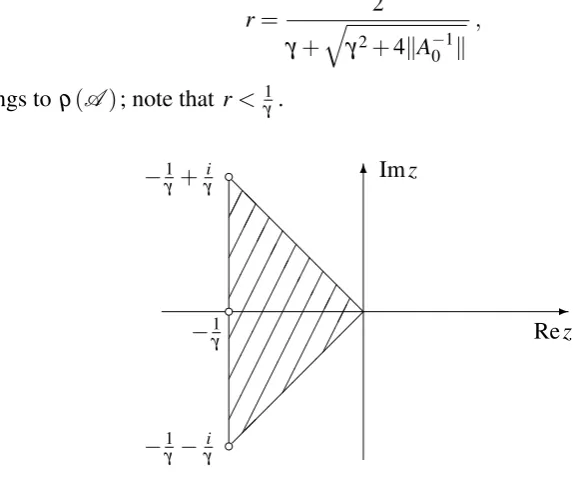
With the help of the form t(λ) it is shown in the following proposition that a
certain triangle belongs to the resolvent set of A ; see Figure 1. This complements [14,
Theorem 3.2], where it was shown that the open disc around zero with radius
r= 2
γ+ q
γ2+4kA−1 0 k
,
belongs to ρ(A); note that r< 1γ .
-6 @ @ @ @ @ @ b b b Rez Imz
−1γ −1γ +γi
[image:27.595.110.397.325.564.2]−1γ −γi
Figure 1: The region on the left-hand side of (4.19), which is contained in ρ(A); the
three circles indicate the numbers −1γ , −1γ ±γi, which, in general, do not belong to ρ(A).
PROPOSITION4.10. Assume that d6=0. Then
z∈C
z=0 or −1γ ≤Rez<0,argz∈ 3π
4 , 5π
4
/
−1γ ,−1γ ±γi
⊂ρ(A)
(4.19)
Proof. Since d6=0, we have D6=0 and γ>0, see (3.16). Letλ be either in the set on the left-hand side of (4.19) or let λ =−1γ and assume that γ 6=γ0 in the latter case.
Suppose that λ ∈σ(A). By Proposition 3.5 the set on the left-hand side of (4.19) is
disjoint from σess(A), and −1γ ∈/σess(A) if γ 6=γ0. Hence λ is an eigenvalue of A . By (4.7) there exists an x∈H1
2\ {0} such that t(λ)[x] =0. We have Re(λ)≥ −
1
γ and
Re(λ2)≥0, where at least one of the two inequalities is strict. Using (4.1) we therefore
obtain
0=Re t(λ)[x]=Re(λ2)kxk2+ (Reλ)d[x] +a0[x]
≥Re(λ2)kxk2+ (Reλ)γa0[x] +a0[x] >−1γ ·γa0[x] +a0[x] =0,
which is a contradiction. Hence λ ∈ρ(A).
One can easily construct examples with eigenvalues λ of A satisfying argλ ∈ π
2,34π
and |Reλ|< 1γ . For example, let A0 be a positive definite operator with compact resolvent and smallest eigenvalue 1/2. For the choiceD=A0, we have γ =1 and λ0=−14+i√47 is an eigenvalue of A which satisfies Reλ0=−1/4>−1γ =−1
and argλ0∈ π2,34π.
Another application of Theorem 4.8 results in interlacing properties of eigenvalues of two different second-order problems with coefficients that satisfy a specific order relation. This is the content of the following theorem.
THEOREM4.11. Let the forms a0, aˆ0, d anddˆ in the Hilbert space H be given
so that a0, d and aˆ0, dˆ, respectively, satisfy assumptions (F1)–(F3). Assume that
D(a0) =D(aˆ0) and
a0[x]≥aˆ0[x], d[x]≤dˆ[x] for x∈D(a0). (4.20)
Let Aˆ, δˆ, γˆ, δˆ0, γˆ0, ˆt, pˆ±, and αˆ be defined as in (3.10)–(3.11), (3.16), (3.17), (3.18), (4.3), and (4.9)–(4.11), respectively, where a0 is replaced by aˆ0 and d by d.ˆ
Then we have
γ ≤γˆ, γ0≤γˆ0, δ ≤δˆ, δ0≤δˆ0. (4.21)
Let
∆:= (a,0] with a≥max{α,αˆ}.
Assume now that σ(A)∩∆ is non-empty; then also σ(Aˆ)∩∆ is non-empty. Let (λn)Nn=1 and (λˆn)Nnˆ=1, N,Nˆ ∈N∪ {∞}, be the eigenvalues of A and Aˆ, respectively,
in the interval ∆, both arranged in non-increasing order and counted according their multiplicities. Then N≤N andˆ
Proof. The inequalities in (4.21) follow from (4.20), (3.20), (3.21), (3.22) and (3.17), e.g.
γ = sup y∈H1/2\{0}
d[y]
a0[y] ≤y∈Hsup1/2\{0}
ˆ
d[y]
ˆ
a0[y] =γˆ. The relations in (4.20) imply that
t(λ)[x]≥ˆt(λ)[x], x∈H1
2, λ ∈(−∞,0].
It follows from (2.4) that p+(x)≤pˆ+(x) for x∈H1
2 \ {0} and hence
µn:= sup L⊂H1/2
dimL=n
min
x∈L\{0} p+(x)≤L⊂supH1/2 dimL=n
min
x∈L\{0} pˆ+(x) =: ˆµn. (4.23) Assume that A has at least m eigenvalues in ∆. Then, by Theorem 4.8, λm=µm > a. If ˆA had less than m−1 eigenvalues in ∆, then ˆµm ≤a by (4.15), which is a
contradiction to (4.23). Hence the implication σ(A)∩∆6= /0 ⇒ σ(Aˆ)∩∆6= /0 and
the inequality N≤Nˆ are true. Finally, the inequality in (4.22) follows from (4.14) and (4.23).
5. Example: beam with damping
We consider a beam of length 1 and study transverse vibrations only. Let u(r,t)
denote the deflection of the beam from its rigid body motion at time t and position
r. We consider for the beam deflection a damping model which leads to the following description of the vibrations where a0 >0 is a real constant and d ∈C1[0,1] with minr∈[0,1]d(r)>0:
∂2u ∂t2 +a0
∂4u ∂r4 +
∂2 ∂t∂r
d∂u
∂r
=0, r∈(0,1),t>0. (5.1) Assuming that the beam is pinned, free to rotate and does not experience any torque at both ends, we have for all t>0 the following boundary conditions
ur
=0=u
r
=1=
∂2u ∂r2
r=0= ∂
2u ∂r2
r=1=0. (5.2)
We consider the partial differential equation (5.1)–(5.2) as a second-order problem in the Hilbert space H=L2(0,1). In order to formulate this beam equation as in (3.1), we
introduce the forms a0 andd defined for x,y from the form domains D(a0) =D(d) =
H2(0,1)∩H1
0(0,1) as
a0[x,y]:=a0 Z 1
0 x
00(r)y00(r)dr and d[x,y]:=Z 1 0 d(r)x
0(r)y0(r)dr. Then (5.1)–(5.2) corresponds to
Set
dmin:= min
r∈[0,1]d(r), dmax:=rmax∈[0,1]d(r).
For x∈D(a0) we have
a0[x] =a0hx00,x00i ≥a0π4kxk2,
which shows(F1). Using again kx00k ≥π2kxk we obtain for x∈D(a 0) that
a0[x] =a0kx00k2≥a0π2kx00kkxk ≥a0π2
Z 1
0 x
00(r)x(r)dr
=a0π2
Z 1
0
x0(r)2dr≥ a0π2
dmax Z 1
0 d(r)
x0(r)2dr= a0π2
dmaxd[x].
Thus(F2)holds. In order to show(F3)we introduce the operator A0 associated with
a0 via the the First Representation Theorem [15, Theorem VI.2.1] as in (3.2). It is easy to see that A0 has the form
A0=a0 d 4
dr4, D(A0) =
z
∈D(a0)|z00∈D(a0) .
Obviously, A0 satisfies assumption(F3). We define the Hilbert space H1
2 as in (3.3);
then H1
2 =D(a0) =D(d). Moreover, we define the damping operator as D:=−ddr
d d
dr
.
Due to the fact that d∈C1[0,1], D is a linear bounded operator from H1
2 to H. For x∈H1
2 we have
hDx,xi=hdx0,x0i=d[x].
Since DA−1/20 is a bounded operator in H and A−1/20 is a compact operator in H, we see that A−1/20 DA−1/20 is a compact operator in H. From this we obtain
σess A−1/20 DA−1/20 ={0}
and hence γ0=δ0=0. This, together with Proposition 3.5, yields
σess(A) = /0. (5.3)
Finally, we apply the results of this paper to the damped beam equation. THEOREM5.1. Assume that
Then D∗6= /0 (cf.(4.10)) and the number α from(4.11)satisfies α ≤ −dminπ22. The
set
σ(A)∩−dmin2π2,0
is non-empty and consists only of a finite sequence of isolated semi-simple eigenvalues of finite multiplicity ofA counted according to their multiplicities: λ1≥λ2≥. . .≥λN for some N∈N. The nth eigenvalue λn, 1≤n≤N , satisfies(4.14) in Theorem4.8 and the following inequalities:
λn≤
−dmax+
q
d2
max−4a0
2 ·π2n2, 1≤n≤N, (5.5)
and
λn≥− dmin+
q
d2
min−4a0
2 ·π2n2, n∈N such that n2≤
1 1−q1− 4a0
d2 min
. (5.6)
Note that the inequality in (5.6) for λn holds at least for n=1. Proof. We introduce the forms dmin and dmax by
dmin/max[x,y]:=dmin/max
Z 1
0 x
0(r)y0(r)dr, x,y∈H1
2,
the form polynomials tmin and tmax by
tmin/max(λ)[x,y]:=λ2hx,yi+λdmin/max[x,y] +a0[x,y], x,y∈H1 2,
and the corresponding operator functions Tmin and Tmax as in Proposition 4.3. Let
S:=−ddr22 in L2(0,1) with domain D(S) =H2(0,1)∩H01(0,1), which has spectrum σ(S) ={n2π2|n∈N}. Since we can write
Tmin/max(λ) =λ2+λdmin/maxS+a0S2,
we can use the spectral mapping theorem to obtain
σ(Tmin) =λ ∈C|λ2+λdminn2π2+a0n4π4=0 for some n∈N
= (
−dmin±
q
d2
min−4a0 2 ·n2π2
n∈N
)
⊂(−∞,0). (5.7)
In a similar way one obtains a description of σ(Tmax).
Define p±, p(±min), p(±max), D∗, Dmin∗ , Dmax∗ , α, αmin, αmax as in Definition 4.5
smallest eigenvalue, π2, of S with ke
1k=1, i.e. e1=√2sin(π·) and Se1=π2e1. It follows from (5.4) that
d[e1]−2ke1kpa0[e1]≥dmin[e1]−2pa0[e1]
=dminhSe1,e1i −2√a0kSe1k=dminπ2−2√a0π2≥0, which by (4.10) implies that D∗6= /0. Since γ0=0, we have
α = sup
x∈D∗p−(x) =xsup∈D∗
−d[x]− q
d[x]2−4kxk2a0[x] 2kxk2
≤ sup x∈D∗
−d[x]
2kxk2 ≤xsup ∈H1/2
−dmin[x]
2kxk2 =−x∈infH1
/2
dminkx0k2 2kxk2 =−
dminπ2 2 . In the same way one obtains that αmin,αmax≤ −dminπ
2
2 . Set ∆:= −dminπ2
2 ,0
and let (λn(min))Nn=min1 and (λn(max))Nmaxn=1 be the eigenvalues of Tmin and Tmax, respectively, in the interval ∆ ordered non-increasingly and counted with multiplicities. We can apply Theorem 4.11 to the pairs Tmin, T and T, Tmax, which implies that Nmin≤N≤Nmax and
λ(min)
n ≤λn, 1≤n≤Nmin,
λn≤λn(max), 1≤n≤N.
(5.8)
It follows from (5.7) that
λ(min)
n =−
dmin+
q
d2
min−4a0
2 ·n2π2, λ
(max)
n =
−dmax+
q
d2
max−4a0
2 ·n2π2. Moreover, Nmin is the largest positive integer such that
−dmin+
q
d2
min−4a0
2 ·Nmin2 π2≥ −
dminπ2 2 , where the latter inequality is equivalent to
Nmin2 ≤ dmin dmin−
q
d2
min−4a0
= 1
1−q1− 4a0 d2
min
. (5.9)
Now the inequalities in (5.8) imply (5.5) and (5.6). Since the right-hand side of (5.9) is greater than or equal to 1, we have N≥Nmin≥1. Hence σ(A)∩∆6= /0. Moreover,
N is finite because σess(A) =/0.
Acknowledgements