Lauren Marshall1,2 , Jill S. Johnson1 , Graham W. Mann1,3 , Lindsay Lee1 , Sandip S. Dhomse1 , Leighton Regayre1, Masaru Yoshioka1, Ken S. Carslaw1 , and Anja Schmidt4,5
1School of Earth and Environment, University of Leeds, Leeds, UK,2Now at Department of Chemistry, University of
Cambridge, Cambridge, UK,3National Centre for Atmospheric Science, University of Leeds, Leeds, UK,4Department
of Chemistry, University of Cambridge, Cambridge, UK,5Department of Geography, University of Cambridge, Cambridge, UK
Abstract
The radiative forcing caused by a volcanic eruption is dependent on several eruption source parameters such as the mass of sulfur dioxide (SO2) emitted, the eruption column height, and the eruption latitude. General circulation models with prognostic aerosol and chemistry schemes can be used to investigate how each parameter influences the volcanic forcing. However, the range of multidimensional parameter space that can be explored is restricted because such simulations are computationallyexpensive. Here we use statistical emulation to explore the radiative impact of eruptions over a wide covarying range of SO2emission magnitudes, injection heights, and eruption latitudes based on only 30 simulations. We use the emulators to build response surfaces to visualize and predict the sulfate aerosol
e-folding decay time, the stratospheric aerosol optical depth, and net radiative forcing of thousands of different eruptions. Wefind that the volcanic stratospheric aerosol optical depth and net radiative forcing are primarily determined by the mass of SO2emitted, but eruption latitude is the most important parameter in determining the sulfate aerosole-folding decay time. The response surfaces reveal joint effects of the eruption source parameters in influencing the net radiative forcing, such as a stronger influence of injection height for tropical eruptions than high-latitude eruptions. We also demonstrate how the emulated response surfaces can be used tofind all combinations of eruption source parameters that produce a particular volcanic response, often revealing multiple solutions.
1. Introduction
Volcanic eruptions emit SO2into the atmosphere, which is oxidized and forms sulfate aerosol. Sulfate aero-sol is very effective at scattering shortwave radiation, leading to surface cooling for a few years following a large-magnitude stratospheric volcanic eruption (e.g., Robock, 2000). The climatic effect of an eruption depends on several eruption source parameters, such as the mass of SO2emitted, the height of the SO2 emissions and the latitude of the volcano (e.g., Robock, 2000; Timmreck, 2012), as well as the season of eruption (e.g., Toohey et al., 2011) and the phase of the Quasi Biennial Oscillation (QBO; e.g., Thomas et al., 2009). It is important to understand the potential climatic impact of an eruption to evaluate the effects of historical eruptions and to assess the possible effects of future eruptions.
Several modeling studies have investigated the influence of important eruption source parameters but for only a limited number of eruptions (e.g., Dhomse et al., 2014; English et al., 2013; Jones et al., 2017; Metzner et al., 2014; Niemeier et al., 2009; Timmreck et al., 2010; Toohey et al., 2011, 2013). These studies also focus on the effects of variations in individual parameter values, which leaves almost all of the multi-dimensional parameter space unexplored. This modeling approach therefore creates a major problem for model interpretation if the parameter variations have nonlinear effects or if combinations of parameter per-turbations have effects that cannot be predicted from the combined effects of individual parameters.
The effects of eruptions vary a lot across the range of possible source parameters. Studies investigating the influence of SO2emission magnitude have shown that the climatic impact becomes self-limiting as the mass of emitted SO2increases (e.g., English et al., 2013; Metzner et al., 2014; Pinto et al., 1989; Timmreck et al., 2009) due to the formation of larger sulfate aerosol particles, which have a smaller optical depth per unit mass than smaller particles and are quickly deposited to the surface (Pinto et al., 1989). Furthermore, in eruptions with large SO2emissions, hydroxyl radicals (OH) in the ambient atmosphere, needed to oxidize
Special Section:
Stratospheric aerosol during the post Pinatubo era: processes, interactions, and impact
Key Points:
• We demonstrate the feasibility and value of using statistical emulation to quantify the radiative impact of volcanic eruptions
• Emulated response surfaces illustrate the dependencies of model output such as net radiative forcing on eruption source parameters • Emulated response surfaces can also
be used to constrain the eruption source parameters for a particular volcanic response
Supporting Information: •Supporting Information S1
Correspondence to: L. Marshall, [email protected]
Citation:
Marshall, L., Johnson, J. S., Mann, G. W., Lee, L., Dhomse, S. S., Regayre, L., et al. (2019). Exploring how eruption source parameters affect volcanic radiative forcing using statistical emulation.
Journal of Geophysical Research: Atmospheres,124, 964–985. https://doi. org/10.1029/2018JD028675
Received 16 MAR 2018 Accepted 8 DEC 2018
Accepted article online 17 DEC 2018 Published online 18 JAN 2019
©2018. The Authors.
the SO2, can become depleted (Bekki, 1995; Pinto et al., 1989). Eruptions in which the SO2is emitted higher into the stratosphere can have a greater climatic impact due to the residence time of stratospheric air increas-ing with distance from the tropopause and global transport if emitted at the equator (e.g., Robock, 2000). For stratosphere-injecting eruptions at high latitudes, aerosols are confined within the hemisphere and depos-ited to the surface more quickly (e.g., Kravitz & Robock, 2011; Oman et al., 2005, 2006). The effect of each of these parameters could be more or less important depending on the value of the other parameters, and a comprehensive and systematic investigation of such joint effects, while accounting for changes to the aero-sol particle size distribution, has not been conducted.
In this study, we use the approach of“designed experiments”(Sacks et al., 1989) and model emulation (O’Hagan, 2006) to efficiently map out how the outputs of an interactive stratospheric aerosol model (the U.K. Met Office Unified Model coupled with the U.K. Chemistry and Aerosol scheme [UM-UKCA]) vary across a three-dimensional parameter space. We do this by building surrogate statistical models (emulators) of several global model outputs (described in section 2) based on a set of simula-tions of erupsimula-tions with different SO2 emission magnitude, injection height, and latitude. We do not investigate the influence of eruption season or QBO phase. The emulator maps the relationship between the model output (such as radiative forcing) and the eruption source input parameters within an uncer-tainty (compared to the original model) that can be quantified. The emulator is very fast to evaluate and can be used to determine the impact of eruptions with parameter combinations that we did not expli-citly simulate, in a matter of seconds. As such, we can analyze model output without further runs of the computationally expensive model. We analyze how diagnostics describing the atmospheric impact of an eruption (section 2.4) vary with different SO2emission magnitudes, injection heights, and latitudes, and we are able, for thefirst time, to determine the effect of individual and combined parameter perturba-tions on the volcanic radiative forcing.
Section 2 describes the methods used in this study, including the experimental design of the UM-UKCA model simulations and details of the statistical emulation. In section 3.1 we show results from the simula-tions and in section 3.2 we present the results from the statistical emulators. We demonstrate the value of the emulators in section 3.3 by investigating the atmospheric impact of the 1991 eruption of Mount Pinatubo given a range in the estimated mass of SO2emitted and the injection height of the emissions. We also demonstrate how the emulators can be used tofind combinations of eruption source parameters for any given value of the model output. A summary and conclusions are found in section 4.
2. Methods
2.1. Model Description
We use the interactive stratospheric aerosol model UM-UKCA, which consists of the U.K. Met Office Unified Model (UM) general circulation model coupled with the U.K. Chemistry and Aerosol scheme (UKCA). In this study UM-UKCA is based on the“Global Atmosphere 4”(GA4) configuration of the UM (Walters et al., 2014) but includes the GLOMAP-mode aerosol microphysics scheme (Bellouin et al., 2013; Mann et al., 2010), which simulates aerosol mass and number concentrations using seven log-normal modes and UKCA whole-atmosphere chemistry, which combines the previous stratospheric (Morgenstern et al., 2009) and tropospheric (O’Connor et al., 2014) chemistry schemes. The model has a horizontal resolution of 1.875° by 1.25° with 85 vertical levels up to 85 km, resulting in well-resolved dynamics in the stratosphere and an internally generated QBO (e.g., Osprey et al., 2013). We performed atmosphere-only free running simulations with prescribed climatological sea surface temperatures and sea ice extent repeating at year 2000 conditions (Reynolds et al., 2007). Concentrations of greenhouse gases and ozone-depleting substances were also set at year 2000 levels.
The model setup is based upon the UM-UKCA version described in Dhomse et al. (2014), which includes stratospheric-tropospheric aerosol and interactive sulfur chemistry (including interactive OH chemistry), and simulated well the variations in stratospheric aerosol properties prior to and following the 1991 eruption of Mount Pinatubo compared to observations. The model treats the full lifecycle of stratospheric aerosol particles from initial injection of sulfur containing species, formation of gas-phase sulfuric acid following oxidation principally by OH, initial particle formation via binary homogeneous nucleation (Vehkamaki et al., 2002), and subsequent growth via condensation and coagulation.
Aerosol particles are removed from the stratosphere by sedimentation and dynamical exchange of air to the troposphere, where they are eventually deposited by wet and dry deposition. For the model simula-tions here, aerosol radiative heating is included (Mann et al., 2015) and the interactive stratospheric aerosol capability has been further improved (Brooke et al., 2017) to allow sulfuric particles to form het-erogeneously on transported meteoric smoke particle cores (MSP). The same model setup has also been applied in preindustrial condi-tions for the UM-UKCA 1815 Mount Tambora simulacondi-tions in Zanchettin et al. (2016) and Marshall et al. (2018).
In the chemistry scheme aerosol surface area is prescribed for the year 2000 (Thomason et al., 2008) and therefore the simulations do not account for the acceleration of heterogeneous chemistry on volcanically enhanced aerosol and subsequent radiative effects from changes to stratospheric ozone. However, the chemi-cal indirect effects from the eruptions arising from radiative dynamichemi-cally induced changes in stratospheric ozone, water vapor, and changes in heterogeneous chemistry from modified polar stratospheric clouds are resolved.
2.2. Choice of Eruption Source Parameters and their Values
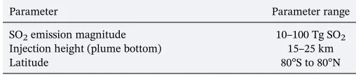
We investigate the effects of three key eruption source parameters: SO2 emission magnitude, injection height, and latitude, which are known to influence the climatic impact of a volcanic eruption (section 1). We choose to only perturb these three parameters for simplicity so that we can assess the feasibility of using statistical emulation in studies of volcanic forcing. The range of values over which we perturb each eruption source parameter is listed in Table 1, and the rationales behind these ranges are described below.
The SO2emission magnitude range of 10 to 100 Tg is chosen to cover an order of magnitude in eruption emission strength. This range also spans the estimated emissions from large-magnitude historical volcanic eruptions, often used as test cases to investigate the climatic effects of large sulfur injections, such as the 1991 eruption of Mount Pinatubo (~10–20 Tg SO2; Timmreck et al., 2018, and references therein) and the 1815 eruption of Mount Tambora (~60 Tg SO2; Zanchettin et al., 2016, and references therein). We vary the injection height over the range 15–25 km, with an injection depth of 3 km (i.e., injections from 15–18 to 25–28 km), so most of the SO2will be injected into the stratosphere. Our latitude range is near global to assess the full range of possible eruptions, omitting only the very highest latitudes at the edges of the model domain.
2.3. Simulation Design
The eruptions were simulated using parameter combinations (i.e., SO2 emission, injection height, and latitude) selected using the space-filling
[image:3.612.34.288.125.180.2]“maximin”Latin hypercube design algorithm (Morris & Mitchell, 1995) resulting in excellent coverage of the three-dimensional parameter space (Figure 1). The maximin algorithm maximizes the minimum dis-tance between all pairs of points in three-dimensional space so that each simulation is as far away as possible in parameter space from other simulations, while for each individual parameter we obtain a uniform coverage of the parameter range. Selecting the parameter com-binations of the simulations in this way provides maximum informa-tion for the emulator to capture variainforma-tions in the model responses across the whole parameter space. Based on previous model emulation studies (Johnson et al., 2015; Lee et al., 2011) and following the recom-mendation of Loeppky et al. (2009), we used 10 simulations per para-meter in the design, resulting in a total of 30 simulations to Table 1
Eruption Source Parameters and Range in Values That are Perturbed in This Study
Parameter Parameter range
SO2emission magnitude 10–100 Tg SO2
Injection height (plume bottom) 15–25 km
Latitude 80°S to 80°N
Figure 1.Volcanic eruptions simulated. Each triangle represents a model
simulation that was conducted. The location of the triangle indicates the latitude and injection height of the SO2emission for each eruption. The
injection height indicates the bottom of the emitted plume; emissions are distributed linearly between this value and 3 km higher, which is shown by the dots above each triangle. The size of the triangle represents the mass of SO2emitted. The simulations span SO2emissions between 10 and 100 Tg,
latitudes between 80°S and 80°N, and injection heights with a column bottom between 15 and 25 km. Red triangles are training runs, which are the simulations used to build the statistical emulators. Black triangles are simulations that were used to validate the statistical emulators after they were built. There are two simulations (one training run and one validation run) at ~63°S and ~17 km, which have SO2emissions of 35 and 45 Tg and
[image:3.612.40.284.447.581.2]construct our emulators. We refer to these simulations as “training runs”. We also ran a further 11 simulations that are used to validate the emulator once built, referred to as“validation runs”. The gen-erated simulations here do not necessarily represent the conditions of real volcanic eruptions (i.e., the latitude parameter values do not correspond to real volcano locations), but once we have built our emu-lators, we can predict the atmospheric responses for any volcanic eruption with parameter values within our perturbed parameter ranges. Additionally, the emulators we generate are also applicable to sulfur geoengineering studies where SO2 could be injected anywhere into the atmosphere (see section 2.5 for further details on the emulation itself).
Figure 1 shows our simulation design with each triangle representing a model simulation. All eruptions are 24 hr in duration and are simulated on 1 July, during the easterly QBO phase, and at 160°E longitude where many real volcanoes do exist, and eruptions are frequent (Global Volcanism Program, 2013). The longitude of an eruption is not important for determining the climatic impact (e.g., Toohey et al., 2011) since aerosol in the stratosphere is rapidly transported around the globe, but our simulations have the added benefit of cover-ing realistic eruption locations. Each simulation was run for 38 months followcover-ing the eruption, and we ana-lyze monthly mean model output. We also run a control simulation with no eruption to diagnose the volcanic anomalies.
2.4. Model Outputs
We focus on three key model outputs that determine the magnitude and duration of the volcanic forcing: (1) the global volcanic sulfate burdene-folding decay time (in months), (2) the time-integrated global mean vol-canic stratospheric aerosol optical depth (sAOD) at 550 nm (in months), and (3) the time-integrated global mean net radiative forcing (MJ/m2). The derivation of each output is outlined below.
The sulfatee-folding decay time is defined as the time it takes for the global volcanic sulfate burden (i.e., the sulfate mass anomaly compared to a quiescent background) to decay to 1/eof its peak value. This is a mea-sure of the sulfate aerosol lifetime, which will determine the longevity of the volcanic radiative forcing. Volcanic sulfate aerosol does not decay with a constante-folding timescale (e.g., Stratosphere-troposphere Processes And their Role in Climate, 2006); therefore, we calculate an averagee-folding time from thefit of a linear regression line to the natural logarithm of the global sulfate burden anomalies (e.g., Pitari et al., 2016). Wefit the regression line from 1 month after the peak burden until the burden has decayed to below 10% of the peak burden. This calculation method accounts for different durations of the atmospheric volcanic perturbations between the different eruptions. We refer to this as the“average global sulfatee-folding decay time”, and an example of the derivation is included in the appendix.
Integrated global mean sAOD is the sum of the monthly mean anomalies in global mean sAOD at 550 nm following each eruption, which is influenced by the number and size of sulfate aerosol particles. Integrated global mean net radiative forcing is the sum of the top-of-the-atmosphere outgoing global mean all-sky net radiativeflux anomalies (shortwave [SW] + longwave [LW]). The anomalies are inte-grated over 38 months (until the end of the simulation). For all eruptions the anomalies have decayed to below 10% of the peak anomaly by the end of the simulation.
2.5. Emulation and Sensitivity Analysis
For each model output we construct a Gaussian process emulator that maps how the output depends on the input parameters over the three-dimensional parameter space. The emulator is a surrogate statistical representation of the UM-UKCA model. It is built by assuming that the model response is a Gaussian process and updating the parameters of this Gaussian process with the training data (Kennedy & O’Hagan, 2001; O’Hagan, 2006). An overview of this statistical methodology is given in Appendix A of Johnson et al. (2015) and Lee et al. (2011). The emulator is fast to evaluate and can be used to pre-dict the output quantity at any combination of the input parameters, enabling multidimensional response surfaces of output behavior across parameter space to be generated.
Emulators have been used in several studies to analyze complex models in multiple scientificfields including tsunami modeling (Sarri et al., 2012), aerosol and cloud modeling (e.g., Carslaw et al., 2013; Hamilton et al., 2014; Johnson et al., 2015; Lee et al., 2013; Regayre et al., 2014, 2015), and galaxy formation (Rodrigues et al., 2017; Vernon et al., 2010). A recent study by Harvey et al. (2018) also successfully applied this approach to
volcanic ash modeling of the 2010 Eyjafjallajökull eruption to understand the influence of eruption source parameters and internal model parameters on the simulated output.
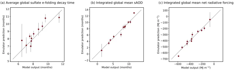
Each emulator is constructed from the output of the training runs using the statistical software R (R Core Team, 2017) and the DiceKriging package (Roustant et al., 2012). We build separate emulators for the average global sulfatee-folding decay time, the integrated global mean sAOD, and the integrated global mean net radiative forcing (section 2.4). The emulators are built assuming a linear mean function that includes all parameters and a Matérn covariance structure, which allows for slight variations in smoothness in the output response (Rasmussen & Williams, 2006). Further details regarding fitting the emulators using these assumptions can be found in Johnson et al. (2015). To validate the emulators, we use them to predict the model values at the parameter setting of each validation run and compare the prediction to the actual model output of these runs (Figure 2). For the integrated global mean sAOD, the model output lies within the 95% confidence bounds of the emulator prediction for the majority of the validation runs. For the integrated global mean net radiative forcing the emulator also performs well but is overly confident, with the emulator predictions having small confidence bounds that do not always cross the 1:1 line marking a perfect emulator prediction. We only take forward the emulator mean prediction for our analysis, which lies very close to the 1:1 line in all cases, so for our purposes it does not matter that the emulator is too confident at times. Additionally, with small emulator errors, we are confident that emulator error does not have any significant effect on the pre-sented analysis and results. The average global sulfatee-folding decay time emulator validates less well. There is more variability on how closely the emulator can predict model output in this case, with three validation points that are overestimated by the emulator, and for which the model output lies outside the 95% confidence bound of the emulator prediction. This emulator is less confident in its predictions overall (the 95% confidence bounds are larger). However, the e-folding timescale evolves differently throughout the decay period for each of our simulated eruptions (very few of our eruptions simulated exhibit perfect exponential decay of the global sulfate aerosol burden). Hence, the tightness of thefit of the regression line to the sulfate burden decay time series varies between simulated eruptions. Because this model output cannot perfectly describe the sulfate decay behavior of all eruptions simu-lated, we expect greater uncertainty in the emulator representation for this output and conclude that this emulatorfit is not unreasonable.
[image:5.612.175.576.90.209.2]Using the validated emulators, we sample each output quantity at thousands of parameter combinations of the SO2emission magnitude, injection height, and latitude that we did not explicitly simulate with UM-UKCA. By densely sampling the emulators across the parameter space defined by the ranges in Table 1, we can map response surfaces that show how each output responds to changes in the input parameters. We can also use statistical techniques such as variance-based sensitivity analysis (Saltelli et al., 2000) to quantify the sensitivity of each output to variation in individual parameters. This is achieved by implementing the extended Fourier Amplitude Sensitivity Test approach of Saltelli et al. (1999) to decompose the total variance in the output quantity over the parameter space into individual and joint parameter contributions (section 3.2.3) using the R package“sensitivity” (Pujol et al., 2017).
Figure 2.Validation of each emulator. For each model output (a–c), the value of the model output for the 11 validation
runs is plotted against that predicted by the emulator (red circles). The vertical lines are 95% confidence bounds on the emulator predictions. The solid gray line marks the 1:1 line, indicating a perfect prediction by the emulator.
3. Results and Discussion
3.1. Model Output Over the Set of Eruption Simulations
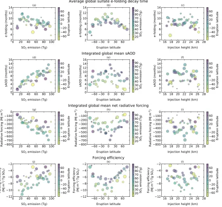
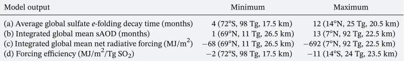
Before emulating, wefirst examine the model output across the 41 simulations. Figure 3 shows the average global sulfatee-folding decay time (a–c), the integrated global mean sAOD anomalies (d–f), and the inte-grated global mean net radiative forcing (g–i). In addition, we also show the net radiative forcing efficiency calculated as the integrated net forcing divided by the mass of SO2emitted (MJ/m2/Tg SO2; j–l). Each of these output quantities is shown for each simulation plotted against the eruption source parameters.
3.1.1. Sulfate Burdene-Folding Decay Time
[image:6.612.83.540.95.520.2]Figures 3a–3c show that the average global sulfate e-folding decay time is dependent on latitude with longer e-folding decay times for eruptions at low latitudes resulting from slower removal of the
Figure 3.Model outputs versus the eruption source parameters for all 41 model simulations (training and validation). Each plotted point represents the output of
one model simulation. For each output quantity (each row), we show the output value versus SO2emission (a, d, g, and j), eruption latitude (b, e, h, and k; negative values indicate the southern hemisphere), and injection height (c, f, i, and l). For plots in the leftmost column the color of the points indicates the latitude of the eruption in each simulation and the size indicates the injection height (the larger the point, the higher the injection height). For the plots in the middle column, the color represents the mass of SO2emitted and the size indicates the injection height. In the right column, the color indicates the latitude of the eruption and the
size represents the mass of SO2emitted (the larger the point, the larger the SO2emission). The injection height values are the center of each 3-km plume. sAOD = stratospheric aerosol optical depth.
aerosol and shortere-folding decay times for eruptions at high latitudes resulting from faster removal of the aerosol. These differences are due principally to the stratospheric Brewer-Dobson circulation (BDC), which is characterized by upward motion at the tropics, poleward transport, and downward motion at the poles (e.g., Butchart, 2014; Holton et al., 1995). The global sulfate e-folding decay times also decrease with increasing SO2 emission magnitudes because of growth to larger particle sizes and increased gravitational sedimentation. The e-folding decay time generally increases as the injection height increases until the height of the SO2 emission is ~21 km, although the response is weaker compared to that of the eruption latitude and SO2 emission (Figures 3a and 3b). The increase in decay time with injection height is a result of longer air residence time. However, for injection heights greater than ~21 km thee-folding decay time starts to decrease. The decrease in the average decay time (i.e., shorter aerosol lifetime) above ~21 km is contrary to the general increase in air residence time with height because it is complicated by aerosol microphysical processes (i.e., aerosol growth) and latitude-dependent circulation features and meridional transport barriers, such as the tropical pipe (Plumb, 1996). The average decay time reflects several phases of the aerosol evolution. For example, longer-lived volcanic sulfate aerosol particles have more time to grow by condensation and coagulation and therefore sediment more rapidly later during the aerosol decay, such that the average e-folding time decreases. We find that the ratio of the integrated global mean sAOD at 550 nm to the sAOD at 1,020 nm, which is a proxy of particle size, decreases with increasing injection height, indicating that larger particles are formed on average for eruptions with higher-altitude injections (not shown). Sedimentation rates are also higher with increasing higher-altitude since the air density is reduced. The influence of stratospheric dynamics and aerosol microphysics is explored in greater detail in section 3.2.2.
By examining the colors of the points in Figure 3a, we can begin to see joint dependencies between the SO2 emission magnitude and latitude in influencing thee-folding time: for low-latitude eruptions (blue points) the reduction in thee-folding time with increasing SO2emission appears stronger than for high-latitude eruptions (yellow and purple points) where the points are more variable. Overall, the average sulfate aerosol
e-folding decay time is strongly variable, ranging from 4 to 12 months (Table 2).
3.1.2. Integrated Global Mean sAOD and Net Radiative Forcing
Integrated global mean sAOD (Figures 3d–3f) ranges from 1 to 13 months (Table 2) and has a strong dependency on the mass of SO2emitted with higher integrated sAOD for greater SO2emissions. This is due primarily to the formation of more sulfate aerosol mass. Integrated global mean sAOD is also greater for lower-latitude eruptions and for eruptions with the altitude of the SO2emission near 22 km, likely refl ect-ing the increase in aerosol lifetime and a decrease in scatterect-ing efficiency for higher-altitude injections following the formation of larger particles. As with the sulfatee-folding decay time (Figures 3a–3c), there is greater variation in the integrated sAOD versus the injection height.
Integrated global mean net radiative forcing (Figures 3g–3i) is also stronger for larger SO2emissions, low-latitude eruptions, and injection heights around ~22 km. The integrated net radiative forcing ranges from
[image:7.612.173.576.116.177.2]68 to692 MJ/m2. Like the sulfatee-folding decay time, we can also begin to see some joint dependencies between the amount of SO2emitted and latitude in the increase in net radiative forcing. Net radiative forcing strengthens more rapidly (becomes more negative) with increasing SO2emission for low-latitude eruptions (blue points) compared to high-latitude eruptions (yellow and purple points). Dependencies are explored in greater detail using the statistical emulators (section 3.2).
Table 2
Model Outputs Considered and Summary Statistics Across the 41 Eruptions Simulated
Model output Minimum Maximum
(a) Average global sulfatee-folding decay time (months) 4 (72°S, 98 Tg, 17.5 km) 12 (14°N, 25 Tg, 20.5 km) (b) Integrated global mean sAOD (months) 1 (69°N, 11 Tg, 26.5 km) 13 (7°N, 92 Tg, 22.5 km) (c) Integrated global mean net radiative forcing (MJ/m2) 68 (69°N, 11 Tg, 26.5 km) 692 (7°N, 92 Tg, 22.5 km) (d) Forcing efficiency (MJ/m2/Tg SO2) 2 (72°S, 98 Tg, 17.5 km) 11 (14°S, 24 Tg, 23.5 km)
The increase in net radiative forcing is not linear with increasing SO2emission. Figures 3j–3l show that the forcing efficiency weakens with increasing SO2emissions, in line with previous modeling studies of volcanic eruptions and sulfate geoengineering studies (e.g., English et al., 2013; Kleinschmitt et al., 2018; Niemeier & Timmreck, 2015; Timmreck et al., 2010). The weakening in forcing efficiency is predominantly due to a decrease in the SW efficiency as aerosol particles increase in size and become less effective at scattering SW radiation. The LW forcing efficiency is more constant for increasing SO2emission (Figure S1 in the sup-porting information). As a result, the net radiative forcing efficiency decreases (the forcing becomes less negative). The net forcing efficiency is higher for low-latitude eruptions because of an increase in the SW effi -ciency, but the LW efficiency also increases for low-latitude eruptions, which offsets some of the forcing by SW radiation. This increased forcing efficiency is due to increased insolation and outgoing radiation and likely the longer aerosol lifetime at low latitudes. Against injection height, the forcing efficiency is greatest for eruptions with emission altitudes near 22 km. The most effective eruption (per teragram of SO2mass emitted) occurs at a latitude of 14°S with 24 Tg SO2emitted between 22 and 25 km. The least effective erup-tion is at 72°S, with 98 Tg SO2emitted between 16 and 19 km (Table 2).
3.2. Multidimensional Analysis Using Statistical Emulation 3.2.1. Emulated Response Surfaces
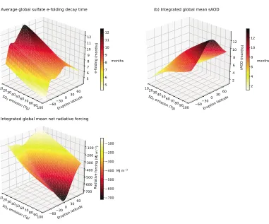
[image:8.612.192.573.83.400.2]We use the validated emulators (Figure 2) for each model output to predict the output at other parameter combinations that we have not explicitly simulated. Figure 4 shows example response surfaces that reveal the relationship between each model output and the value of latitude and the mass of SO2emitted, at a fixed injection height of 20–23 km. For visualization purposes, injection height wasfixed at its central
Figure 4.Emulated response surfaces for each model output (a–c) at afixed injection height of 20–23 km. The surface
shows the emulator’s prediction of the model response (zaxis) against the mass of SO2emitted (xaxis) and latitude (y axes). The color of the surface also indicates the value of the predicted model output. Each surface is plotted from 1,600 combinations of latitude and SO2magnitude, which were determined over a grid of 40 equally spaced values of each varied parameter between the minimum and maximum parameter input values (Table 1). sAOD = stratospheric aerosol optical depth.
value in the emulator as this parameter has the weakest relationship with each of the model outputs (Figure 3).
The surfaces in Figure 4 further demonstrate the dependencies of the model outputs on the mass of SO2 emitted by an eruption and its latitude. The average global sulfatee-folding decay time shows a stronger dependence on the value of latitude, with a sharp gradient observed in the response surface across the lati-tude dimension. Thee-folding decay time is more than 12 months for eruptions at the equator that have less than ~24 Tg of SO2emitted. The surfaces for integrated global mean sAOD and integrated global mean net radiative forcing are more similar, with strong gradients across the SO2emission magnitude dimension espe-cially for low-latitude eruptions.
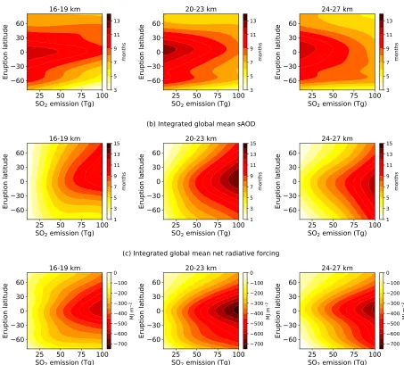
[image:9.612.77.530.102.511.2]To explore the relationship between the model outputs and the latitude and SO2emission of an eruption for other injection heights, we also sample the emulated response surface atfixed injection heights of 16–19, 20– 23, and 24–27 km and show these surfaces in two dimensions (Figure 5).
Figure 5.Emulated response surfaces atfixed injection heights for each model output. For each emulator (a–c), we sample atfixed injection heights of 16–19, 20–23
(as in Figure 4), and 24–27 km. The resulting contour plots show the emulator prediction of each model output against SO2emission and latitude of the eruption at
Now we begin to see more clearly the influence of injection height on each model output because the response surfaces are not the same at each height. For example, for injections at 20–23 km, all model outputs reach greater values. The symmetry across latitude also changes with height; for example, at 16–19 km, inte-grated sAOD for SO2emissions greater than ~50 Tg is larger for eruptions in the Northern Hemisphere (NH) than in the Southern Hemisphere (SH). However, the surface is more symmetrical across latitude for injec-tions at 20–23 and 24–27 km.
[image:10.612.72.531.96.517.2]Figure 6 shows the emulated response surfaces plotted against the SO2 emission and injection height (center of the plume) atfixed latitudes of 60°S, 0°, and 60°N. At 60°S the integrated sAOD and radiative forcing are highest for eruptions that have injection heights above ~22 km and the highest emissions. However, for emissions less than ~50 Tg, the highest forcing occurs for eruptions with emission alti-tudes nearer 21 km. For eruptions at the equator, the largest integrated sAOD and radiative forcing occur for injection heights near 22 km for all SO2emissions. At 60°N, the model outputs are less sen-sitive to injection height than for eruptions at 60°S and 0° and are mainly dependent on the SO2
Figure 6.Emulated response surfaces atfixed latitude for each model output. For each emulator (a–c), we sample atfixed latitudes of 60°S, 0°, and 60°N. The
result-ing contour plots show the emulator prediction of each model output against SO2emission and the middle injection height of the emissions (i.e., center of the 3-km
plume) at each of these latitudes. sAOD = stratospheric aerosol optical depth.
emission. For the sulfate e-folding decay time, the surfaces are more variable, and since this emulator validated the least well, we focus on the general patterns only. In general, the decay time decreases for larger SO2 emissions and at 0° decreases for the high-altitude injections of low SO2emissions.
Figure 7 shows the response surfaces at fixed SO2 emissions of 20, 45, and 80 Tg. Here we see the dependency that the model outputs have on latitude and injection height at these emission magnitudes. In general, these surfaces are more similar in shape, with peaks in each model output for eruptions at the equator and for injection heights at ~22 km. At higher latitudes, the model outputs are less depen-dent on the value of injection height. The surfaces are also not entirely symmetrical around the equator.
The surfaces also reveal that the same model outputs can be achieved for notably different combinations of parameter values. For example, the more circular contours in Figure 7b for an injection of 45 Tg (middle panel) show that an integrated sAOD of 6–7 months can be caused by an eruption at 0° with the SO2injected at 26 km or an eruption at 60°S with the SO2 injected at 20 km.
3.2.2. Mechanisms for the Parameter Dependencies
[image:11.612.86.518.97.493.2]Figures 5–7 consolidate the patterns and responses revealed by the individual simulations (Figure 3) but allow us to explore the relationships at any point in parameter space, in which the dependencies of the
Figure 7.Emulated response surfaces atfixed SO2emissions for each model output. For each emulator (a–c), we sample atfixed SO2emissions of 20, 45, and 80 Tg.
output on the eruption source parameters change. Thee-folding decay time of the sulfate aerosol is a function of the large-scale stratospheric BDC and sulfate particle sizes, which dictates the sedimentation rate. The integrated sAOD is a function of the mass of sulfate aerosol, its size distribution, and the sulfatee-folding decay time. The integrated net radiative forcing is dependent on the volcanic sAOD and additionally the inso-lation, cloud cover, and surface albedo. In general, the varying responses in Figures 5–7 can be explained by differences in the large-scale stratospheric circulation and in aerosol microphysical processes and are explored below.
3.2.2.1. Tropical Eruptions
For tropical eruptions, the model outputs were more dependent on injection height than for eruptions in the high latitudes, with a turning point at roughly 22 km for the integrated global mean sAOD and net radiative forcing (e.g., Figure 7). In the tropics, sulfate aerosol transport is influenced by the stratospheric tropical pipe (Plumb, 1996), which extends from roughly 21 to 28 km and restricts meridional transport from the tropics to the extratropics (Trepte & Hitchman, 1992). Consequently, sulfate aerosol builds up in the tropical reservoir after an eruption. However, in the lower stratosphere the rapid shallow branch of the BDC allows greater transport of the aerosol to high latitudes, and with increasing altitude, the strength of the tropical barrier reduces (e.g., Holton et al., 1995), and smaller aerosol particles, which have not sedimented out, can be trans-ported to the extratropics in the upper branch of the BDC (e.g., Niemeier & Schmidt, 2017). Arfeuille et al. (2014) found that sulfate aerosol simulated after the 1815 eruption of Mount Tambora had a shorter resi-dence time in the tropics and stronger extratropical transport for a 27- to 29-km injection compared to a 23- to 25-km injection, which is comparable to the results presented here.
In addition to variations in the strength of subtropical transport barriers, the response to injection height in the tropics is also in part due to changes in sulfate aerosol particle size and sedimentation. The time-integrated and global nature of these outputs means that several phases of the aerosol evolution are averaged and reflected in just one number. We suggest that in general there are two phases of the aerosol evolution. Thefirst phase is a“growth phase”as the aerosol particles form and coagulate, in which aerosol removal mainly depends on the latitude of the eruption rather than the SO2emission. The second“sedimentation phase”occurs after several months when particle growth has slowed and sedimentation becomes relatively more important. We suggest that longer air residence time and subsequent growth to larger particles for SO2injections above ~22 km increases the sedimentation rate and hence aerosol decay in the second phase of the aerosol evolution, causing a decrease in the integrated global mean sAOD and net radiative forcing. Radiative forcing is also weakened because larger particles are less effective at scattering SW radiation. Similar effects are also observed in geoengineering simulations of continuous sulfur emissions with increas-ing injection heights, such that the effects of a longer lifetime and larger particles cancel, and radiative forcincreas-ing does not increase with higher-altitude SO2injections (e.g., Kleinschmitt et al., 2018; Niemeier & Schmidt, 2017; Tilmes et al., 2017).
As the mass of SO2emitted is increased from 20 to 45 Tg, the maximum values of the average global sulfate
e-folding decay time, integrated sAOD, and radiative forcing occur at decreasing injection heights (Figure 7), likely related to increased sedimentation as particles grow larger for the bigger SO2emissions. This is also seen in the average global sulfatee-folding decay time as the emission is increased from 45 to 80 Tg, but this is not the case for the integrated sAOD and radiative forcing. The peak value in the average sulfatee-folding decay time also occurs for lower injection heights compared to the peak values in integrated sAOD and radiative forcing. The sulfatee-folding decay time reflects the loss of sulfate aerosol mass, but the sAOD is dependent on the aerosol surface area. As the particles grow and sediment, which decreases the average aerosol lifetime, the remaining smaller particles are more optically efficient; hence, the integrated sAOD remains higher. Increased upwelling due to aerosol-induced radiative heating may increase the tropical
con-finement and aerosol lifetime (e.g., Niemeier et al., 2009, 2011) when the strongest volcanic forcing occurs, despite a lower averagee-folding decay time, which reflects all phases of the aerosol decay. For the higher-altitude injections, enhanced lofting may also result in the aerosol moving to higher-altitudes at which the tropical barrier is weaker, allowing it to spread meridionally (e.g., Aquila et al., 2012; Young et al., 1994). Additionally, higher temperatures at high altitudes may reduce the amount of gaseous sulfuric acid that nucleates, and some of the formed aerosol may then evaporate, reducing the sulfate aerosol mass. Some of this vapor can also condense onto MSP, where it remains (in this version of UM-UKCA), and photolysis of sulfuric acid vapor will also produce SO2. However, wefind that the proportion of global sulfur that is
in the form of gaseous sulfuric acid compared to sulfate aerosol is very small in all of the 41 simulations. The largest fraction of global sulfur accommodated onto MSP compared to the total sulfate aerosol plus gaseous sulfuric acid at any time in a simulation was 0.23. These effects are unlikely to significantly contribute to the response to injection height shown here.
Aerosol radiative heating can also modify the QBO (e.g., Aquila et al., 2012, 2014; Kleinschmitt et al., 2018; Niemeier & Schmidt, 2017), which further modulates the tropical confinement and transport of sulfate aerosols out of the tropics (e.g., Punge et al., 2009; Trepte & Hitchman, 1992; Trepte et al., 1993). Although beyond the scope of the present study, such dynamical changes induced by the sulfate aerosol are likely contributing to the response in the model output as the SO2emission increases.
3.2.2.2. Mid- to High-Latitude Eruptions
Outside of the tropical pipe, the lifetime of sulfate aerosol is dependent on the large-scale meridional trans-port, isentropic mixing, and transport to the troposphere via midlatitude tropopause folds, sedimentation, and large-scale subsidence, where it is eventually deposited by wet and dry deposition (e.g., Hamill et al., 1997). For mid- to high-latitude eruptions, the effect of injection height on the model outputs is less pro-nounced than those at low latitudes, as aerosol is not restricted by the tropical pipe, and due to the much faster decay times of sulfate aerosol there is less time for the growth of particles to offset an otherwise increase in aerosol lifetime with increasing altitude.
Eruptions with middle injection heights (~19–23 km) in the SH have larger values of the model outputs than the equivalent eruptions in the NH (e.g., Figures 5 and 7), although this is not the case for all emission magnitudes and latitudes. Because our eruptions occurred in July, large-scale mixing, poleward transport, and deposition are stronger in the winter SH at the time of the eruption (Holton et al., 1995). Insolation at the time of the eruption is greater in the NH, but in the majority of our simulations, the peak aerosol burden occurs ~5–6 months after the eruption, consequently coinciding with the peak summer insolation if the eruption was in the SH and resulting in a larger radiative forcing. Climatologically, transport is stronger in the NH and therefore over the integrated time period NH erup-tions may have a lesser impact as more of the aerosol plume is transported into the troposphere. Differences in the global model output between eruptions in each hemisphere are also related to the surface albedo and other aspects of the stratospheric dynamics such as the position of the tropopause and the polar winter vortices. The tropopause is lower in the SH (Figure 1) such that the lowest injec-tions in the NH will be closer to the tropopause where the aerosol is removed more effectively via isen-tropic transport and tropopause folds compared to the equivalent SH eruption. The polar winter vortices at ~60° inhibit transport of aerosol to the poles, but effectively remove aerosol that is within the vortex, and the vortex is stronger in the SH (Hamill et al., 1997; Holton et al., 1995).
The rate of the initial SO2oxidation may also contribute to some of the differences in the surfaces, although the effect is difficult to disentangle from the mechanisms discussed above. For example, wefind that the
e-folding decay time of the SO2increases the larger the SO2emission (i.e., slower oxidation) due to OH depletion, is longer for high-latitude eruptions because of lower OH concentrations, and is slightly shorter following eruptions in the summer hemisphere (Figure S2). Slower SO2oxidation can lead to a prolonged radiative forcing because particles do not grow as large and are longer-lived and more effective at scattering radiation (e.g., Bekki et al., 1996). We do notfind a significant difference in the SO2e-folding decay time for tropical eruptions with different injection heights but a greater variation in the decay time for high-latitude eruptions (Figure S2).
3.2.3. Average Response of the Model Output
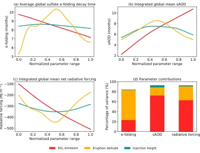
Figure 8 shows the average response of each model output to each eruption source parameter over the three-dimensional parameter space (a–c) and the percentage contribution that each parameter makes to the model output value (d), calculated from a variance-based sensitivity analysis (section 2.5). Figures 8a–8c are partial dependence plots that integrate over all other dimensions except the one that is varied. Emulation prediction uncertainty is also accounted for by averaging over random draws of the emulator response surfaces from thefitted Gaussian process uncertainty. The sensitivity analysis allows quantification of the features and trends seen in the initial scatter plots and response surfaces (Figures 3–7).
The red lines in Figure 8 show the response to SO2emission from low to high emissions, which results in a decrease in aerosol decay time, and an increase in integrated global mean sAOD and net radiative forcing. The response to injection height (teal) from low to high altitudes is seen most clearly for the integrated sAOD. The response to latitude (orange) from high southern latitudes to high northern latitudes is most dominant for the sulfatee-folding decay time. Interestingly, the average response shows a ridge in the response to latitude in the mid- to high-latitudes in the SH, which is apparent for the sulfatee-folding decay time and net radiative forcing but not for sAOD. The exact cause of the decrease in response remains uncer-tain but could be influenced by increased stratosphere-troposphere exchange in the jet stream regions and deposition of aerosol in the SH storm tracks for the sulfatee-folding decay time and due to the seasonally varying insolation for the radiative forcing.
[image:14.612.181.574.89.391.2]For all three model outputs, the injection height is relatively the least important parameter, contributing to less than 5% of the variance in each output. As a result, any change in the model outputs by changing the
Figure 8.Sensitivity analysis results showing the average effects of the SO2emission magnitude (red), eruption latitude
(orange), and injection height (teal) on the value of each model output (a–c) and the percentage of variance in each model output explained by each eruption source parameter (d). The average responses are plotted against the normalized parameter range showing the effects from low to high SO2emissions (10 to 100 Tg), from high SH latitudes to high NH
latitudes (80°S to 80°N) and from low injection heights to high injection heights (bottom of the plume from 15 to 25 km). sAOD = stratospheric aerosol optical depth.
injection height is dwarfed by changes to the SO2emission magnitude and latitude. For the average global sulfatee-folding decay time, the SO2 emis-sion explains 23% of the variance and latitude explains 60%. However, for the integrated global mean sAOD, we see the opposite situation, where the SO2emission contributes more to the variance at 72% compared to 16% from the latitude. The integrated global mean net radiative forcing is sensitive to the parameters in a very similar way as we see for the inte-grated global mean sAOD but with a slightly lower contribution from the SO2emission (63%) and a slightly higher contribution from latitude (28%). The contributions suggest that the decay rate of the sulfate aerosol is pri-marily dependent on the stratospheric circulation, but the integrated sAOD and radiative forcing depend primarily on the SO2emission, which dictates the amount of aerosol that can form. The slightly larger contribu-tion from latitude for integrated radiative forcing compared to the inte-grated sAOD is likely due to the fact that although primarily a function of the sAOD, the radiative forcing is also dependent on the insolation, cloud cover and surface albedo, which vary as a function of latitude. The variance contributions do not total to 100% as the total variance is also explained by possible interaction effects (the combined effect of each para-meter with the other parapara-meters) and random noise. In general, this con-tribution is very small and likely noise related.
In the following section we explore some of the novel applications of the emulated surfaces.
3.3. Emulator Applications
3.3.1. Emulator Predictions for the 1991 Eruption of Mount Pinatubo
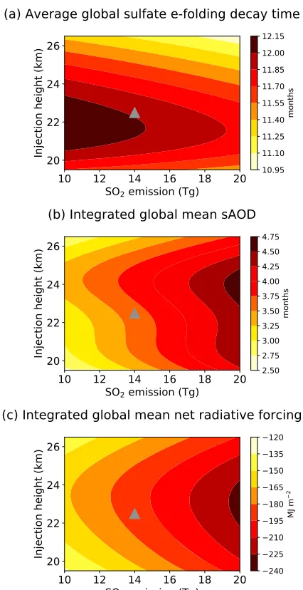
The emulators can be used to predict the atmospheric effects of historic eruptions that have eruption source parameters within our simulated ranges. There is substantial uncertainty in both the mass of SO2emitted and the injection height of emissions for historic eruptions due to a lack of direct observations and to limitations in available observations. We can use the emulators to quantify the range of a model output that is con-sistent with the estimated uncertainty range of the eruption source para-meters. As an example, Figure 9 shows the emulator response surfaces for parameter ranges relevant to the 1991 eruption of Mount Pinatubo (latitude 15°N). For one possible realization of this eruption (the gray triangle), with 14 Tg of SO2emitted between 21 and 24 km, the emulator predicts an average global sulfatee-folding time of 12 months, integrated global mean sAOD of 3.6 months, and integrated global mean net radiative forcing of187 MJ/m2. When we account for the uncertainties in the erup-tion source parameters (SO2emissions of 10–20 Tg and injection heights spanning 18–25 km; Timmreck et al., 2018, and references therein), we predict an average global sulfatee-folding decay time of ~11–12 months, an integrated global mean sAOD of ~2.7–4.6 months, and integrated global mean net radiative forcing of about133 to229 MJ/m2.
[image:15.612.56.269.87.501.2]Our estimates of average global sulfatee-folding decay time, regardless of the combination of SO2 emis-sion and injection height, are in good agreement with observations and previous model simulations, which reporte-folding decay times of about 1 year (e.g., SPARC, 2006). The equivalent integrated global mean sAOD at 550 nm from the CMIP6 data set (version 3; Thomason et al., 2018) is ~2.5 months (we calculate post-Pinatubo sAOD anomalies by subtracting an estimate of the background sAOD using years 1999–2000) and is slightly less than the minimum value of ~2.7 months predicted by the emulator when emitting 10 Tg SO2 between 18 and 21 km.
Figure 9.Emulated response surfaces at the latitude of Mount Pinatubo for
each model output (a–c). These surfaces show the predicted model outputs for possible combinations of the SO2emission and injection height
esti-mated for the 1991 eruption of Mount Pinatubo. We sample a grid of 10,000 parameter combinations with the SO2emission ranging between 10 and
20 Tg (100 equally spaced values) and injection height between 18 and 25 km (100 equally spaced values representing the bottom of the plume) and lati-tudefixed at 15°N. The gray triangle marks one possible realization of the 1991 eruption with an SO2emission of 14 Tg and injection height of
We can also use the emulators“in reverse”tofind the ranges of the eruption source parameters that are con-sistent with a particular volcanic response. For example, as seen in Figure 9b, there are other parts of the parameter space that can result in an integrated global mean sAOD close to 2.7 months. Toohey et al. (2011) calculated a 4-year integrated global mean volcanic AOD after the eruption of Mount Pinatubo of ~3 months using a 17 Tg SO2 emission, which is comparable to our results. The light yellow region in Figure 9b shows the combinations of SO2emission and injection height that result in integrated sAOD less than 3 months. The SO2emissions must be less than ~12 Tg, but the injection height (center of the plume) can either be less than ~21 km or greater than ~26 km (given the assumed range in SO2emission and injec-tion height). Of course, not all combinainjec-tions of the constrained SO2emission and injection height will result in an integrated global mean sAOD less than 3; for example, if the mass of SO2emitted was 12 Tg, the injec-tion height could not be 21 km.
To match the integrated sAOD value of ~2.5 from CMIP6 for the 1991 Mount Pinatubo eruption, UM-UKCA requires SO2emissions nearer 10 Tg, with an injection height nearer 19.5 km (Figure 9b). The small mismatch between the CMIP6 value of integrated sAOD and the emulator prediction suggests that the CMIP6 value is too low, UM-UKCA has overestimated the atmospheric perturbation, or the true SO2 emission and injection height laid outside of our estimated ranges (10–20 Tg and 18–25 km). The UM-UKCA simulations were also idealized, with an assumed 3-km plume depth and were not nudged to 1991 meteorology, which has been shown to influence the initial plume dispersal (e.g., Jones et al., 2016). However, since the two estimates are very similar, and the estimated global sulfatee-folding decay time also agrees well with observations, the emulators do a very good job at capturing the effects of the 1991 Mount Pinatubo eruption, reflecting the validity of the emulators and the idealized UM-UKCA simulations.
[image:16.612.95.518.90.337.2]Constraint of the eruption source parameters using the emulators is not limited to historic eruptions. They can be used to constrain the eruption source parameter combinations for any given value or range of values of the model outputs across the full three-dimensional parameter space (section 3.3.2).
Figure 10.Parts of parameter space that result in an integrated global mean stratospheric aerosol optical depth (sAOD) greater than 10 months. (a–c) Histograms of
the individual constrained parameter values using 10 bins. The dashed gray lines mark the median values. (d–f) The combinations of two parameters that remain after constraint. The color indicates the density of parameter combinations (lighter = fewer points; darker = more points). Panels (d) to (f) are annotated in regions of the parameter space where the integrated global mean sAOD is not greater than 10 with explanations of why the sAOD values are lower. Injection height is the center of the 3-km plume.
3.3.2. Parameter Combinations That Result in Integrated sAOD>10
We further demonstrate the value of the emulators by identifying parts of the eruption source parameter space that result in an integrated global mean sAOD greater than 10 months. An integrated value of 10 is roughly 3 times greater than that from the 1991 eruption of Mount Pinatubo. We take a uniformly gridded sample of one million combinations covering the full three-dimensional parameter space (using 100 equally spaced values across each of the parameter ranges in Table 1) and evaluate the sAOD output at each combi-nation using the emulator. We then retain only the parameter combicombi-nations that match our criterion of sAOD>10. These resulting parameter combinations are plotted in Figure 10. The top row displays histo-grams of each individual constrained parameter, and the bottom row shows the two-dimensional projections of the parameter space that remains on constraint. The color indicates the density of parameter combina-tions in that part of remaining parameter space. A three-dimensional view can be obtained using the online tool.
Only eruptions in which more than ~56 Tg of SO2is emitted have the potential to produce an integrated glo-bal mean sAOD of at least 10 (Figures 10a, 10d, and 10f) as sufficient sulfate aerosol must be formed. This is approximately the magnitude of the mass of SO2 emitted during the 1815 eruption of Mount Tambora (Zanchettin et al., 2016). However, the injection height is not constrained and the middle of the plume can be at any height between 16.5 and 26.5 km (i.e., with a column bottom between 15 and 25 km) (Figures 10c–10e). The volcano must be situated between ~80°S and ~67°N (Figures 10b, 10e, and 10f), with higher-latitude NH eruptions leading to too rapid decay of the sulfate aerosol burden to sustain an sAOD
>10. The constrained space in Figure 10 enables the joint three-dimensional parameter space to be explored. For example, for emission magnitudes in the lower part of the range, the injection height must be nearer the middle of the range and the eruption must be near the equator. The eruption can only result in an integrated global mean sAOD>10 with an injection height of 26 km (center of the 3-km plume) if the SO2emission is greater than ~79 Tg. In general, as the SO2emissions increase and as the eruption moves toward lower lati-tudes an integrated sAOD>10 becomes more likely (i.e., there are more values of injection height that can be combined with these other two parameters to produce sAOD>10). At the extremes of the injection height integrated sAOD>10 is less likely. Figure 10 also reveals some interesting shapes in the surfaces. For exam-ple, Figure 10e is asymmetrical around the equator and the eruption can occur at higher southern latitudes with high injection heights than in the NH. This is likely a seasonal response, given that our eruptions occur in July but may also reflect differences in circulation strength and patterns between the two hemispheres, such as the polar winter vortex.
4. Summary and Conclusions
We have investigated the influence of the mass of SO2emitted (between 10 and 100 Tg), eruption latitude (between 80°S and 80°N), and injection height of the emissions (between 15 and 25 km with an injection depth of 3 km) on the radiative forcing of a large-magnitude explosive eruption, using a state-of-the-art general circulation model with interactive aerosol microphysics. We have focused on three model outputs to understand the radiative impact: the global sulfatee-folding decay time, the time-integrated global mean sAOD, and the time-integrated global mean net radiative forcing. In contrast to conventional climate model experimental designs in which parameters are perturbed in isolation, we simulated 41 eruptions each with different combinations of the three eruption source parameter values. Using Gaussian process emulators, we then predicted model output for parameter combinations that we did not explicitly simulate. We calculated the average response of each model output to each parameter and quantified the relative importance of each parameter.
SO2emitted and eruption latitude, the injection height is in relative terms the least important parameter, contributing to less than 5% of the variance in each model output. Any change to the net radiative forcing by changing the injection height is dwarfed by any changes to the SO2emission magnitude and eruption lati-tude. Efforts to diagnose the global and time-integrated climatic impact of eruptions should therefore focus on determining the initial mass of SO2released rather than the injection altitude.
We have demonstrated that statistical emulation is a suitable and powerful tool for investigating the volcanic radiative forcing of past and future eruptions. First, despite only running 41 model simulations, the emu-lated response surfaces allow us to predict in a matter of seconds the global sulfatee-folding decay time, the time-integrated global mean sAOD, and the time-integrated net radiative forcing of any eruption in the latitude range 80°S to 80°N, SO2emission between 10 and 100 Tg, and emission injection height (column bottom of 3-km-thick plume) between 15 and 25 km (e.g., Figures 5–8). An online tool has been provided in which two-dimensional and three-dimensional emulated response surfaces for all combinations of eruption source parameters can be explored and constrained.
Second, the emulated surfaces expose relationships between the parameters and the model output across the whole parameter space, which in a conventional experimental design would have been difficult to see. For example, wefind that the dependency of the net radiative forcing on injection height is more important for tropical eruptions than for eruptions in the high latitudes (e.g., Figure 7). The emulated surfaces have revealed many compensating effects between stratospheric circulation, sedimentation, and the scattering efficiency of particles in determining the net radiative forcing, which were not obvious from analyzing the model output alone (Figure 3).
Third, the emulators allow us to quantify the relationships between each parameter and the model output such that we can determine the relative importance of each and calculate the average effect of each para-meter on the model output across the whole parapara-meter space (Figure 8).
Finally, we have also shown that the emulators can be used to constrain the eruption source parameters for a given volcanic response (Figure 10), revealing multiple solutions.
The emulators are not limited to the three-dimensional space presented here nor to the three model outputs that we chose. For example, we have built 27-dimensional emulators to understand aerosol effective radia-tive forcing (Regayre et al., 2018), 11-dimensional emulators to understand deep convecradia-tive cloud behavior (Johnson et al., 2015), and attempted to observationally constrain 28-dimensional emulators of tropospheric aerosol processes (Lee et al., 2016). In relation to volcano-climate studies, future work could explore the con-tributions of other eruption source parameters such as plume depth, eruption duration, season of eruption, and QBO phase. These additional parameters could influence the importance of the three parameters pre-sented here. However, the emulated surfaces still provide afirst-order estimate of the effects of each of these parameters, which are still likely to be the most important. Our simulations also started with the same meteorological conditions, and variations in meteorology could alter the initial plume evolution (e.g., Jones et al., 2016). However, since the stratospheric dynamics can be modified by aerosol radiative heating and the fact that we have analyzed global and time-integrated output, the effect of initial conditions is likely second order to that of the eruption source parameters. In simulations of the 1815 Mount Tambora eruption we also found little variation among ensemble members with different initial conditions (Marshall et al., 2018). Other model outputs such as peak responses or regional impacts, which are likely to have larger extremes, could also be explored using this novel methodology.
Our results have highlighted the importance of aerosol microphysical processes such as sedimentation in determining the magnitude of the volcanic forcing, but model parameterizations of aerosol microphysical processes in volcanic clouds such as nucleation and sedimentation are also important causes of model uncer-tainties (e.g., English et al., 2013). Changes to particle coagulation schemes, for example, with the inclusion of Van der Waals forces, have been shown to change aerosol distributions (e.g., English et al., 2013; Sukhodolov et al., 2018). Future ensembles in which the model process parameters are perturbed would allow quantification of the sensitivity of volcanic forcing to the model’s aerosol microphysics (e.g., Johnson et al., 2015; Lee et al., 2013; Regayre et al., 2018). Future sensitivity studies in which sedimentation is switched off completely and simulations with the same SO2emission injected at various points in the tro-pical pipe would aid in investigating some of the nonlinearities discovered in this study.
Appendix A.: Derivation of the Average Global Sulfate
e
-Folding Decay Time
To determine the average global sulfatee-folding decay time, we plot the natural logarithm of the monthly mean global sulfate burden anomalies from the peak burden andfit a linear regression line from 1 month after the peak burden to until the burden has fallen below 10% of the peak burden (Figure A1). Fitting from one month after the peak ensures that the sulfate burden is decaying; however, the timing of the main phase of decay does differ between eruptions.We calculate the averagee-folding decay time by taking thefitted sulfate burden from thefirst and last values of the regression line:
efolding time¼ðt2t1Þ=log b1
b2
whereb1 is the burden calculated from thefirst value of the regression line andb2 is the burden calculated from the last value of the line (b=eburden). Thet2t1 equals the time in months between the two burdens.
References
Aquila, V., Garfinkel, C. I., Newman, P. A., Oman, L. D., & Waugh, D. W. (2014). Modifications of the quasi-biennial oscillation by a geoengineering perturbation of the stratospheric aerosol layer.Geophysical Research Letters,41, 1738–1744. https://doi.org/10.1002/ 2013GL058818
Aquila, V., Oman, L. D., Stolarski, R. S., Colarco, P. R., & Newman, P. A. (2012). Dispersion of the volcanic sulfate cloud from a Mount Pinatubo-like eruption.Journal of Geophysical Research,117, D06216. https://doi.org/10.1029/2011JD016968
Arfeuille, F., Weisenstein, D., Mack, H., Rozanov, E., Peter, T., & Bronnimann, S. (2014). Volcanic forcing for climate modeling: A new microphysics-based data set covering years 1600-present.Climate of the Past,10(1), 359–375. https://doi.org/10.5194/cp-10-359-2014
Bekki, S. (1995). Oxidation of volcanic SO2: A sink for stratospheric OH and H2O.Geophysical Research Letters,22(8), 913–916. https://doi. org/10.1029/95GL00534
Bekki, S., Pyle, J. A., Zhong, W., Toumi, R., Haigh, J. D., & Pyle, D. M. (1996). The role of microphysical and chemical processes in prolonging the climate forcing of the Toba Eruption.Geophysical Research Letters,23(19), 2669–2672.
Bellouin, N., Mann, G. W., Woodhouse, M. T., Johnson, C., Carslaw, K. S., & Dalvi, M. (2013). Impact of the modal aerosol scheme GLOMAP-mode on aerosol forcing in the Hadley Centre Global Environmental Model.Atmospheric Chemistry and Physics,13(6), 3027–3044. https://doi.org/10.5194/acp-13-3027-2013
Brooke, J. S. A., Feng, W. H., Carrillo-Sanchez, J. D., Mann, G. W., James, A. D., Bardeen, C. G., & Plane, J. M. C. (2017). Meteoric smoke deposition in the polar regions: A comparison of measurements with global atmospheric models.Journal of Geophysical Research: Atmospheres,122, 11,112–11,130. https://doi.org/10.1002/2017JD027143
[image:19.612.258.487.306.474.2]Butchart, N. (2014). The Brewer-Dobson circulation.Reviews of Geophysics,52, 157–184. https://doi.org/10.1002/2013RG000448
Figure A1.Global volcanic sulfate burden (log(e)Tg S) for one example model simulation (red line and scatter points)
from the maximum monthly mean burden and linear regression line (dashed line)fitted from 1 month after the peak burden up until the burden falls below 10% of the peak burden. The averagee-folding decay time is calculated using the fitted regression line.
Acknowledgments
L. M. was funded by the U.K. Natural Environment Research Council (NERC) through the Leeds-York NERC Doctoral Training Program (NE/ L002574/1). A. S., K. S. C., and G. W. M. received funding from NERC grant NE/ N006038/1 (SMURPHS). J. S. J. and K. S. C. acknowledge funding from NERC grant NE/J024252/1 (GASSP). L. R. and K. S. C. acknowledge funding from NERC grant NE/P013406/1 (A-CURE). J. S. J. and K. S. C. were supported by the U.K.-China Research and Innovation Partnership Fund through the Met Office Climate Science for Service Partnership (CSSP) China as part of the Newton Fund. G. W. M. received funding from the National Centre for Atmospheric Science (NCAS), one of the NERC research centers via the ACSIS long-term science program on the Atlantic climate system. M. Y. acknowledges funding from NCAS. K. S. C. is currently a Royal Society Wolfson Merit Award holder. We are extremely grateful to Richard Rigby (University of Leeds, now at the British Antarctic Survey) for providing the online tool, the link to which is included in the supporting information. The authors also thank Grenville Lister for facilitating the running of this ensemble, Andy Jones and Jim Haywood for useful discussions, and Editor Zhanqing Li, the Associate Editor, and three anonymous reviewers for their helpful and constructive reviews that greatly improved this manuscript. This work used the ARCHER UK National
Supercomputing Service (http://www. archer.ac.uk) and JASMIN super-data-cluster (doi:10.1109/