This is a repository copy of
The optimal kinematic dynamo driven by steady flows in a
sphere
.
White Rose Research Online URL for this paper:
http://eprints.whiterose.ac.uk/126104/
Version: Accepted Version
Article:
Chen, L, Herreman, W, Li, K et al. (3 more authors) (2018) The optimal kinematic dynamo
driven by steady flows in a sphere. Journal of Fluid Mechanics, 839. pp. 1-32. ISSN
0022-1120
https://doi.org/10.1017/jfm.2017.924
© 2018, Cambridge University Press. This article has been published in a revised form in
Journal of Fluid Mechanics https://doi.org/10.1017/jfm.2017.924. This version is free to
view and download for private research and study only. Not for re-distribution, re-sale or
use in derivative works. Uploaded in accordance with the publisher's self-archiving policy.
[email protected] https://eprints.whiterose.ac.uk/ Reuse
Items deposited in White Rose Research Online are protected by copyright, with all rights reserved unless indicated otherwise. They may be downloaded and/or printed for private study, or other acts as permitted by national copyright laws. The publisher or other rights holders may allow further reproduction and re-use of the full text version. This is indicated by the licence information on the White Rose Research Online record for the item.
Takedown
If you consider content in White Rose Research Online to be in breach of UK law, please notify us by
The optimal kinematic dynamo driven by
steady flows in a sphere
L. Chen
1, W. Herreman
2, K. Li
1, P. W. Livermore
3, J. W. Luo
1and A. Jackson
1†
1Institute of Geophysics, ETH Zurich, Sonneggstrasse 5, Zurich, 8092, Switzerland
2
LIMSI, CNRS, Universit´e Paris-Sud, Orsay, 91405, France
3
School of Earth and Environment, University of Leeds, Leeds, LS2 9JT, United Kingdom
(Received ?; revised ?; accepted ?. - To be entered by editorial office)
We present a variational optimisation method that can identify the most efficient kine-matic dynamo in a sphere, where efficiency is based on the value of a magnetic Reynolds number that uses enstrophy to characterize the inductive effects of the fluid flow. In this large scale optimisation, we restrict the flow to be steady and incompressible, and the boundary of the sphere to be no-slip and electrically insulating. We impose these bound-ary conditions using a Galerkin method in terms of specifically designed vector field bases. We solve iteratively for the flow field and the accompanying magnetic eigenfunction in order to find the minimal critical magnetic Reynolds numberRmc,min for the onset of
a dynamo. Although nonlinear, this iteration procedure converges to a single solution and there is no evidence that this is not a global optimum. We findRmc,min= 64.45 is
at least three times lower than that of any published example of a spherical kinematic dynamo generated by steady flows, and our optimal dynamo clearly operates above the theoretical lower bounds for dynamo action. The corresponding optimal flow has a spa-tially localized helical structure in the centre of the sphere, and the dominant components are invariant under rotation byπ.
Key words:variational methods, dynamo theory
1. Introduction
The Earth, as well as certain other planets, moons and stars, is known to possess a self-sustaining magnetic field. Such magnetic fields are generated via fluid motion in a confined conductive interior through a process that is termed dynamo action (Moffatt 1983). Mathematically such dynamics can be modelled by a coupled system of differential equations referred to as magnetohydrodynamics (MHD). If we prescribe the flow fieldU
and ignore the backreaction from the magnetic fieldBonU, we obtain a simple system called the kinematic dynamo problem. In this reduced system, one can study how a flow field amplifies a seed magnetic field. Early numericists found flow fields that are capable of dynamo action in a sphere with electrically insulating boundary conditions (Backus 1958; Pekeriset al.1973; Kumar & Roberts 1975; Gubbins 1973; Dudley & James 1989). However, there is no universal recipe on how to obtain such flow fields; known dynamo solutions do not necessarily share similar spatial structures (Gubbins 2008).
Optimisation offers a tool to explore the many possible ways of getting dynamo ac-tion. Historically optimisation of dynamo models has taken place predominantly with
2 L. Chen, W. Herreman, K. Li, P. W. Livermore, J. W. Luo and A. Jackson
a restricted type of velocity field: for example, working in a sphere, Love & Gubbins (1996b) optimized the flow proposed by Kumar & Roberts (1975) (abbreviated as KR) while Holme (2003) optimized flows proposed by Dudley & James (1989) (abbreviated as DJ); later studies by Love & Gubbins (1996a); Holme (1997); Gubbinset al.(2000a) and Gubbinset al. (2000b) yielded more efficient solutions using only poloidal flows of KR type. Allied work also includes the search for optimal dynamos driven by ABC flows in a periodic domain (Alexakis 2011), maximization of helicity for the cylindrical Riga experiment (Stefaniet al.1999), optimisation of boundary driven flows for the spherical Madison plasma experiment (Khalzov et al. 2012), optimisation of flow structures and conducting layers for the cylindrical VKS experiment (Marie et al.2003; Ravelet et al.
2005), and most recently, the study of optimal forcing for chaotic dynamos (Sadeket al.
2016). From a more fundamental point of view, we want to ask: “Imposing no constraints other than the spherical boundaries, what is the most efficient dynamo, and what are its characteristics?”. Optimisation that potentially covers an infinitely large parameter space of flow structures, is needed to answer these questions.
A variational approach has successfully optimized kinematic dynamo models in a cube (Willis 2012; Chen et al. 2015; Herreman 2016). This method sets up a Lagrangian consisting of an objective functional that usually measures the magnetic energy at later times, subject to a number of constraints, then searches for the optimal state, i.e. a stationary point of the Lagrangian in phase space with respect to the variation of each variable, including that of the velocity field and the seed magnetic field. The important control parameter in optimisation is the magnetic Reynolds numberRm. It measures the effects of advection and stretching of magnetic field compared to the effects of Ohmic decay. In order to sustain dynamo action,Rm must be sufficiently large such that field creation outweighs field destruction through dissipation, and indeed Rm must exceed certain known lower bounds (Backus 1958; Busse 1975; Childress 1969; Proctor 1977, 1979). Historically, different definitions of Rm have been used, and one needs to be careful which measure to use. It has been proven that the kinetic energy-based magnetic Reynolds number (denoted byRmu) has no lower bound (Proctor 2015), since a given
flow field can be shrunk to a smaller region with a lower value of Rmu while dynamo
action is retained through the increased shear. As a consequence we use an enstrophy-based normalization to defineRm in our optimisation which is equivalent to normalizing the global magnitude of shear.
In this work, we extend these previous studies to find the optimal kinematic dynamo in a sphere. As a first step, our aim is to look for optimal dynamo action among gen-eral steady and incompressible flows in a sphere with widely-used electrically insulating and no-slip boundary conditions. This requires the use of an inner product defined over infinite space, which we refer to as an all-space norm, and a primitive formulation of the Lagrangian. The all-space norm removes all surface integrals during the derivation of the variations of the Lagrangian and is key to the successful application of our method. We also developed an adjoint model for this particular optimisation problem, akin to those first written down by Namikawa & Matsushita (1970) and Liet al.(2011). Lastly, a specially constructed orthogonal Galerkin basis (Livermore & Ierley 2010; Livermore 2010; Li et al.2010) for the vector fields ensures a rapid convergence in spectral space towards the optimal state.
The structure of this article is as follows: we introduce the methodology in §2 and present the results in §3, wherein we describe the optimal flow field, together with its magnetic eigenvector at the minimal critical magnetic Reynolds number for the onset of dynamo actionRmc,min= 64.45. We discuss the characteristics of this optimal solution,
compare Rmc,min directly with the optimized dynamo models in a cube (Chen et al.
2015) by rescaling typical length scales and volumes in§3.8. We close with conclusions in§4.
2. Methods
2.1. Definition of the optimisation objective
Consider a sphere V∗ filled with an electrically conducting fluid. Outside the sphere,
we suppose a current free region ˆV∗ that extends to infinity. IfL∗ denotes dimensional
values for the spherical radius andη∗ denotes the fluid’s magnetic diffusivity, we then
non-dimensionalize the flow field using units [U] =ω∗L∗for velocity, [x] =L∗ for length
and [t] =L∗2/η∗ for time. Hereω∗ is the dimensional root mean enstrophy,
ω∗=
s
1
V∗
Z
V∗
(∇×U∗)2dV∗, (2.1)
V∗is the dimensional volume of the sphere, andU∗is the dimensional velocity field; we
setη∗= 1/(µ∗
0σ∗), whereµ∗0is permeability of free space,σ∗is the electrical conductivity. The magnetic Reynolds number is then defined as
Rm=ω
∗L∗2
η∗ . (2.2)
Note here it is necessary to use the enstrophy measure of flow strength for reasons explained in the introduction. In this model, we impose no-slip boundary conditions on the flow fieldU∗. This then leads to the condition that the root mean enstrophyω∗=S∗,
whereS∗=q 1
V∗
R
V∗2e ∗
ij e∗ij dV∗is the dimensional global shear magnitude, ande∗ij
is the dimensional strain rate tensor.
The non-dimensionalized flow fieldU =U(x) lives within the parameter space Eu of
all steady and incompressible fields with no-slip boundary conditions, i.e.∀U ∈ Eu,
∇·U = 0, x∈ V, (2.3)
U|Σ− =0, (2.4)
where we denote by Σ±either the outer surface (+) or the inner surface (−) of the sphere
at the interface between non-dimensionalized domainsV and ˆV. In a kinematic approach, the magnetic fieldB and the electric fieldE need to satisfy the non-dimensional equa-tions,
E=∇×B−Rm U×B, x∈ V, (2.5)
∂tB=−∇×E, x∈ V ∪Vˆ, (2.6)
∇×B=0, x∈Vˆ, (2.7)
∇·B= 0, x∈ V ∪Vˆ. (2.8)
We have used an arbitrary scale [B] to non-dimensionalize the magnetic field, and [E] =
ω∗L∗[B] to non-dimensionalize the electric field. Unlike in Willis (2012) and Chen et al.
4 L. Chen, W. Herreman, K. Li, P. W. Livermore, J. W. Luo and A. Jackson
condition, equation (2.8) is Gauss’ law for magnetism, and we also impose the continuity conditions,
B|Σ+−B|Σ− =0, ˆr× E|Σ+−E|Σ−
=0, (2.9)
where ˆris the radial unit vector. Since the flow is steady, the kinematic dynamo problem admits exponential solutions for the magnetic field,
B(x, t)∼b(x)e(γ+iΩ)t, (2.10) whereb(x) is an eigenvector,γ is the growth rate and Ω is an oscillation frequency. As
t→ ∞, one can expect that the eigenvector with the largest growth rate will eventually dominate the solution, assuming an arbitrary noisy initial magnetic fieldB0=B(x,0). In this optimisation study, we want to identify the flow field U ∈ Eu that maximizes
the growth rate γ for a given value of Rm, and subsequently find the lower bound on the critical magnetic Reynolds number, denoted byRmc,min, below which no kinematic
dynamo is possible∀U ∈ Eu.
2.2. Euler-Lagrange formalism in primitive format
Since we want to optimize the growth rateγ, it seems most obvious to propose an opti-misation method that directly maximizesγ. This can indeed be done in low-dimensional optimisation problems, see for example Holme (2003). However, considering the infinitely large dimension of the functional spaceEu we have, optimising the growth rate directly
is not practical. Instead, we adapt the optimisation strategy of Willis (2012); Chenet al.
(2015); Herreman (2016) that proved successful in a cube. These methods are designed to find the optimal flow field U and seed magnetic field B0 that maximize a specified global measure of BT, where BT = B(x, T) is the magnetic field at some finite time
T that needs to be long enough to overcome initial transient growth phases. Optimising
B0then allows us to reach this exponential regime faster. It is worth remarking that, in general, the initial fieldB0 that has greatest projection onto the most rapidly growing eigenvectorBT is the corresponding eigenvector of the related adjoint eigenvalue problem
(Farrell & Ioannou 1996) (distinct from the adjoint formalism we will use). However, we opt to discover the structure ofB0 directly by an optimising scheme as we will set out below, rather than introducing the additional complexity of solving the adjoint eigenvalue problem.
The variational method we use is built on the following Lagrangian:
L= ln(BT)2
−λ1
1
V
(∇×U)2−1
−λ2 (B0)2−1
− hΠ∇·Ui −
Z T
0
ψ†∇·B dt−
Z T
0
D
B†·[∂tB+∇×E]
E
dt
−
Z T
0
D
E†·[σrE+Rm U×B−∇×B]
E
dt. (2.11)
We denote the volume of domainV byV, the all-space integral:
h . . . i=
Z ∞
0
Z 2π
0
Z π
0 · · ·
at timeT. From the second to the last term in (2.11), we impose a series of constraints in this model, namely the normalization constraint forU andB0, the solenoidal conditions on U and B, Faraday’s law and Amp`ere’s law. Note that the flow field U is entirely confined to the sphere V, so there is no contribution to the enstrophy from ˆV. The variablesλ1, λ2, Π(x),ψ†(x, t), B†(
x, t) and E†(x, t) are Lagrange multipliers. Π, ψ†, B†,E† are often referred to subsequently as adjoint fields. The numberσr is a relative
electrical conductivity:
σr=
1, x∈ V,
0, x∈Vˆ. (2.13)
At the optimum the LagrangianL(U,B,B0,BT,E, λ1, λ2,Π, ψ†,B†,E†) must be sta-tionary, meaning that δL = 0 for arbitrary variations in each of its variables. Each variational derivative needs to disappear separately, which defines eleven Euler-Lagrange (EL) equations in our optimisation problem. The physical constraints define six equa-tions: the solenoidal conditions as in (2.3) and (2.8), the normalization constraints on
B0 andU, Amp`ere’s law and Faraday’s law. The remaining five non-trivial variational derivatives are
δL δBT
= 2BT
h(BT)2i−
B†T, (2.14)
δL
δE =−σrE †
−∇×B†, (2.15)
δL δB =∂tB
†+Rm
U×E†+∇×E†+∇ψ†, (2.16)
δL δU =Rm
Z T
0
B×(−σrE†) dt−2λ1∇×∇×U+∇Π, (2.17)
δL δB0
=B†0−2λ2B0, (2.18)
where B†T =B†(x, T) and B†0 =B†(x,0). A number of boundary terms arise during the derivation of these non-trivial variational derivatives by partial integration, and their sum needs to cancel at the optimum in order to have a consistent theory. In this model, the magnetic fieldB decays at least as fast asr−3 in the insulating region ˆV, whereris the distance to the origin, so all boundary variations on the surface of ˆV as r→ ∞are negligible. We then need all boundary terms to cancel on Σ±:
0 =−
I
Π(ˆr·δU)Σ
−dS−
I
2λ1
h
δU×(∇×U)i·ˆrΣ −dS
+
Z T
0
I h
(ˆr×B†)·δEΣ
−−(ˆr×B †)
·δEΣ
+
i
dS dt
+
Z T
0
I h
(ˆr×E†)·δBΣ
−−(ˆr×E †
)·δBΣ
+
i
dS dt
−
Z T
0
I h
ψ†(ˆr·δB)Σ
−−ψ †(ˆr
·δB)Σ
+
i
dS dt. (2.19)
If we suppose that the field variations δU satisfy no-slip conditions (2.4), the first two boundary terms are zero. Then, the inclusion of the external region ˆV allows us to cancel the remaining boundary terms by matching them from Σ− to Σ+. The primitive
formal-ism also allows us to simplify the treatment of boundary terms on Σ±: using continuity
6 L. Chen, W. Herreman, K. Li, P. W. Livermore, J. W. Luo and A. Jackson
(2.9), we immediately obtain the boundary conditions for the adjoint fields,
ψ†|
Σ+−ψ
†|
Σ− = 0, ˆr×(B †
|Σ+−B
†
|Σ−) = 0, ˆr×(E †
|Σ+−E
†
|Σ−) = 0. (2.20)
Because of (2.15) and the presence of ∇ψ† in (2.16), the adjoint magnetic field has
a gauge degree of freedom B† → B† +∇φ. Therefore, we can add a supplementary
requirement that the adjoint magnetic field is also solenoidal,
∇·B† = 0, x∈ V ∪Vˆ. (2.21)
along with the boundary condition, ˆ
r·(B†|Σ+−B
†
|Σ−) = 0. (2.22)
By requiring the sum of all boundary terms to vanish, we just derived the continuity conditions forψ†,B† and
E†. This brings us to the conclusion that, with a gauge degree of freedom, adjoint fields B† and E† satisfy exactly the same boundary conditions as the direct fieldsB andE. This is an eminently desirable property, since it allows us to use the same solenoidal Galerkin expansions for both direct fieldB and adjoint fieldB†
later in§2.4.
2.3. Reduced set of Euler-Lagrange equations
Now we have dealt with the boundary terms, we can eliminate the fieldsE andE†from the previous “primitive” set of EL equations and present the reduced set of EL equations that we will actually solve. We build an optimisation loop that will locate the stationary point of the Lagrangian (2.11) iteratively. Upon initialization (possibly combined with an update) and at each iteration in the optimisation loop, the flow fieldU and the seed magnetic fieldB0 satisfy the normalization constraints,
1
V
(∇×U)2= 1, (B0)2= 1, (2.23) the solenoidal conditions (2.3) and (2.8), and the boundary conditions (2.4) and (2.9).
In the optimisation loop itself, there are three parts: a forward integration, a backward integration and an update, similar to the procedure described by Kerswellet al.(2014). First we solve the forward/direct problem. In region ˆV, the magnetic field satisfies (2.7). In region V, by combining Amp`ere’s law and Faraday’s law, we solve the induction equation forward in time fort: 0→T,
∂tB=Rm∇×(U×B)−∇×(∇×B), x∈ V, (2.24)
subject to the solenoidal condition (2.8) and continuity conditions (2.9). With the field
BT known, we then initialize the adjoint magnetic field at timet=T as B†T = 2BT
h(BT)2i
. (2.25)
Elimination ofE† in the adjoint Amp`ere’s and Faraday’s laws derived from (2.15) and (2.16), yields the adjoint problem:
∂tB† =Rm U×(∇×B†) +∇×∇×B†−∇ψ†, x∈ V, (2.26)
∇×B† =0, x∈Vˆ. (2.27)
the only two EL equations that are not automatically satisfied. We iterate through the optimisation loop so thatδL/δU →0 andδL/δB0 →0. To calculate the integral term inδL/δU, we must knowBandB† at all times. Lagrange multipliersλ1, λ2, Π are still undetermined at this stage. As in Chenet al. (2015) and Pringleet al. (2012), we use a preconditioned ascent method in which we use only part of the second variation,
δ2L ≈2λ
1hδU·∇2δUi −2λ2hδB0·δB0i+. . . (2.28) with respect to variablesU andB0to allow faster convergence. To be more specific, let us denote the update as
U: = U+α1∆U,
B0: = B0+α2∆B0, (2.29) withα1, α2≪1 being the two relaxation parameters. We calculate the increments ∆U and ∆Bas if (2.28) would be exact such thatα1=α2= 1 would correspond to a Newton step,
δL
δU + 2λ1∇
2∆
U = 0, δL δB0 −
2λ2∆B0= 0. (2.30) The magnetic field update is always rather trivial, since we can explicitly evaluate ∆B0, to arrive at
B0:= B0+
α2 2λ2
δL δB0
. (2.31)
The value ofλ2is finally set by requiring that the updatedB0remains normalized as in (2.23). The supplementary requirement (2.21) is necessary for the updatedB0to remain within the same parameter space asBwith the correct boundary conditions. The velocity field update is much less trivial. Due to the presence of the Laplacian operator ∇2 in
front of ∆U, we cannot write at this point an explicit update formula for the flow. There is also a second difficulty: owing to formula (2.17) forδL/δU, there is no guarantee that the updated velocity field will automatically satisfy the no-slip boundary conditions. We tackle both issues by projecting U on a very particular vector field basis. The explicit equation for the velocity field update is given in§2.5.
2.4. Galerkin expansions forU,B andB†
We solve this optimisation problem using a Galerkin method. This method builds the solenoidal condition and boundary conditions into the field expansions ofU,BandB†. We denote
U
B
B†
=
lmax
X
l=1
l
X
m=−l nmax
X
n=1
tnml Utnml+snml Up
nml
Tnml Bt
nml+SnmlBpnml
T†
nml B t
nml+Snml† B p nml
. (2.32)
Here tnml,snml,Tnml(t),Snml(t),T†
nml(t), and S †
nml(t) are the spectral coefficients. We
can use the same basis vector fields ofBto representB† since the adjoint magnetic field is solenoidal in the present gauge and has the same boundary conditions asB. We use the following as the toroidal (with a superscript t) and poloidal (with a superscriptp) basis vector fields forU andB:
Utnml(r, θ, φ) =∇× fnl(r)Ylm(θ, φ)ˆr
, r∈ V,
8 L. Chen, W. Herreman, K. Li, P. W. Livermore, J. W. Luo and A. Jackson Btnml(r, θ, φ) =
(
∇× hl
n(r)Ylm(θ, φ)ˆr
, r∈ V,
0, r∈Vˆ,
Bpnml(r, θ, φ) =
(
∇×∇× kln(r)Ym l (θ, φ)ˆr
, r∈ V,
−lkl
n(1)∇ r−(l+1)Ylm(θ, φ)
, r∈Vˆ, (2.34)
where Ym
l (θ, φ) are the spherical harmonics, and fnl(r), gln(r), hln(r), and knl(r) are the
radial basis functions. In Appendix A we provide more technical details on how to use this basis. Here we only present the essential properties. All basis fields are infinitely differentiable at the origin r = 0. This gives the form of the polynomials as rl+1(a
0+
a1r2+a2r4+· · ·) for eachl. All basis fields satisfy boundary conditions atr= 1. These are no-slip boundary conditions for the flow field and continuity conditions for the magnetic field. This requires
fl
n(1) = 0, gnl(1) =
∂gl n
∂r (1) = 0, h
l
n(1) = 0,
∂kl n(1)
∂r +l k
l
n(1) = 0. (2.35)
The vector field basis is orthonormal with respect to a predefined inner product. The radial functions for the velocity field and for the magnetic field are chosen such that
1
V h(∇×U
ρ
nml)·(∇×U ρ
n′m′l′)i=δnn′δmm′δll′,
hBρnml·Bρn′m′l′i=δnn′δmm′δll′, ρ=t, p. (2.36)
Using partial integration, the no-slip boundary conditions, and the solenoidal property of the basis functions, (2.36) is equivalent to
1
V
−Uρnml·∇2Uρn′m′l′
= δnn′δmm′δll′, ρ=t, p. (2.37)
The orthonormal condition (2.37) simplifies the update step for the flow, which we will describe later in§2.5. For the velocity fieldU the radial functions are
fl
n(r) =Nn,lf rl+1
P(0,l+1/2)
n (2r2−1)−P
(0,l+1/2)
n−1 (2r2−1)
, (2.38)
gln(r) =N g n,lr
l+1 3
X
i=1
ci Pn(0+2,l+1−i/2)(2r
2
−1), c1= 2l+ 4n+ 1,
c2= −2(2l+ 4n+ 3),
c3= 2l+ 4n+ 5, (2.39)
and for the magnetic fieldBthe radial functions are
hln(r) =Nn,lh rl+1(1−r2)P
(2,l+1/2)
n−1 (2r2−1), (2.40)
knl(r) =Nn,lk rl+1
c1Pn(0,l+1/2)(2r2−1) +c2Pn(0−,l1+1/2) (2r2−1)
,
c1= n(2l+ 2n−1),
scalar products are positive definite and symmetric and they have particular benefits when it comes to calculating norms:
1
Vh(∇×U)
2
i= X
l,m,n
tnml2+snml2, B2= X
l,m,n
Tnml2+Snml2. (2.42)
2.5. The optimisation algorithm
We initialize the algorithm with randomly distributed spectral coefficients or we restart from previously stored fields. In all cases the initial coefficients are normalized such that
X
l,m,n
tnml2+snml2= 1, X
l,m,n
Tnml(0)2+Snml(0)2= 1. (2.43)
We then enter the optimisation loop. We inject the field expansion into the forward problem (2.24) and project it onto the magnetic field basis using the orthonormality condition. This gives a system of ordinary differential equations
∂tTnml=Rm Bnmlt ·[∇×(U×B)]
+X
n′
Tlnn′Tn′ml, (2.44)
∂tSnml=Rm hBpnml·[∇×(U×B)]i+
X
n′
Plnn′Sn′ml, (2.45)
to be integrated fort: 0→T. On the right hand side, the matrix elements
Tlnn′ =
Btnml,∇2Btn′ml
, Plnn′ =
Bpnml,∇2Bp n′ml
, (2.46) capture the effect of magnetic diffusion; they are precomputed inMathematica. To
cal-culate the non-linear induction term in practice, we choose to introduce a physical space grid that is composed of Fourier grid points inφand Gaussian quadrature points inrand
θ, more details are given in Appendix A.3. The numerical scheme for time-integration is Crank-Nicolson for the diffusive terms and second order Adams-Bashforth for the in-duction terms. The initialization condition for the adjoint magnetic field is given by the magnetic field at timeT as in (2.25). In terms of spectral coefficients, we have
T†
nml(T) =
2 Tnml(T)
X
l,m,n
Tnml(T)2+Snml(T)2, S†
nml(T) =
2 Snml(T)
X
l,m,n
Tnml(T)2+Snml(T)2. (2.47)
A similar projection of the adjoint induction equation (2.26) onto the basis of toroidal magnetic fieldBtyields
∂tTnml† =Rm
D
Btnml·[U×(∇×B†)]E−X
n′
Tlnn′T †
n′ml, (2.48)
which we integrate backwards in time fort:T →0, similarly for the poloidal magnetic field Bp, see Appendix A.3. We also use a similar time-discretisation scheme as in the forward model. The diffusion matrices Tlnn′ and Plnn′ are unchanged from (2.46). The
fieldψ† is never used within our numerical scheme: when we use this Galerkin basis, the
projection ofψ† onto the basis ofB gives:hBt
nml·∇ψ†i=hB p
nml·∇ψ†i= 0.
The seed magnetic field update is simple, since we can directly project the update formula (2.31) onto the vector field basis. In terms of spectral coefficients, we have
Tnml(0) :=Tnml(0) + α2
2λ2
T†
nml(0)−2λ2 Tnml(0)
10 L. Chen, W. Herreman, K. Li, P. W. Livermore, J. W. Luo and A. Jackson
for the toroidal magnetic field whereδTnmldenotes the incremental change of spectral
co-efficient between consecutive iterations. We use the same update formula for the poloidal field. By requiring that the updated seed magnetic field remains normalized, we find a quadratic polynomial that setsλ2:
X
l,m,n
4λ22(α2−2) + 4λ2(1−α2)
Tnml(0) T†
nml(0) +Snml(0)Snml† (0)
+α2
T†
nml(0)
2+S† nml(0)
2= 0. (2.50)
Providedα2<2, there is always just one positive root of (2.50) which we choose. To update the velocity fieldU, we must first calculate the integral term that appears in
δL/δU. We store the spectral coefficientsTnml(ti) andSnml(ti) ofBat all discrete times ti. Since the code is parallelized for a distributed memory architecture, a checkpointing
strategy is not required. During the backward time integration, we then calculate the integral term projected on the vector basis ofU using the trapezoidal rule,
It,p nml=
N
X
i=0
βi∆t
D
Ut,pnml·hB(x, ti)×(∇×B†(x, ti))
iE
, (2.51)
with the superscript indicating either toroidal t or poloidal p components, ∆t is the timestep size, N is the total number of timesteps and β0 = βN = 0.5, βi = 1, i =
1,· · ·, N −1 are the integration weights. In a similar vein to the calculation of the induction terms, we need a transformation to physical space to calculate the non-linear terms in (2.51), see Appendix A.3. We expand the field ∆U onto the vector field basis of U and project (2.30) onto the vector field basis. Using the property (2.37), we then find an explicit formula for the spectral coefficients of ∆U that finally sets the update formula for the spectral coefficients ofU. The toroidal coefficients are given by
tnml:=tnml+ α1
2λ1 (Ip
nml−2λ1tnml)
=tnml+δtnml, (2.52)
where δtnml denotes the incremental change; a similar formula applies for the update
of poloidal coefficients. The value ofλ1 is calculated in the same way as λ2. Once this update is performed, we return to the forward integration and iterate through the whole loop until convergence. At each iteration in the optimisation loop, we measure progress through the incremental change in the fields
rB0
2= X
l,m,n
δTnml(0)2+δSnml(0)2, rU2= X
l,m,n
δtnml2+δsnml2, (2.53)
and the total residue is
rt=
q
r2
U +rB20. (2.54)
Besides tracking the residue, we also follow how h(BT)2i evolves. We terminate the
optimisation whenrtis smaller than a fixed value and when h(BT)2ino longer changes
significantly. The relaxation parameters α1, α2 are prescribed and adjusted depending on the value ofrt. We typically choose 0.1< αj<0.5, j= 1,2 for the first 5 iterations
if starting from random initial conditions, then sharply reduce αj to about 0.01. This
reduction in αj is to prevent the optimizer from oscillating around a fixed point in the
parameter space of U. If the residue rt < 0.005, which indicates we are close to the
(lmax, nmax) (16,8) (24,12) (32,32) γ -6.89873355 -6.92808061 -6.92884872
Table 1.Benchmark of the growth rate for the most unstable magnetic field eigenmode (m=0) for the axisymmetric MDJt1s2 flow atRm= 545.9, compared with a previously reported value
ofγ=−6.92884871 (Livermore & Jackson 2005).
convergence. We directly use step size 0.04< αj<0.1 if restarting from previously stored
fields, which in general are moderately converged with a relatively smallrt. This is close
to the value of 0.05 used in Duguet et al. (2013). We also repeated the optimisations with different choices ofαj but nevertheless reached the same optimum.
2.6. Degeneracy of the optimum
This optimisation problem does not have a unique solution due to an infinite but trivial degeneracy. The symmetry group of the sphere is the orthogonal group O(3), which includes rotational symmetries and reflection symmetries. Any particular transform in the group can be represented using an orthogonal matrix R. For any given flow U or magnetic fieldB, we can define transformed fields as
e
U(x) =RTU(Rx), Be(x, t) =RTB(Rx, t). (2.55)
Under the proper transformation rules for the adjoint variables and multipliers, it is not difficult to show that our Lagrangian is invariant under rotations and reflections, meaning that
L(U,B,· · ·) =L(Ue,Be,· · ·). (2.56) IfU is an optimal dynamo that drives the fieldB, then any transformed fieldUe is also an optimal dynamo that drives the transformed field Be. Note that degeneracy should not be confused with symmetries within a particular solution—degeneracy is a general property of any optimal soltution in our setup.
3. Results
3.1. Preliminary tests
Before running the optimisation, we first benchmark our forward model using an axisym-metric flow termed the MDJ t1s1 flow, as studied by Livermore & Jackson (2005), Li
et al.(2010); see Appendix B. We use three different spectral resolutions and the results are shown in Table 1. We see that the highest resolution (lmax, nmax) = (32,32) gives
the best match with the known value, but a smaller resolution (lmax, nmax) = (24,12) is
good enough to give 3 decimal places of accuracy and has much less computational cost. For most of the optimisation, we use either (lmax, nmax) = (16,8) or (24,12), then for
verification purposes we add one more optimisation run with (lmax, nmax) = (24,24).
We also verify the projection of the variational derivative (2.17) onto the basis of
12 L. Chen, W. Herreman, K. Li, P. W. Livermore, J. W. Luo and A. Jackson
a)
1 5 10 15 20 24
l 0
0.5 1
t
o
r
o
id
a
l
X
m,n
δLtnml
X
m,n =δL
δU ·U
t nml
>
b)
1 5 10 15 20 24
l
-0.5 0
p
o
lo
id
a
l
X
m,n
δLp
nml
X
m,n
=δL
δU·U
p nml
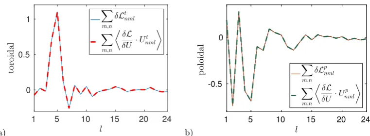
[image:13.595.98.479.127.267.2]>
Figure 1.Verification of the adjoint model. Parameters used in the test:Rm = 60, T = 0.1, ∆t= 10−4
,ε= 10−4
, and (lmax, nmax) = (24,12). a) Toroidal flow coefficients. b) Poloidal flow
coefficients. There is almost exact overlay of the curves depicting the variations inLobtained through two methods.
component of the variationδLis given by
δLρnml=
lnh(BT per)2i −lnh(B
T)2i
ε , (3.1)
whereBT per is the final magnetic field at timeT generated by a given random flow field
plus a small perturbation:U+εUρnml, ρ=t, p. Each component with a different index inn, m, lneeds to be calculated separately using a forward model, whileBT is computed
once without adding perturbations in the random flow field U using a forward model. Second, we calculate the variational derivativeδL/δU projected onto the vector space of
U as in (2.51) by launching the adjoint model only once. The two variations are related by taking the limit of the perturbation amplitudeεto zero:
lim
ε→0δL
ρ nml=
δL δU ·U
ρ nml
, ρ=t, p. (3.2)
We then compare the RHS of (3.1) and (3.2) in spectral space by setting ε to a very small value. All realizations used here have the same initial B0 and U. The test result shows good agreement, see Figure 1.
3.2. A systematic survey identifies the Rmc,min
In a systematic survey, we launch optimisations for various values of the control pa-rameters. The timestep ∆t is set to at most 10−4. The total integration time is mainly
T = 2 except in one optimisation whereT = 2.5 for verification. We have initiated the optimisation loops from either random or previously stored fields. The tolerance level onrtgradually decreases in a refinement approach. For each of these runs, we measure
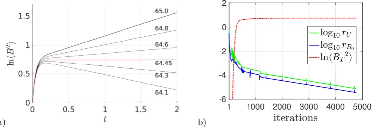
the optimal growth rate γ near the end of the time-interval. Detailed information on all optimisation runs is given in the supplementary materials. In Figure 2, we show the growth rate from multiple optimisation runs, performed at different resolutions in order to finally locate the optimal dynamo threshold at
Rmc,min≈64.45. (3.3)
We refer to this optimal solution as model R1. To ensure that we did not get stuck in a local optimum, we ran an independent optimisation at thisRmc,min, without
10 20 30 40 50 60 70 80 -10
-5 0 5
64 64.5 65
[image:14.595.156.407.127.270.2]-0.2 0 0.2
Figure 2. Main figure: the growth rate as a function of Rm for multiple optimisation runs. Inset figure: the near-zero growth rate as a function of Rm coloured by different resolutions. Orange stars: (lmax, nmax) = (16,8). Green crosses: (lmax, nmax) = (24,12). Purple diamond:
(lmax, nmax) = (24,24).
a) b)
1 1000 2000 3000 4000 5000 -6
-4 -2 0 2
Figure 3.a) Logarithm of the magnetic energyhB2ias a function of time. Red line: data from the optimal solution at Rmc,min = 64.45. Both models R1 and R2 give the same line. Black
line: all models with resolution (lmax, nmax) = (24,12) andrt <10− 4
forRm ∈[64.1,65]. b) The residues and change in the objective as a function of iteration numbers atRm = 64.45 in model R2. Resolutions: (lmax, nmax) = (24,12). Green (middle line): residue for flow fieldU.
Blue (bottom line): residue for seed magnetic fieldB0. Red (dashed line): the logarithm of final
magnetic energy as a function of iterations.
optimisation confirms the location of the threshold. In fact, model R2 is a degenerate solution (see§2.6) of model R1. In Figure 3 a), we show the logarithm of the magnetic energy as a function of time for optimized solutions near the minimal onset of dynamos atRmc,min. We clearly see that the exponential regime is well-established and that the
optimal dynamos are non-oscillatory (Ω = 0 in (2.10)). This indicates T = 2 is long enough to overcome the initial transient. The red curve highlights the run at the opti-mal dynamo threshold. An optimisation run generally needs a few thousand iterations to converge from random initial conditions. It takes about 2 minutes per iteration on 24 cores for (lmax, nmax) = (24,12) resolution, ∆t = 10−4, T = 2. In Figure 3 b), we
[image:14.595.98.474.340.469.2]14 L. Chen, W. Herreman, K. Li, P. W. Livermore, J. W. Luo and A. Jackson
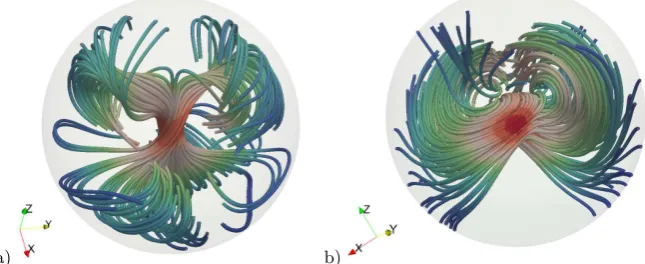
[image:15.595.125.448.131.263.2]a) b)
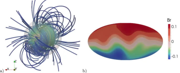
Figure 4.Spatial structures atRmc,min from model R1: a) Streamlines ofU, b) Streamlines
ofBT. Field lines are coloured by local field intensity (red = intense, blue = weak) and indicate a localized structure near the centre. Structures with very small field intensity are not shown here. The plotted domain isr∈[0,1].
3.3. The spatial structure of the optimal solution at Rmc,min
In order to have a complete picture of the optimal dynamo, we analyse the spatial structure of the optimal fields U and BT at Rmc,min in both physical and spectral
space.
3.3.1. Analysis in physical space
In physical space, we show the 3D structure of the streamlines of U and BT from
model R1 in Figure 4 a) and b), field lines are coloured by the local field intensity, small amplitude structures are not shown in the plots for clarity. In Figure 4 a), the field lines appear to be twisting in a twofold manner. We see a drastic increase in the flow speed in the centre. Correspondingly, we also see a strong magnetic field close to the origin in Figure 4 b). Overall we find a quite complex structure in bothU and BT
that apparently lacks reflectional symmetry. This lack of reflectional symmetry was also observed in the optimal dynamos in cubes with perfectly conducting or pseudo-vacuum boundaries (homogeneous cases NNN and TTT in Chen et al. (2015)). However, we observe a rotational symmetry ofπ that the cubic models lack, i.e. only evenm modes are present when the symmetry axis is aligned with the ˆz direction.
We also observe that the velocity and vorticity fields are nearly parallel in the centre, which gives a strong helical motion, shown in Figure 5 a). The magnetic field seems to be enhanced strongly next to the spiral. This is evident when we combine Figures 4 a)-b) and Figure 5 b), where we show the interaction of the flow fieldU and the magnetic field
BT, together with the structure of the vorticity field∇×U. We found the field structure
of BT is mostly dipolar outside the sphere, shown in Figure 6 a) where streamlines of
the magnetic field extend to two radii. The Mollweide map of the radial magnetic field at the sphere surface also confirms the dominant component is dipolar in Figure 6 b). All plots mentioned in this paragraph are based on model R1; model R2 has the same spatial structures up to a rotation.
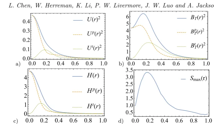
Besides looking directly at the optimal fields, we also want to understand what are the averaged spatial distributions. We introduce a radial distribution of kinetic energy
U(r)2=Ut(r)2+Up(r)2, Uρ(r)2= 1 4π
Z 2π
0
Z π
0
a) b)
Figure 5.a) The velocity field direction (red) and vorticity field direction (black) are nearly parallel withinr60.1. b) Streamlines of the velocity field (orange), the vorticity field (black) and the magnetic field BT (blue) withinr 6 1. The magnetic field is strongest next to the helical fluid motion.
a) b)
Figure 6.a) Streamlines ofBT extended to one radius outside the sphere. b) The Mollweide projection of the radial componentBr ofBT at the surface of the sphere. The vector fieldBT
has been rotated such that the dominant dipole axis is vertical.
BT(r)2, BTt(r)2, B p
T(r)2for the magnetic eigenvector. We also show the radial distribution
of two important quantities: helicity and shear (measured by the absolute maximal strain rate). The toroidal part of the radially varying helicity is given by
Ht(r) = 1 4π
Z 2π
0
Z π
0
Ut·∇×Upsinθdθdφ. (3.5)
SimilarlyHp(r) measures the poloidal part. In total the radial distribution of helicity is
H(r) =Ht(r) +Hp(r). The radial profile of shear is given by
Smax(r) = max φ∈[0,2π], θ∈[0,π]
eig (∇U+∇U⊺)/2. (3.6)
[image:16.595.106.470.319.468.2]16 L. Chen, W. Herreman, K. Li, P. W. Livermore, J. W. Luo and A. Jackson
a)
U(r)2
Up(r)2
Ut(r)2
0.0 0.2 0.4 0.6 0.8 1.0 0.0
0.1 0.2 0.3 0.4
b)
BT(r) 2
BT p(
r)2
Bt(r)2
0.0 0.2 0.4 0.6 0.8 1.0 0
1 2 3 4
5 6
c)
H(r)
Hp(r)
Ht( r)
0.0 0.2 0.4 0.6 0.8 1.0
0 1 2 3 4
d)
Smax(r)
0.0 0.2 0.4 0.6 0.8 1.0 0
[image:17.595.106.450.102.301.2]10 1 20 2 30 3
Figure 7.Radial distributions of the optimal solution. a) Kinetic energy. b) Magnetic energy. c) Helicity. d) Absolute maximal strain rate over all anglesθ, φ.
again showing the alignment of U and ∇×U breaks down within a certain range of
r. We also observe that the magnetic energy in Figure 7 b) almost follows the shear distribution in Figure 7 d). This may at first seem to point to the Omega effect (Moffatt 1983), although in our model the relation between shear and flow is more complex so there is no easy way to relateU andBT throughSmax. For this reason, we cannot give
a definite answer regarding the physics involved in the optimal dynamo. What we can say is that shear (as measured by the absolute maximal strain rate) plays an important role in amplifying the magnetic field.
3.3.2. Analysis in spectral space
In spectral space, we report global measures forU andBT as a function of rotationally
invariant spherical harmonic degreel in Table 2. We introduce the partial sums for the flowU as
Ul=
X
m,n
tnmlUt
nml+snmlUpnml, (3.7)
and similarly for BT l. We notice the l = 1 and l = 3 modes dominate the enstrophy,
and 94% of the enstrophy (squared value) comes from the first three spherical harmonic degrees. The dominant flow field with only these three degrees with lmax = 3 has a
critical magnetic Reynolds number Rmc = 66.29 when the non-dimensional root mean
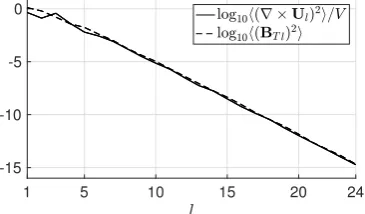
enstrophy is rescaled to 1. This slight increase in the critical point indicates very little influence from higher spherical harmonic degrees in the optimalU. We also notice that the fields have low rms velocities compared to the root mean enstrophy. This indicates that we have strong shear in our optimal flow. In Figure 8, we show power spectra of the optimal root mean enstrophy and magnetic energy as a function of spherical harmonic degree l at Rmc,min. Both models R1 and R2 give the same power spectra. They are
rapidly decaying, which confirms that the spatial resolution we have used is sufficient. Alternatively, we can also analyse each spherical harmonic mode with indexl, m by summing over indicesn. We define the partial sums as
Utml =X
n
tnmlUt
nml, U
pm l =
X
n
snmlUp
1 5 10 15 20 24 -15
[image:18.595.195.378.130.237.2]-10 -5 0
Figure 8.Power spectra of the optimal enstrophyh(∇×Ul)2
i/V and the magnetic energy
h(BT l)2
ias a function of the spherical harmonic degreel.
l= 1 l= 2 l= 3 l= 4 l= 5
h(∇×Ul)2
i/V 0.442 0.130 0.376 0.042 0.006
h(Ul)2
i/V 4.40×10⁻³
2.12×10⁻³
4.77×10⁻³
0.42×10⁻³
0.04×10⁻³
[image:18.595.159.416.404.462.2]h(BT l)2i 1.27 0.62 0.16 0.04 0.02
Table 2.The partial enstrophy, kinetic energy and magnetic energy for the first five spherical harmonic degreeslfrom models R1 and R2, both giving the same value up to three digits.
Up23 Up 0 1 Ut
0
1 Up− 2
2 U
t−2 2 h(∇×Uml )2i/V 0.285 0.231 0.211 0.054 0.046
BTt11 BTp1 1 BTt
1
2 BTp12 BTt− 1 2 h(BTm
l ) 2
i 0.618 0.593 0.384 0.151 0.054
Table 3.Leading components of enstrophy forUm
l and magnetic energy forBTml from model
R1 after rotation and reduction. A summation overnhas been performed for the comparison.
Since the amplitude of eachm mode changes with rotation, we must fix an orientation for the optimalU. We rotate the field in spectral space using Wigner D-matrices such that the rotational symmetry axis is along the ˆz direction and the sum of root mean enstrophy of cos(mφ) modes is maximized. We impose a cut-off of absolute value 0.01 for all spectral coefficients after rotation. The leading spherical harmonic modes are given in Table 3. After a further reduction to keep onlyl 63, the critical magnetic Reynolds number becomes 66.34 when the root mean enstrophy is rescaled to 1, which shows the reduced flow is a good approximation to the full optimum. Capturing 83% of the enstrophy, the optimal flow can be approximated by five spherical harmonic modes:
18 L. Chen, W. Herreman, K. Li, P. W. Livermore, J. W. Luo and A. Jackson
0.5 0.6
0.7 0.8
0.9 1
[image:19.595.162.402.126.247.2]-12 -10 -8 -6 -4 -2 0
Figure 9. Perturbation study of the optimal flow U with l 6 3 using model R1. The cross correlation of the perturbed field and the optimal flow field is given by Cpand the measured
growth rate isγp. Each square represents an independent perturbation onU.
At the level of individual spherical harmonic modes, we notice from Table 3 that the first spherical harmonic mode (l, m) = (1,0) after rotation and reduction has approxi-mately the same enstrophy for both poloidal and toroidal components. It turns out this mode has a normalized helicityHf0
1 = 0.95 where
g
Hm l =hU
m
l ·∇×Uml i/
q
hUml
2
ih(∇×Uml )2i. (3.10) This corresponds to the strong central flow we have shown in Figures 4 a) and 6 a). Other secondary structures are weaker, so the overall normalized helicity for the optimal flow
U is only∼0.65. Helicity is an important measure in fluid dynamics and its significance for dynamo action has been discussed in many places, e.g. review by Moffatt (1983); Gubbins (2008), as well as specific examples given by Livermoreet al.(2007). While our optimal dynamo does have large helicity for some dominant components, helicity alone cannot explain all the optimal structures we have. We also find in Table 3 the equatorial dipole component ofBT is relatively large.
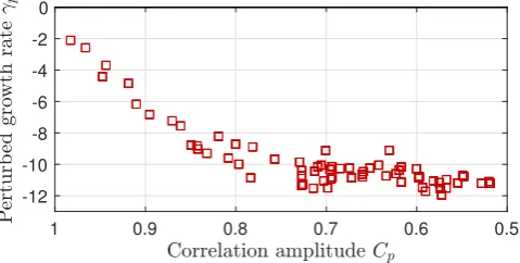
3.4. Perturbation study
In this section, we perform a perturbation study to verify the optimality of the growth rate atRmc,min. A perturbed fieldUper is the optimal field U plus a small portion of a
randomly generated flow field, subsequently rescaled to have a unit enstrophy. We define a correlation amplitude
Cp= h
Uper·Ui
q
h(Uper)2iU2
(3.11)
similar to that in Chenet al.(2015) but only for the dominant modesl63, then launch a forward run withUperand measure the perturbed growth rateγp. The result of multiple
random perturbations is shown in Figure 9. The growth rate rapidly decreases as more perturbations are added toU, which indicates that random perturbations quickly reduce the flow’s optimality.
3.5. Transient growth
a)
0 0.5 1 1.5 2
t
×10-3 0.9996
0.9997 0.9998 0.9999 1 1.0001
h
B
2i
30.22
30.21 30.20
b)
0 0.5 1 1.5 2
t
×10-3 0.9996
0.9997 0.9998 0.9999 1 1.0001
h
B
2i
30.22
[image:20.595.99.466.127.257.2]30.21 30.20
Figure 10. The optimized transient growth. a) Optimized magnetic energy growth for Rm ∈ [30.20,30.22] with optimising time T = 0.001, resolution (lmax, nmax) = (24,12). b)
Comparison of optimized transient growth (red solid line) and R1 (blue dashed line) at the sameRmt,min= 30.21.
then measure the magnetic Reynolds numberRmt,min at which this maximum transient
growth is zero. Numerically, using T = 0.001 and ∆t = 10−5, we find the minimal transient magnetic Reynolds number
Rmt,min= 30.21, (3.12)
see Figure 10 a). No flowU ∈ Euis able to admit magnetic solutions withdhB2i/dt>0
at Rm < Rmt,min. Furthermore, this lower bound Rmt,min also applies to any
time-dependent flow in MHD models that can be approximated by a steady flowU ∈ Eu at
a given instant t. Thus, the value of Rmt,min provides an important physical measure
of the ultimate lower bound for sustaining magnetic energy. Compared with the optimal flow U found with T = 2 in Figure 10 b), we see this magnetic field with maximized transient growth decays more rapidly at later times. This Rmt,min is 53% below the
optimal thresholdRmc,min for sustained dynamo action which is quite different to that
observed by Willis (2012) in the periodic cube. We also find the corresponding optimal flow fieldUtr atRmt,min has equatorial reflectional symmetry.
3.6. Comparison with theoretical bounds
Our magnetic Reynolds numberRmis not the most conventional in dynamo theory, but is the one that relates to the class of enstrophy normalized fieldsU ∈ Eu. We can define
two other magnetic Reynolds numbers using different scales for the flow field:
Rmu=U ∗L∗
η∗ , Rms=
S∗ maxL∗2
η∗ (3.13)
where U∗ is the dimensional rms flow velocity, and S∗
max is the dimensional absolute
maximum strain rate. This allows us to convert the results from root mean enstrophy or shear basedRm to kinetic-energy based (Rmu) and strain rate based (Rms) magnetic
Reynolds numbers:
Rmu=
q
hU2i/V Rm,
Rms=
max
V
eig (∇U+∇U⊺)/2
20 L. Chen, W. Herreman, K. Li, P. W. Livermore, J. W. Luo and A. Jackson
using the non-dimensional optimal flow fieldU. Both models R1 and R2 give the same value. This yields
Rmu= 6.96, Rms= 215. (3.15)
The value of Rmu is very low and close to the values ∼ 12 we have measured in the
cube with unit sizes (Chen et al.2015). According to Proctor (2015), such a low value should be no real surprise since a theoretical lower bound on Rmu does not exist. We
can further check how far we are above theoretical lower bounds using definitions other thanRmu. In particular, we choose three bounds to compare with, they are
(Backus 1958) : Rms> π2,
(Proctor 1977) : Rms>12.29,
(Childress 1969) : RmUmax> π. (3.16)
The Backus/Proctor bounds use a strain-rate based magnetic Reynolds number, and the Childress bound uses the maximum speed of the flow as a typical scale. Using our conventions, we findRms/12.29≈17 andRmUmax/π≈14, which are clearly above the
theoretical limits. This can be attributed to the fact that theoretical bound calculations systematically overestimate the spatial extent of the magnetic fields (Herreman 2016).
Besides the bounds listed above, Proctor (1979) derived a bound for dynamo action that is immediately applicable to our present results. He derived that
D∗> πη
∗2
4L∗ (3.17)
for a sphere of radiusL∗, whereD∗=R e∗
ije∗ijdV∗is proportional to viscous dissipation
ande∗
ij is the dimensional strain rate tensor. Translating this to our notation, we note
that
2D∗= 4 3πL
∗3
S∗2. (3.18)
By dint of the no-slip conditions,S∗=ω∗, and we find immediately that Rm=ω
∗L∗2
η∗ >
√
6
2 ≈0.61. (3.19)
Clearly our dynamo operates well above this bound. Proctor speculated that the best lower bound might be ten times larger than the one given here, and indeed we find that the best dynamo is operating at a value ofRm over one hundred times larger.
3.7. Comparison with other flows
In this section we compare several properties of our optimal flow to some selected models in the literature. We do not include self-consistent dynamos in a spherical shell here due to the complexity of these models (but note that in Christensen & Aubert (2006), the limit for dynamo action isRmu∼60 when the radius is used as the length scale, which is
We first compare the critical magnetic Reynolds numbers for the onset of dynamo action. All the studies we compare with in spheres have used L∗ as the dimensional
radius, but there is little homogeneity in what the scale for the flow field should be (e.g. maximal dimensional speed, rms dimensional speed). In order to compare critical magnetic Reynolds numbers of different dynamo studies, we need to rescale all results to a consistent definition. Denoting Ub the originally reported flow field that was non-dimensionalized using a scale other than [U] =ω∗L∗, we systematically convert Rmd to Rmu,Rm andRmsrespectively:
Rmu=
q
hUb2i/V Rmd, Rm=
q
h(∇×Ub)2i/V Rmd,
Rms=
max
V
eig (∇Ub +∇Ub⊺)/2Rmd=SbmaxRmd. (3.20)
The comparison of critical magnetic Reynolds numbers and the rescaling factors in (3.20) are shown in Table 4. We see our optimal flowU has improved the existing lower bound on the critical Rm of DJ t2s2 by at least a factor of 3. TheRmu for our optimal flow U is also significantly lower than the others. The trade-off of this is that the maximal strain rate remains comparable to DJ flows (we comparedSmaxandSbmax(hUb
2
i/V)1/2). It is not yet clear how to reduce local shear and global shear at the same time. As for the transient growth, our ultimate lower boundRmt,min= 30.21 is at least 2 times lower than
the critical transient magnetic Reynolds number (Rmt) for selected flows from Livermore
& Jackson (2004), shown in Table 5.
Additionally, we also compare important properties of the optimal flow such as helicity, energy ratio and maximum speed in Table 6. We use the poloidal/toroidal kinetic energy and enstrophy given by
EP/ET =h(Up)2i/h(Ut)2i, ωP2/ωT2=h(∇ ×Up)2i/h(∇ ×Ut)2i, (3.21)
where the superscript pandt denote the poloidal and toroidal component of flow field respectively. The choice of scale [U] does not influence the energy ratios, so we use the same notation for all models. The total helicity in the sphere and the hemispherical helicity for flowsUb are given by
hHbiV = 3
4πhUb · ∇ ×Ubi, hHbiV2 =
3 2π
Z 1
0
Z 2π
0
Z π
2
0
b
U· ∇ ×Ub r2sinθ dθdφdr. (3.22) We use the same formula without the hat symbol for the flow field that has been non-dimensionalized using scale [U] = ω∗L∗. From Table 6 it seems that there is no clear
pattern on these measured values across different dynamo models. We observe that for our optimal flow the poloidal enstrophy to toroidal enstrophy ratio is roughly the same as poloidal kinetic energy to toroidal kinetic energy ratio.
3.8. Comparison with the cubic model
It is of interest to compare our present results to our previous results in a cube (Chenet al.
2015). When mixed boundary conditions were used, the best dynamo had Rmc,min =
22 L. Chen, W. Herreman, K. Li, P. W. Livermore, J. W. Luo and A. Jackson
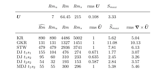
Rmu Rm Rms rmsU Smax
U 7 64.45 215 0.108 3.33
d
Rm Rmu Rm Rms rmsUb Sbmax rms∇×Ub
KR 890 890 4486 5002 1 5.62 5.04
GKR 131 131 1327 1451 1 11.08 10.13
STW 479 479 2936 3741 1 7.81 6.13
DJt1s1 155 104 476 274 0.671 1.77 3.07
DJt1s2 95 60 310 233 0.635 2.45 3.26
DJt2s2 54 32 193 153 0.587 2.84 3.57
[image:23.595.114.449.132.279.2]MDJt1s2 55 55 300 296 1 5.38 5.46
Table 4.A comparison of critical magnetic Reynolds numbers between our optimised flow (top row) and those reported in the literature (bottom section), the rescaling factor rms (· · ·) is equivalent to (h(· · ·)2
i/V)1/2
, see (3.14), (3.20) and Appendix B for more definitions.
Utr KR STW MDJt1s2
Rmt 30.21 80 83 62
Table 5.The critical transient magnetic Reynolds number for the optimal transient flowUtr and selected flows from Livermore & Jackson (2004), converted using (h(∇×Ub)2
i/V)1/2
as the rescaling factor.
hHiV hHiV
2 maxV |
U| ωP2
/ωT2 EP/ET
U 0.07 0.08‡ 0.69 1.885 1.824
hHbiV hHbiV
2 maxV |b
U| ωP2
/ωT2 EP/ET
KR 0 0.210 1.96 0.149 0.017
GKR 0 2.078 2.58 8.117 1
STW 0 0.362 2.38 0.088 0.015
DJt1s1 1.969 1.969 1.12 0.630 0.592
DJt1s2 0 1.380 1.07 0.838 0.425
DJt2s2 1.992 1.992 0.94 0.791 0.679
MDJt1s2 0 2.906 1.64 0.662 0.254
Table 6. Properties of the flow fields that can generate a dynamo (see Appendix B for the definition of flows). ‡: We choose the hemisphere with the larger value of helicity when the
symmetry axis is aligned with the ˆzaxis.
all chords present in both the sphere and the cube. For the sphere of radiusLit is clear thatE{l2}= 4L2= (E{l})2, whereas in the cube, we find
E{L2}= 5/3 (3.23)
conditions. These compare to the values in the sphere we report here when converted usingE{l2}= 4L2 ofRm
c,min= 258 for insulating boundary conditions.
A complementary way of comparing is to imagine that we are given a unit volume of electrically conducting fluid and consider the two possible geometrical arrangements at our disposal: a cube and a sphere. Obviously the size of the sphere (using radius R) is 4π/3R3 = 1, thusR= (3/(4π))1/3≈0.62. We choose a common length scale, which is unity for the cube and for the sphere must be measured in these units. We previously referred our Rm to the radius, but the present lengthscale inflates the length units by (0.62)−1.When we reinterpret our present value for Rm on this length scale we have a new value for Rm of 64.45/0.622 ≈168, now above all the cubic results. Probably we have taken this analysis as far as is sensible, but we speculate that the extra roughness of the boundaries present in the cube might be responsible for additional shearing in the optimal flow that then appears to be a better dynamo.
4. Conclusions
In this study, we have found the optimal kinematic dynamo in a sphere with no-slip and insulating boundary conditions. The enstrophy based minimal critical Rmc,min for
the onset of a dynamo is 64.45. Compared to other known dynamo models, our optimal dynamo has lowered the criticalRmat least by a factor of 3. The rms speed is much lower compared to the global shear magnitude or root mean enstrophy in the system. The op-timal flow field atRmc,minhas a rotational symmetry of order 2 and a very concentrated
helical structure near the centre. This indicates that a localised helix plus secondary twofold spirals are favourable for the onset of a kinematic dynamo in a sphere. The dom-inant spherical harmonic modes are (l,|m|) = (1,0),(2,2),(3,2), when the rotational symmetry axis is aligned with ˆz axis. The optimal flow structures near the boundary do not play a significant role. Therefore, we expect that the use of other boundary conditions for the flow, such as free-slip boundary conditions, will not lowerRmc,minby much. The
magnetic field at the dynamo onset has mainly dipolar structures. With respect to the rotational symmetry axis of U, the fastest growing magnetic field eigenmode has only oddmmodes. We also find the minimal critical magnetic Reynolds number for transient growth Rmt,min = 30.21, indicating any time-dependent flows cannot lower the critical
magnetic Reynolds number below 30.21.
Our optimisation method is designed to identify the best dynamo, but it does not answer the question “why are these flows so efficient in generating dynamos?” quanti-tatively. Obtaining and analysing the optimal flow as we have done here is just a first step, while providing understanding what makes them optimal physically is a much more relevant but rather difficult second step. In the supplementary material of this article, we have provided both the spectral coefficients and field values on grids for the optimal flow field and the associated magnetic eigenvector for possible follow-up studies. Since our polynomial basis is not standard, we also include aMathematicafile that allows one
to generate the optimal flow in physical space and on arbitrarily fine grids.
24 L. Chen, W. Herreman, K. Li, P. W. Livermore, J. W. Luo and A. Jackson
5. Acknowledgements
This work was supported by the ETH Research Commission through grant ETH-08 13-2 for which we are grateful. Additional support by SNF grants 200020 143596 and 200021 163163 is acknowledged. We would like to thank Dr. Ashley Willis and Prof. Michael Proctor for valuable discussions.
Appendix A. Orthonormal bases of toroidal/poloidal vector fields
In this section we give the definitions of our Galerkin bases and show how to project a vector field onto these bases.
A.1. The Poloidal-toroidal expansions
The poloidal-toroidal decomposition for the flow field is
Ut(r, θ, φ) = X
l,m,n
Tnml
1
rsinθ f
l n(r)
∂Ym l
∂φ θˆ−
1
r f
l n(r)
∂Ym l
∂θ φˆ
, (A 1)
Up(r, θ, φ) = X
l,m,n
Snml
l(l+ 1)
r2 g
l
n(r)Ylmˆr+
1
r ∂gl
n(r)
∂r ∂Ym
l
∂θ θˆ+
1
rsinθ ∂gl
n(r)
∂r ∂Ym
l
∂φ φˆ
,
(A 2) where fnl, gnl are radial functions and Ylm are the spherical harmonics. The field
de-composition for B follows similar definitions. There are in total 2nmaxlmax(lmax+ 2)
spectral coefficients for each vector field. For input and output, these coefficients are stored in memory as a one dimensional array. In the optimisation process, the memory is distributed to at least lmax number of cores. In this model, we use fully normalized
real spherical harmonics. The spherical harmonics are defined as
Ylm(θ, φ) =Nlm
(
cos(mφ)Pbm
l (cosθ), ifm>0,
sin(|m|φ)Pbl|m|(cosθ), ifm <0, (A 3)
wherePbm
l (cosθ) are the associated Legendre functions, defined as
b
Plm(x) = (−1)m(1−x2) m
2 d
m
dxmP˜n(x), (A 4)
where ˜Pn(x) is a Legendre polynomial of x, and Nlm =
q(2−δ
0m)(2l+1)
4π
(l−|m|)! (l+|m|)! is a normalization factor such that we have the orthonormality condition for the spherical harmonics:
Z 2π
0
Z π
0
Ylm(θ, φ)Y˜lm˜(θ, φ) sinθ dθdφ=δl˜lδmm˜. (A 5)
The derivatives of spherical harmonics satisfy dYm
l
dφ =−mY
−m
l , sinθ
dYm l
dθ =−(l+ 1)ˆa
m
l Ylm−1+laˆml+1Ylm+1, (A 6) where ˆam
l =
q(l+|m|)(l−|m|)
![Figure 10. The optimized transient growth. a) Optimized magnetic energy growth forComparison of optimized transient growth (red solid line) and R1 (blue dashed line) at thesameRm ∈ [30.20, 30.22] with optimising time T = 0.001, resolution (lmax, nmax) = (2](https://thumb-us.123doks.com/thumbv2/123dok_us/1930753.152607/20.595.99.466.127.257/optimized-transient-optimized-forcomparison-optimized-transient-optimising-resolution.webp)