Generalised Network Autoregressive Processes and the GNAR package

White Rose Research Online URL for this paper:

http://eprints.whiterose.ac.uk/151108/

Version: Accepted Version

Article:

Knight, Marina Iuliana orcid.org/0000-0001-9926-6092, Leeming, Kathryn, Nason, G.P. et

al. (1 more author) (Accepted: 2019) Generalised Network Autoregressive Processes and

the GNAR package. Journal of Statistical Software. ISSN 1548-7660 (In Press)

[email protected] https://eprints.whiterose.ac.uk/ Reuse

Items deposited in White Rose Research Online are protected by copyright, with all rights reserved unless indicated otherwise. They may be downloaded and/or printed for private study, or other acts as permitted by national copyright laws. The publisher or other rights holders may allow further reproduction and re-use of the full text version. This is indicated by the licence information on the White Rose Research Online record for the item.

Takedown

If you consider content in White Rose Research Online to be in breach of UK law, please notify us by

MMMMMM YYYY, Volume VV, Issue II. doi: 10.18637/jss.v000.i00

Generalised Network Autoregressive Processes and

the

GNAR

package

Marina Knight

University of York

Kathryn Leeming

University of Bristol

Guy Nason

University of Bristol

Matthew Nunes

University of Bath

Abstract

This article introduces the GNAR package, which fits, predicts, and simulates from a powerful new class of generalised network autoregressive processes. Such processes consist of a multivariate time series along with a real, or inferred, network that provides information about inter-variable relationships. The GNAR model relates values of a time series for a given variable and time to earlier values of the same variable and of neighbouring variables, with inclusion controlled by the network structure. The GNAR

package is designed to fit this new model, while working with standard tsobjects and theigraphpackage for ease of use.

Keywords: multivariate time series, networks, missing data, network time series.

1. Introduction

Increasingly within the sciences, networks and network methodologies are being used to an-swer research questions. Such networks might be observed, such as connections in communi-cation network or information flows within, or they could be unobserved: inferred networks that can explain a process or effect. Given the increase in the size of data sets, it may also be useful to infer a network from data to efficiently summarise the data generating process. We consider time series observations recorded at different nodes of a network, or graph.

Our GNAR package (Leeming, Nason, Nunes, and Knight 2019) and its novel generalised

network autoregressive (GNAR) statistical models focus on partnering a network with a multivariate time series and modelling them jointly. One can find an association network,

see, e.g., Chapter 7 of Kolaczyk (2009), or Granger causality network, e.g., Dahlhaus and

Networks can provide strong information about the dependencies between variables. Within our generalised network autoregressive (GNAR) model, each node depends on its previous values as in the univariate autoregressive framework, but also may depend on the previous val-ues at its neighbours, neighbours of neighbours, and so on. Our GNAR modelling framework is flexible, allowing for different types of network, networks that change their structure over time (time-varying networks), and also can be powerfully applied in the important practical situation where the time series feature missing observations.

Driven in part by the increased popularity and recent research activity in the field of statistical network analysis, there has been a concurrent growth in software for analysing such data. An exhaustive list of these packages is beyond the scope of this article, but we review some relevant ones here.

Existing software in this area predominantly focusses on the various models for network-structured data. In the static network setting, these include packages dedicated to latent

space network models, such as collpcm (Wyse, Ryan, and Friel 2017), HLSM (Adhikari,

Junker, Sweet, and Thomas 2018), latentnet(Krvitsky, Handcock, Shortreed, Tantrumet al.

2018b) amongst others; exponential random graph models and their variants, for example

ergm (Handcock, Hunter, Butts et al.2018),GERGM(Denny, Wilson, Cranmer, Desmarais, and Bhamidi 2018) orhergm(Schweinberger, Handcock, and Luna 2018); and block models in

e.g.,blockmodels(Leger 2015). For dynamic networks, packages for time-varying equivalents

of these network models are also available, see e.g., thetergmpackage (Krvitsky, Handcock,

Hunter, Goodreauet al. 2018a) or dynsbm(Matias and Miele 2018). There are also a multi-tude of more general packages for network analysis, e.g., for network summary computation or implementations of methodology in specific applications of interest.

Despite this, software dedicated to the analysis of time series and other processes on

net-works is sparse. A number of packages implement epidemic (e.g., SIR) models of disease

spread, notably epinet (Groendyke, Welch, and Hunter 2018), EpiLM/EpiLMCT (Warriyar

and Deardon 2018; Almutiry, Warriyar, and Deardon 2018) and hybridModels (Marquez, Grisi-Filho, and Amaku 2018); these use transmission rates to model processes as opposed

to temporal and network dependence through time series models as in GNAR. Similarly,

the NetOrigin software (Manitz and Harbering 2018) is dedicated to source estimation for propagation processes on networks, rather than fitting time series models. Packages such asnetworkTomography (Blocker, Koullick, and Airoldi 2014) deal with time-varying models

for (discrete) count processes or flows on links of afixed routing network; thetnam package

(Leifeld and Cranmer 2017) fits models using spatial (and not network-node) dependence.

Both of these are in contrast to the GNAR package, which implements time series models

which account for known time-varying network structures.

Other packages can implicitly develop network-like structured time series models through

pe-nalised or constrained variable selection, such asautovarCore(Emerencia 2018),nets(

Brown-lees 2017),sparsevar(Vazoller, Frattarolo, and Billio 2016), as well as thevarspackage (Pfaff

2008). Packages that take a graphical modelling approach to the dependence structure within

time series include gimme (Lane, Gates, Fisher, Molenaar et al. 2019), graphicalVAR (

Ep-skamp 2018),mgm(Haslbeck 2019),mlVAR(Epskamp, Deserno, and Bringmann 2019), and

sparseTSCGM(Abegaz and Wit 2016). These approaches also differ fundamentally from the

GNAR models since the network is constructed during analysis, as opposed toGNAR, which

specifically incorporates information on the network structure into the model a priori. The

models and this existing class of techniques.

Section 2 introduces our model, and demonstrates how GNAR can be used to fit network

models to simulated network time series in Section 2.4. Order selection and prediction are

discussed in Section3, which includes an example of how to use BIC to select model order for a

wind speed network time series in Section3.2. An extended example, concerning constructing

a network to aid GDP forecasting, is presented in Section 4. Section 5 discusses different

network modelling options that could be chosen, and presents a summary of the article. All

results were calculated using version 3.5.1 of the statistical softwareR(RCore Team(2017)).

2. Network time series processes

We assume that our multivariate time series follows an autoregressive-like model at each node, depending both on the previous values of the process at that node, and on neighbouring nodes at previous time steps. These neighbouring nodes are included as part of the network structure, as defined below.

2.1. Network terminology and notation

Throughout we assume the presence of one or more networks, or graphs, associated with the observed time series. Each univariate time series that makes up the multivariate time series occurs, or is observed at, a node, or location on the graph(s). These nodes are connected by a set of edges, which may be directed, and/or weighted.

We denote a graph by _G = (_K,_E), where _K = _{1, ..., N_} is the set of nodes, and _E is the

set of edges. A directed edge from node i ∈ K to j ∈ K is denoted i j, and an

un-directed edge between the nodes is denoted i ! j. The edge set of a directed graph is

E=_{(i, j) :i j;i, j_{∈ K}}, and similarly for the set of un-directed edges.

Stage-r neighbourhoods

We introduce the notion of neighbours and stage-neighbours in the graph structure as follows;

for a subset A _{⊂ K} the neighbour set of A is given by _N(A) = _{j _{∈ K}/A : i j;i _∈ A_}.

These are the first neighbours, or stage-1 neighbours of A. The rth stage neighbours of a

node i∈ K are given by N(r)_{(i) =N {N}(r−1)_(i)}/[{∪r−1

q=1N(q)(i)} ∪ {i}], for r = 2,3, ... and

N(1)_{(i) =N({i}).}

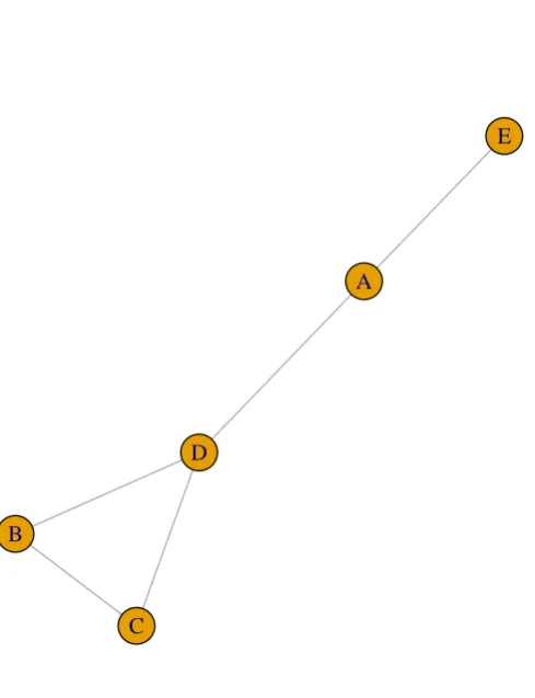
Figure1 shows an example graph, where node E has stage-1 neighbour A, stage-2 neighbour

D, and stage-3 neighbours B and C. Neighbour sets for this example include N(1)_{(D) =}

{A, B, C_}, and _N(3)_{(E) = {B, C}. In the time-varying network setting, a subscript t is}

added to the neighbour set notation.

Connection weights

Each network can have connection weights ω ∈ [0,1] associated with every pair of nodes.

This connection weight can depend on the size of the neighbour set and also encodes any

edge-weight information. Formally, the values of the connection weights from a nodei_{∈ K}to

its stage-r neighbour j∈ N(r)_{(i) will be the reciprocal of the number of stage-r neighbours;}

ωi,j = |N(r)(i)|−1, where | · | denotes the cardinality of a set. In Figure 1 the connection

necessarily symmetric, even for an un-directed graph. We note that this choice of these inverse distance weights is one of many possibilities, and some other means of creating connection weights could be used.

When the edges are weighted, or have a distance associated with them, we use the concept

of distance to find the shortest path between two vertices. Let the distance from node i

to ℓ be denoted di,ℓ ∈ R+, and if there is an un-normalised weight between these nodes,

denote this µi,ℓ ∈ R+. To find the length of connection between a node i and its stage-r

neighbour, k, we sum the distances on the paths with r edges from i to k and take the

minimum (note that there are no paths with fewer edges thanr askis a stage-r neighbour).

If the network includes weights rather than distances, we find the shortest r length path

wheredi,ℓ = µ−i,ℓ1. Then the connection weights between node iand its stage-r neighbour k

are either ωi,k = d−_i,k1{Pℓ∈N(r)_(i)d−_i,ℓ1}−1 for distances, or ωi,k = µi,k{Pℓ∈N(r)_(i)µi,ℓ}−1 for a

network with weights. This definition means that all nodes will have connection weights that sum to one for any non-empty neighbour set, whether they are in a sparse or dense part of the graph.

Edge or node covariates

A further important innovation permits a covariate that can be used to encode edges effects

(or nodes) into certain types. Our covariate will take C _∈N_{discrete values and be indexed}

by c. A more general covariate could be considered, but we wish to keep our notation simple

in the definition that follows. For example, in an epidemiological network we might have two edge types: one that carries information about windborne spread of infection and the other carries information about identified direct infections. The covariates do not change our

neighbour sets or connection weight definitions, so we have the property P

q∈N(r)_(i)

C

P

c=1

ωi,q,c = 1

for all i_{∈ K} and r_∈N_{such thatN}(r)_{(i) is non-empty.}

2.2. The generalised network autoregressive model

Consider an N _×1 vector of nodal time series,Xt= (X1,t, . . . , XN,t)′, whereN is considered

fixed. Our aim is to model the dependence structure within and between the nodal series

using the network structure provided by (potentially time-varying) connection weights, ω.

For each node i_{∈ {}1, . . . , N_} and time t _{∈ {}1, . . . , T_}, our generalised autoregressive model

of order (p,[s])_∈N_×Np

0 forXt is

Xi,t = p

X

j=1 



αi,jXi,t−j +

C

X

c=1

sj

X

r=1

βj,r,c

X

q∈N_t(r)(i)

ω_i,q,c(t) Xq,t−j





+ui,t, (1)

wherep_∈N_{is the maximum time lag, [s] = (s1, . . . , sp) andsj ∈}N_{0 is the maximum stage of}

neighbour dependence for time lagj, with N_{0 =}N_{∪ {0}, Nt}(r)_{(i) is the rth stage neighbour}

set of node i at time t, ω_i,q,c(t) _∈ [0,1] is the connection weight between node i and node q

at timet if the path corresponds to covariate c. Here, we consider a sum from one to zero

to be zero, i.e.: P0

r=1(·) := 0. The αi,j ∈ R are ‘standard’ autoregressive parameters at lag

j for node i. The βj,r,c ∈ R correspond to the effect of the rth stage neighbours, at lag j,

to achieve process stationarity over the network. Here the noise, _{ui,t}, is assumed to be

independent and identically distributed at each node i, with mean zero and variance σ2_i.

Our model meaningfully enhances that of the arXiv publication Knight, Nunes, and Nason

(2016) by now additionally including different autoregressive parameters, connection weights

at each node and, particularly, parametersβ that depend on covariates. Note that the IID

assumption on the noise_{ui,t}could of course be relaxed to include correlated innovations.

We note that crucially, the time-dependent network topology is integral to the model parametri-sation through the use of time-varying weights and neighbours. These features yield a model that is sensitive to the network structures and captures contemporaneous as well as

autore-gressive relationships, as defined by equation (1). The network should therefore be viewed

not as an estimable quantity, but as a time-dependent known structure.

In the GNAR model, the network may change over time, but the covariates stay fixed. This means that the underlying network can be altered over time, for example, to allow for nodes to drop in and out of the series but model fitting can still be carried out. Practically, this

is extremely useful, as shown by the example in Section 4. Our model allows for the α

parameters may be different at each node, however the interpretation of the network regression

parameters,βj,r,c, is the same throughout the network.

A more restrictive version of the above model is the global-α GNAR(p,[s]) model, which

has the same autoregressive covariate at each node, where the αi,j are replaced by αj. This

defines a process with the same behaviour at every node, with differences being present only due to the graph structure.

2.3. GNAR network example

Networks in the GNAR package are stored in a list with two components edges and dist.

The edges component is itself a list with N slots each containing a vector whose entries

are indices to their neighbouring nodes. For example, if 3!4 denotes an undirected edge

between nodes 3 and 4 then the vector edges[[3]] will contain a 4 and edges[[4]] will

contain a3. If the network is undirected this will mean that each edge is ‘double counted’ in

summary information. A directed edge 3 4 would be listed in edges[[3]]as a 4, but not

edges[[4]]if there is no edge in the opposite direction. The distcomponent is of the same

format as edges, and contains the distances corresponding to the edge links, if they exist.

For example, in an un-weighted setting, the connection weights are such that all neighbours

of a node have equal effect on the node. This is achieved by setting all entries of the dist

component to one, and the software calculates the connection weight from these. A GNAR

network is stored in aGNARnet object, and an object can be checked using the is.GNARnet

function. The S3 methodsplot,print, andsummary are available for GNARnetobjects.

Figure 1 shows an example that is stored as a GNARnet object called fiveNet and can be

reproduced using

R> library("GNAR") R> library("igraph")

R> plot(fiveNet, vertex.label = c("A", "B", "C", "D", "E"))

The basic structure of the GNARnet object is, as usual, displayed with

●

●

●

●

●

A

B

C D

E

Figure 1: An example un-directed, un-weighted graph with five nodes labelled A to E.

GNARnet with 5 nodes and 10 edges of equal length 1

Converting a network to GNARnet form

Our GNARnet format integrates with other methods of specifying a network via a set of

functions that generate aGNARnetfrom others, such as anigraphobject.

An igraph object can be converted to and from the GNARnet structure using the functions

igraphtoGNAR and GNARtoigraph, respectively. For example, starting with the fiveNet GNARnetobject,

R> fiveNet2 <- GNARtoigraph(net = fiveNet) R> summary(fiveNet2)

R> fiveNet3 <- igraphtoGNAR(fiveNet2) R> all.equal(fiveNet, fiveNet3)

[1] TRUE

whereas the reverse conversion would be performed as

R> g <- make_ring(10) R> print(igraphtoGNAR(g))

GNARnet with 10 nodes

edges:1--2 1--10 2--1 2--3 3--2 3--4 4--3 4--5 5--4 5--6 6--5 6--7 7--6 7--8 8--7 8--9 9--8 9--10 10--1 10--9

edges of each of length 1

We can also use theGNARtoigraphfunction to extract graphs involving higher-order neighbour

structures, for example, creating a network of third-order neighbours.

In addition to interfacing withigraph, we can convert betweenGNARnetobjects and adjacency

matrices using functionsas.matrixandmatrixtoGNAR. We can produce an adjacency matrix

for thefiveNetobject with

R> as.matrix(fiveNet)

[,1] [,2] [,3] [,4] [,5]

[1,] 0 0 0 1 1

[2,] 0 0 1 1 0

[3,] 0 1 0 1 0

[4,] 1 1 1 0 0

[5,] 1 0 0 0 0

and an example converting a weighted adjacency matrix to aGNARnetobject is

R> adj <- matrix(runif(9), ncol = 3, nrow = 3) R> adj[adj < 0.3] <- 0

R> print(matrixtoGNAR(adj))

GNARnet with 3 nodes

edges:1--1 1--2 1--3 2--1 2--3 3--1 3--2 edges of unequal lengths

2.4. Example: GNAR model fitting

ThefiveNet network has a simulated multivariate time series associated with it of class ts

called fiveVTS. The pair together are a network time series. The object can be loaded in

from GNAR models: GNARfit and the predict method, respectively. These make use of

the familiar R command lm, since the GNAR model can be essentially re-formulated as a

linear model, as we shall see in Section 3 and Appendix B. As such, least squares variance

/ standard error computations are also readily obtained, although other, e.g. HAC-type variance estimators could also be considered for GNAR models.

Suppose we wish to fit the global-αnetwork time series model GNAR(2,[1,1]), a model with

four parameters in total. We can fit this model with the following code.

R> data("fiveNode")

R> answer <- GNARfit(vts = fiveVTS, net = fiveNet, alphaOrder = 2, + betaOrder = c(1, 1))

R> answer

Model:

GNAR(2,[1,1])

Call:

lm(formula = yvec ~ dmat + 0)

Coefficients:

dmatalpha1 dmatbeta1.1 dmatalpha2 dmatbeta2.1

0.20624 0.50277 0.02124 -0.09523

In this fit, the global autoregressive parameters are ˆα1 ≈ 0.206 and ˆα2 ≈ 0.021 and the β

network parameters are ˆβ1,1,1 ≈0.503 and ˆβ2,1,1 ≈ −0.095. Also, the network edges only have

one type of covariate so C =c= 1. We can just look at one node. For example, the model

at node A is

XA,t= 0.206XA,t−1+0.503(XE,t−1+XD,t−1)/2+0.021XA,t−2−0.095(XE,t−2+XD,t−2)/2+uE,t.

The model coefficients can be extracted from aGNARfitobject using the coef function as is

customary. The GNARfit object returned by GNARfit function also has methods to extract

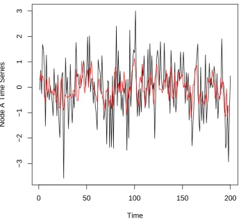
fitted values and the residuals. For example, Figure 2 shows the first node time series and

the residuals from fitting the model. Figure2was produced by

R> plot(fiveVTS[, 1], ylab = "Node A Time Series") R> lines(fitted(answer)[, 1], col = 2)

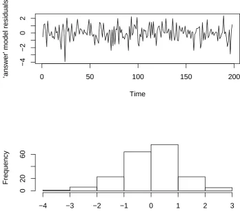
Alternatively, we can examine the associated residuals:

R> myresiduals <- residuals(answer)[, 1] R> layout(matrix(c(1, 2), 2, 1))

R> plot(ts(residuals(answer)[, 1]), ylab = "`answer' model residuals")

R> hist(residuals(answer)[, 1], main = "", xlab = "`answer' model residuals")

By altering the input parameters in the GNARfit function, we can fit a range of different

Time

Node A Time Ser

ies

0 50 100 150 200

−3

−2

−1

0

1

2

3

Figure 2: Time series of first node (black) with fitted values from ‘answer’ model overlaid in red.

2.5. Example: GNAR data simulation on a given network

The following example demonstrates network time series simulation using the network in

Figure1.

Model(a)is a GNAR(1,[1]) model with individualαparameters, (αA,1, αB,1, αC,1, αD,1, αE,1) =

(0.4,0,₋0.6,0,0), and the same β parameter throughout, β1 = 0.3. Model (b) is a global-α

GNAR(2,[2,0]) model with parameters α1 = 0.2, β1,1 = 0.2, β1,2 = 0.3 and α2 = 0.3. Both

simulations are created using standard normal noise whose standard deviation is controlled

using thesigmaargument.

R> set.seed(10)

R> fiveVTS2 <- GNARsim(n = 200, net = fiveNet,

+ alphaParams = list(c(0.4, 0, -0.6, 0, 0)), betaParams = list(c(0.3)))

By fitting an individual-alpha GNAR(1,[1]) model to the simulated data with the fiveNet

Time

‘answ

er' model residuals

0 50 100 150 200

−4

−2

0

2

‘answer' model residuals

Frequency

−4 −3 −2 −1 0 1 2 3

0

20

60

Figure 3: Residual plots from ‘answer’ model fit. Top: Time series; Bottom: Histogram.

-0.6, 0, 0 and 0.3. This agreement does not come as a surprise given that we show theoretical

consistency for parameter estimators (see Appendix B).

R> print(GNARfit(vts = fiveVTS2, net = fiveNet, alphaOrder = 1, + betaOrder = 1, globalalpha = FALSE))

Model: GNAR(1,[1])

Call:

lm(formula = yvec ~ dmat + 0)

Coefficients:

dmatalpha1node1 dmatalpha1node2 dmatalpha1node3 dmatalpha1node4

dmatalpha1node5 dmatbeta1.1

0.02249 0.24848

Repeating the experiment for the GNAR(2, [2, 0]) Model (b), the estimated parameters are

again similar to the generating parameters:

R> set.seed(10)

R> fiveVTS3 <- GNARsim(n = 200, net = fiveNet, + alphaParams = list(rep(0.2, 5), rep(0.3, 5)), + betaParams = list(c(0.2, 0.3), c(0)))

R> print(GNARfit(vts = fiveVTS3, net = fiveNet, alphaOrder = 2, + betaOrder = c(2,0)))

Model:

GNAR(2,[2,0])

Call:

lm(formula = yvec ~ dmat + 0)

Coefficients:

dmatalpha1 dmatbeta1.1 dmatbeta1.2 dmatalpha2

0.2537 0.1049 0.3146 0.2907

Alternatively, we can use thesimulateS3 method forGNARfitobjects to simulate time series

associated to a GNAR model, for example

R> fiveVTS4 <- simulate(GNARfit(vts = fiveVTS2, net = fiveNet, alphaOrder = 1, + betaOrder = 1, globalalpha = FALSE), n = 200)

2.6. Missing data and changing connection weights with GNAR models

Standard multivariate time series models, including vector autoregressions (VAR), can have significant problems in coping with certain types of missingness and imputation is often used, see Guerrero and Gaspar (2010), Honaker and King (2010), Bashir and Wei (2016). While in VAR modelling successful solutions have been found to cope with specific missingness

scenarios, such as implemented in the gimme R package. However, if a variable has e.g.

block missing data, the coefficients corresponding that variable can be difficult to calculate, and impossible if their partner variable is missing at cognate times. In addition, due to

computational burden gimmeis limited to modelling a single time lag. A key advantage of

connections and weightings need altering accordingly. Again, using the graph in Figure 1, consider the situation where node A does not have any data recorded. Yet, we want to pre-serve the stage-2 connection between D and E, and the stage-3 connection between E and both B and C. To do this, we do not redraw the graph and remove node A and its con-nections, instead we reweight the connections that depend on node A. As node A does not

feature in the stage-2 or stage-3 neighbours of E, the connection weightsωE,D, ωE,B, ωE,C do

not change, but the connection weightωE,A drops to zero in the absence of observation from

node A. Similarly, the stage-1 neighbours of D are changed without A, soωD,A drops to zero

and the other two connection weights from node D increase accordingly;ωD,B=ωD,C = 0.5.

Missing data of this kind is handled automatically by theGNAR functions using customaryNA

missing data values present in thevts(vector time series) component of the overall network

time series. For example, inducing some (artificial) missingness in thefiveVTSseries, we can

still obtain estimates of model parameters:

R> fiveVTS0 <- fiveVTS

R> fiveVTS0[50:150, 3] <- NA

R> nafit <- GNARfit(vts = fiveVTS0, net = fiveNet, alphaOrder = 2, + betaOrder = c(1, 1))

R> layout(matrix(c(1, 2), 2, 1))

R> plot(ts(fitted(nafit)[, 3]), ylab = "Node C fitted values") R> plot(ts(fitted(nafit)[, 4]), ylab = "Node D fitted values")

As shown in Figure4, after removing observations from the time series at node C, its

neigh-bour, node D, still has a complete set of fitted values.

2.7. Stationarity conditions for a GNAR process with fixed network

Theorem 1 Given an unchanging network, G, a sufficient condition for the GNAR model (1) to be stationary is

p

X

j=1

|αi,j|+

C

X

c=1

sj

X

r=1

|βj,r,c|

!

<1 ∀i∈1, ..., N. (2)

The proof of Theorem1can be found in Appendix A.

For the global-α model this condition reduces to

p

X

j=1

|αj|+

C

X

c=1

sj

X

r=1

|βj,r,c|

!

<1. (3)

We can explore these conditions using the GNARsim function. The following example uses

parameters whose absolute value sums to greater than one and then we calculate the mean over successive time periods. The mean increases rapidly indicating nonstationarity.

R> set.seed(10)

R> fiveVTS4 <- GNARsim(n = 200, net = fiveNet,

+ alphaParams = list(rep(0.2, 5)), betaParams = list(c(0.85))) R> c(mean(fiveVTS4[1:50, ]), mean(fiveVTS4[51:100, ]),

Time

Node C fitted v

alues

0 50 100 150 200

−1.0

0.0

1.0

Time

Node D fitted v

alues

0 50 100 150 200

−1.0

0.5

1.5

Figure 4: Fitted values of global-α GNAR(1,[1]) fit to the ‘fiveVTS’ data, with observations

50–150 removed from node C. Fitted values: Top: Node C; Bottom: Node D.

[1] -120.511 -1370.216 -15725.884 -180319.140

2.8. Benefits of our model and comparisons to others

Conditioned on a given network fixed in time and with a known (time-dependent) weight- and neighbourhood structure, the GNAR model can be mathematically formulated as a specific restricted VAR model, where the restrictions are imposed by the network and thus impact

model parametrisation, as mathematically encoded by equation (1). This is explored in more

depth in Appendix B and contrasts with a VAR model where any restrictions can only be

imposed on the parameters themselves.

An unrestricted VAR model with dimensionnhas_O(n2_{) parameters, whereas a GNAR model}

with known network (usually) hasO(n) parameters, and a global-α GNAR model can have

O(1) parameters. The large, and rapidly increasing, number of parameters in VAR often make

to mitigate those challenges. Further, the large number of VAR parameters usually mean that it fits multivariate time series well, but then performs poorly in out-of-sample prediction. An

example of this is shown in Section4.

Our model has similarities with the network autoregression introduced byZhu, Pan, Li, Liu,

and Wang(2017), motivated by social networks.

In our notation, the Zhuet al. (2017) model can be written as a special case as

Xi,t =β0+Zi⊤γ+ p

X

j=1 

αjXi,t−j+βj

X

q∈N(1)_(i)

ωiXq,t−j



+ui,t, (4)

whereβ0 is a global intercept term,Ziis a vector of node-specific covariates with

correspond-ing parameters γ, ωi is the reciprocal of the out-degree of node i, and the innovations are

independent and identically distributed, with zero mean, such that var(ui,t) = σ2. Hence,

the Zhu et al. (2017) model without intercept and node-specific covariates is a special case

of our GNAR model, with max

j∈{1,...,p}sj = 1, i.e. dependencies limited to stage-1 immediate

neighbours, and un-weighted edges.

Our model is designed to deal with a time-varying network, and our βj,r,c parameters can

include general edge-based covariate information. A further important advantage is that our

GNAR model in Section 2.2 can express dependence on stage-r neighbour sets for any r.

An earlier model with similarities to the generic network autoregression is the Dynamic

Bayesian Network (DBN) model considered in Spencer, Hill, and Mukherjee (2015). Their

model can be written as

Xi,t =β0,i+

X

q∈N(1)_(i)

βi,qXq,t−1+ui,t, (5)

where β0,i is a node-specific intercept term, the other β parameters describe the network

autoregression, and ui,t ∼ N(0, σi2). The DBN model is also a constrained VAR model,

but with no univariate autoregression terms, and the network autoregression only includes

the stage-1 neighbours. Unlike our model and the Zhu et al. (2017) model, there are no

restrictions on the parameters other than parameters only being present when there is an

edge between two nodes. The Spenceret al. (2015) framework does not allow for a range of

networks, as their underlying network is assumed to be a Directed Acyclic Graph. With these assumptions, the network and parameters are inferred by considering potential predictors for

each node in turn. A key difference between our model and theSpenceret al.(2015) model is

that we assume that the behaviour of connected nodes is the same throughout the network,

whereas the DBN model allows for differentβ parameters for different connections, including

allowing a change of sign.

The benefits of the GNAR model compared to these, and other models, include the ability to deal with a time-changing network, missing observations, and using network information

to reduce the number of parameters. As detailed in Section 2.6, we can incorporate missing

3. Estimation

In modelling terms, our GNAR model is a linear model and we employ standard techniques such as least squares estimation to fit them and to provide statistically consistent estimators,

as verified in Appendix B. An important practical consideration for fitting GNAR models is

the choice of model order. Specifically, how do we selectp ands?

3.1. Order selection

We use the Bayesian information criterion (BIC) proposed by Schwarz (1978) to select the

GNAR model order. Under the assumption of a constant network, and that the innovations are independent and identically distributed white noise with bounded fourth moments, this

criterion is consistent, as shown in Lütkepohl(2005). The BIC allows us to select both the

lag and neighbourhood orders simultaneously by selecting the model with smallest BIC from a set of candidates.

For a general candidate GNAR(p,[s]) model withN nodes, the BIC is given by

BIC(p,s) = ln_|Σˆp,s|+T

−1_{Mln(T), (6)}

where ˆΣp,s=T

−1_Uˆ′_{Uˆ, ˆU is the residual matrix from the NAR(p,[s]) fit, and M is the}

number of parameters. In the general case M =N p+CPp

j=1sj, and in the global-α model

M =p+CPp

j=1sj. The covariance matrix estimate, ˆΣp,s, is also the maximum likelihood

estimator of the innovation covariance matrix under the assumption of Gaussian innovations.

GNAR enables us to easily compute the BIC for any model by using the BIC method for

GNARfit objects. For example, on the default model fitted by GNARfit, and an alternative model that additionally includes second-order neighbours at the first lag into the model, we can compare their BICs by

R> BIC(GNARfit())

[1] -0.003953124

R> BIC(GNARfit(betaOrder = c(2, 1)))

[1] 0.02251406

Whilst we focus on the BIC for model selection for the remainder of this article, the GNAR

package also include functionality for the Akaike information criterion (AIC) proposed by

Akaike(1973) as

AIC(p,s) = ln|Σˆp,s|+ 2T

−1_{M, (7)}

where ˆΣp,s is as defined in equation (6) and M is again the number of model parameters.

Similar to above, the AIC can be obtained by using the code

R> AIC(GNARfit())

R> AIC(GNARfit(betaOrder = c(2, 1)))

[1] -0.05994387

Similar to the BIC, the model with the lowest AIC is preferred. Note that the likelihood of

the data associated to the model fit can also be obtained using e.g.,logLik(GNARfit()).

Various models can be tried to obtain a good fit whilst, naturally, attending to the usual aspects of good model fitting, such as residual checks. A thorough simulation study that

displays the numerical performance of our proposed method appears in Section 4.5 ofLeeming

(2019).

3.2. Model selection on a wind network time series

GNAR incorporates the data suite vswind that contains a number of R objects pertaining

to 721 wind speeds taken at each of 102 weather stations in England and Wales. The suite

contains the vector time series vswindts, the associated network vswindnet, a character

vector of the weather station location names in vswindnamesand coordinates of the stations

in the two column matrix vswindcoords. The data originate from the UK Met Office site

http://wow.metoffice.gov.ukand full details can be found in the vswindhelp file in the

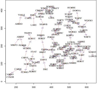
GNARpackage. Figure5shows a picture of the meteorological station network with distances

created by

R> oldpar <- par(cex = 0.75) R> windnetplot()

R> par(oldpar)

We investigate fitting a network time series model. We first fit a simple GNAR(1,[0]) model

using a singleα, followed by an equivalent model with potentially individually distinct αs

R> BIC(GNARfit(vts = vswindts, net = vswindnet, alphaOrder = 1, + betaOrder = 0))

[1] -233.3848

R> BIC(GNARfit(vts = vswindts, net = vswindnet, alphaOrder = 1, + betaOrder = 0, globalalpha = FALSE))

[1] -233.1697

Interestingly, the model with the single α gives the better fit, as judged by BIC. The single

αmodel with alphaOrder = 2and betaOrder = c(0, 0)gives a lower BIC of₋243, so we

investigate this next. Note that this model also gives the lowest AIC score. In particular,

we explore a set of GNAR(2,[b1, b2]) models with b1, b2 ranging from zero to 14 using the

following code:

200 300 400 500 600 0 100 200 300 400 0.62 0.51 0.46 0.51 0.5 0.27 0.5 0.21 0.27 0.51 0.13 0.13 0.13 0.42 0.15 0.34 0.34 0.4 0.38 0.25 0.59 0.23 0.31 0.48 _0.63 0.24 0.65 0.47 0.44 0.62 0.18 0.6 0.45 0.43 0.06 0.16 0.48 0.22 0.36 0.29 0.45 0.41 0.5 0.59 0.19 0.15 0.16 0.30.24 0.08 0.34 0.14 0.23 0.55 0.1 0.4 0.36 0.43_0.4 0.35 0.31

0.060.19 0.29 0.18 0.42 0.24 0.31 0.04 0.17 0.22 0.18 0.27 0.27 0.22 0.24 0.21 0.15 0.72 0.57 0.47 0.62 0.21 0.52 0.39 0.28 0.25 0.29 0.2 0.42 0.4 0.16 0.11 0.39 0.05 0.09 0.3 0.07 0.31 0.44 0.35 ● ● ● ● ● ● ● ● ● ● ● ● ● ● ● ● ● ● ● ● ● ● ● ● ● ● ● ● ● ● ● ● ● ● ● ● ● ● ● ● ● ● ● ● ● ● ● ● ● ● ● ● ● ● ● ● ● ● ● ● ● ● ● ● ● ● ● ● ● ● ● ● ● ● ● ● ● ● ● ● ● ● ● ● ● ● ● ● ● ● ● ● ● ● ● ● ● ● ● ● ● ● VALLE CAPEL RHYL CROSB HAWAR _LEEK: EMLEY WOODF NOTTI SCAMP WADDI CRANW DONNA CONIN WAINF

ABERD _LAKE SHAWB

COTTE WITTE HOLBE MARHA WEYBO ABERP TRAWS SENNY SHOBD HEREF PERSH COLES CHURC BEDFO WATTI MILFO PEMBR MUMBL FILTO LITTL BRIZE BENSOHIGH NORTH ANDRE SHOEB CHIVE LISCO

ST AT LYNEH

LARKH BOSCO

MIDDL

ODIHASOUTH_CHARL HEATH KENLE GRAVE LANGD MANST CAMBO CULDR CARDI PLYMO DUNKE YEOVI ISLE HURN WIGHT THORN SOLEN SHOREHERST EAST ROCHD ELMDO RINGW BRIST LUTON GATWI LONDO HUMBE EAST STANS MILDE FAIRF MONKS SUTTO COVEN WISLE KEW G ETON: SOUTH WIGHT WINTE MANCH NORTH BERRY LAKEN SPEKE SOUTH EXETE SOUTH

Figure 5: Plot of the wind speed network. Blue numbers are relative distances between sites; labels are the site name.

+ for(b2 in 0:14)

+ BIC.Alpha2.Beta[b1 + 1, b2 + 1] <- BIC(GNARfit(vts = vswindts, + net = vswindnet, alphaOrder = 2, betaOrder = c(b1, b2))) R> contour(0:14, 0:14, log(251 + BIC.Alpha2.Beta),

+ xlab = "Lag 1 Neighbour Order", ylab = "Lag 2 Neighbour Order")

The results of the BIC evaluation for incorporating different and deeper neighbour sets, at

lags one and two, are shown in the contour plot in Figure6. The minimum value of the BIC

occurs in the bottom-right part of the plot, where it seems incorporating five or sixth-stage neighbours for the first time lag is sufficient to achieve the minimum BIC, and incorporating further lag one stages does not reduce the BIC. Moreover, increasing the lag two neighbour sets beyond first stage neighbours would appear to increase the BIC for those lag one neighbour stages greater than five (the horizontal contour at 0 in the bottom right hand corner of the plot). A fit of a possible model is

Lag 1 Neighbour Order

Lag 2 Neighbour Order

0 0.2

0.2

0.2

0.4 0.6

0.8 1

1.2

0 2 4 6 8 10 12 14

0

2

4

6

8

10

12

14

Figure 6: Contour plot of BIC values for the two-lag autoregressive model incorporating

b1-stage andb2-stage neighbours at time lags one and two. Values shown are log(251 + BIC)

to display clearer contours.

+ betaOrder = c(5, 1)) R> goodmod

Model:

GNAR(2,[5,1])

Call:

lm(formula = yvec ~ dmat + 0)

Coefficients:

dmatalpha1 dmatbeta1.1 dmatbeta1.2 dmatbeta1.3 dmatbeta1.4

0.56911 0.10932 0.03680 0.02332 0.02937

dmatbeta1.5 dmatalpha2 dmatbeta2.1

We investigated models with alphaOrder equal to two, three, four and five, but with no

neighbours. As judged by BIC, alphaOrder = 3 gives the best model. We could extend

the example above to investigate differing stages of neighbours at time lags one, two and three. However, a more comprehensive BIC investigation would examine all combinations of neighbour sets over a large number of time lags. This would be feasible, but computationally intensive for a single CPU machine, but could be coarse-grain parallelized. Further analysis would proceed with model diagnostic checking and further modelling as necessary.

3.3. Constructing a network to aid prediction

Whilst some multivariate time series have actual, and sometimes obvious, networks associated with them, our methodology can be useful for series without a clear or supplied network. We propose a network construction method that uses prediction error, but note here that our scope is not to estimate an underlying network, but merely to find a structure that is useful in the task of prediction. Here, we use a prediction error measure, understood as the sum of

squared differences between the observations and the estimates: PN

i=1(Xi,t−Xˆi,t)2.

ThepredictS3 method for GNAR models takes an inputGNARfitmodel object and from this

predicts the nodal time series at the next timepoint, similar to the S3 method for theArima

class. This allows for a ‘ex-sample’ prediction evaluation. Thepredictfunction outputs the

prediction as a vector. For example, to predict the series at the last timepoint

R> prediction <- predict(GNARfit(vts = fiveVTS[1:199,], net = fiveNet, + alphaOrder = 2, betaOrder = c(1, 1)))

R> prediction

Time Series: Start = 1 End = 1

Frequency = 1

Series 1 Series 2 Series 3 Series 4 Series 5 1 -0.6427718 0.2060671 0.2525534 0.1228404 -0.8231921

For a small-dimensional multivariate series, any and all potential un-weighted networks can

be constructed and the corresponding prediction errors compared using thepredictmethod.

Next, we consider the larger data setting where it is computationally infeasible to investigate

all possible networks. Erdős-Rényi random graphs can be generated with N nodes, and a

fixed probability of including each edge between these nodes, see Chapter 11 of Grimmett

(2010) for further details. The probability parameter controls the overall sparsity of the graph.

Many random graphs of this type can be created, and then our GNAR model can be used for within-sample prediction. The prediction error can then be used to identify networks that aid prediction. We give an example of this process in the next section.

4. OECD GDP: Network structure aids prediction

We obtained the annual gross domestic product (GDP) growth rate time series for 35 countries

from the OECD website1. The series covers the years 1961–2013, but not all countries are

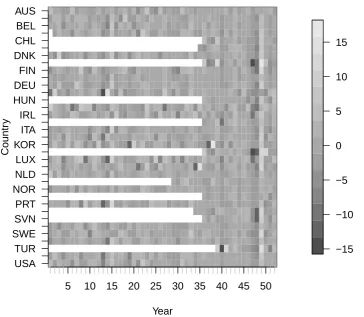
included from the start. The values are annual growth rates expressed as a percentage change compared to the previous year. We differenced the time series for each country to remove the gross trend.

We use the first T = 52 time points and designate each of the 35 countries as nodes to

investigate the potential of modelling this time series using a network. In this data set 20.8% (379 out of 1820) of the observations were missing due to some nodes not being included from the start. We model this by changing the network connection weights as described in

Section 2.6. In this example, we do not use covariate information, so C= 1. The pattern of

missing data along with the time series values is shown graphically in Figure 7, produced by

the following code.

R> library("fields")

R> layout(matrix(c(1, 2), nrow = 1, ncol = 2), widths = c(4.5, 1)) R> image(t(apply(gdpVTS, 1, rev)), xaxt = "n", yaxt = "n",

+ col = gray.colors(14), xlab = "Year", ylab = "Country")

R> axis(side = 1, at = seq(from = 0, to = 1, length = 52), labels = FALSE, + col.ticks = "grey")

R> axis(side = 1, at = seq(from = 0, to = 1, length = 52)[5*(1:11)], + labels = (1:52)[5*(1:11)])

R> axis(side = 2, at = seq(from = 1, to = 0, length = 35), + labels = colnames(gdpVTS), las = 1, cex = 0.8)

R> layout(matrix(1))

R> image.plot(zlim = range(gdpVTS, na.rm = TRUE), legend.only = TRUE, + col = gray.colors(14))

4.1. Finding a network to aid prediction

This section considers the case where we observe data up tot= 51, and then wish to predict

the values for each node att= 52. We begin by exploring ‘within-sample’ prediction att= 51,

and identify a good network for prediction. We use randomly generated Erdős-Rényi graphs

using theGNAR functionseedToNet. To demonstrate this, theGNARpackage contains the

gdp data and a set of seed values, seed.nos so that the random graphs can be reproduced

for use with the time series objectgdpVTShere.

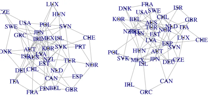
R> net1 <- seedToNet(seed.no = seed.nos[1], nnodes = 35, graph.prob = 0.15) R> net2 <- seedToNet(seed.no = seed.nos[2], nnodes = 35, graph.prob = 0.15) R> layout(matrix(c(2, 1), 1, 2))

R> par(mar=c(0,1,0,1))

R> plot(net1, vertex.label = colnames(gdpVTS), vertex.size = 0) R> plot(net2, vertex.label = colnames(gdpVTS), vertex.size = 0)

Figure 8 shows two of these random graphs.

As well as investigating which network works best for prediction, we also need to identify the number of parameters in the GNAR model. Initial analysis of the autocorrelation function at each node indicated that a second-order autoregressive component should be sufficient, so

Year

Countr

y

5 10 15 20 25 30 35 40 45 50 USA

TUR SWE SVN PRT NOR NLD LUX KOR ITA IRL HUN DEU FIN DNK CHL BEL AUS

−15 −10 −5 0 5 10 15

Figure 7: Heat plot (greyscale) of the differenced time series, where the initial white space indicates missing time series observations.

sets at each time lag. The GNAR models are: GNAR(1,[0]), GNAR(1,[1]), GNAR(2,[0,0]),

GNAR(2,[1,0]), GNAR(2,[1,1]), GNAR(2,[2,0]), GNAR(2,[2,1]), and GNAR(2,[2,2]), each

fitted as individual-α and global-α GNAR models, giving sixteen models in total.

For the GDP example, we simulate 10,000 random un-directed networks, each with connection probability 0.15, and predict using the GNAR model with the orders above. Hence, this example requires significant computation time (about 90 minutes on a desktop PC), so only a segment of the analysis is included in the code below. For computational reasons, we first divide through by the standard deviation at each node so that we can model the residuals

as having equal variances at each node. The function seedSim outputs the sum of squared

differences between the prediction and original values, and we use this as our measure of prediction accuracy.

R> gdpVTSn <- apply(gdpVTS, 2, function(x){x / sd(x[1:50], na.rm = TRUE)}) R> alphas <- c(rep(1, 2), rep(2, 6))

● ● ● ● ● ● ● ● ● ● ● ● ● ● ● ● ● ● ● ● ● ● ● ● ● ● ● ● ● ● ● ● ● ● ● AUS AUT BEL CAN CHL CZE DNK EST FIN FRA DEU GRC HUN ISL IRL ISR ITA JPN KOR LVA LUX MEX NLD NZL NOR POL PRT SVK SVN ESP SWE CHE TUR GBR USA ● ● ● ● ● ● ● ● ● ● ● ● ● ● ● ● ● ● ● ● ● ● ● ● ● ● ● ● ● ● ● ● ● ● ● AUS AUT BEL CAN CHL CZE DNK EST FIN FRA DEU GRC HUN ISL IRL ISR ITA JPN KOR LVA LUX MEX NLD NZL NOR POL PRT SVK SVN ESP SWE CHE TUR GBR USA

Figure 8: Erdős-Rényi random graphs constructed from the first two elements of the

seed.nosvariable with 35 nodes and connection probability 0.15.

+ c(2, 2))

R> seedSim <- function(seedNo, modelNo, globalalpha){

+ net1 <- seedToNet(seed.no = seedNo, nnodes = 35, graph.prob = 0.15) + gdpPred <- predict(GNARfit(vts = gdpVTSn[1:50, ], net = net1,

+ alphaOrder = alphas[modelNo], betaOrder = betas[[modelNo]], + globalalpha = globalalpha))

+ return(sum((gdpPred - gdpVTSn[51, ])^2)) + }

R> seedSim(seedNo = seed.nos[1], modelNo = 1, globalalpha = TRUE)

[1] 23.36913

R> seedSim(seed.nos[1], modelNo = 3, globalalpha = TRUE)

R> seedSim(seed.nos[1], modelNo = 3, globalalpha = FALSE)

[1] 18.96766

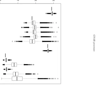
Prediction error boxplots over simulations from all sixteen models and 10,000 random

net-works are shown in Figure 9 (accompanying code not shown due to significant computation

time). The global-α model resulted in lower prediction error in general, so we use this version

of the GNAR model. For GNAR(1,[0]) and GNAR(2,[0,0]), the first and third model in

Figure 9 the “boxplots” are short horizontal lines as the results for each graph are

identi-cal, as no neighbour parameters are fitted. As the other global-α models are nested within

it, we select the randomly generated graph that minimises the prediction error for global-α

GNAR(2,[2,2]); this turns out to be the network generated fromseed.nos[921].

R> net921 <- seedToNet(seed.no = seed.nos[921], nnodes = 35, + graph.prob = 0.15)

R> layout(matrix(c(1), 1, 1))

R> plot(net921, vertex.label = colnames(gdpVTS), vertex.size = 0)

The network generated fromseed.nos[921]is plotted in Figure10, where all countries have

at least two neighbours, with 97 edges in total. This “921” network was constructed with GDP prediction in mind, so we would not necessarily expect any interpretable structure in our found network (and presumably, there were other networks with not too dissimilar predictive power). However, the USA, Mexico and Canada are extremely well-connected with eight, eight and six edges, respectively. Sweden and Chile are also well-connected, with eight and seven edges, respectively. This might seem surprising, but, e.g., the McKinsey Global

Institute MGI Connectedness Index, see Manyika, Lund, Bughin, Woetzel, Stamenov, and

Dhingra (2016), ranks Sweden and Chile 18th and 45th respectively out of 139 countries, and each country is most connected within their regional bloc (Nordic and South America, respectively). Each of these edges, or subgraphs of the “921” network could be tested to find a sparser network with a similar predictive performance, but we continue with the full chosen network here.

Using this network, we can select the best GNAR order using the BIC.

R> res <- rep(NA, 8) R> for(i in 1:8){

+ res[i] <- BIC(GNARfit(gdpVTSn[1:50, ],

+ net = seedToNet(seed.nos[921], nnodes = 35, graph.prob = 0.15), + alphaOrder = alphas[i], betaOrder = betas[[i]]))

+ }

R> order(res)

[1] 6 3 4 7 8 5 1 2

R> sort(res)

GNAR

p

ro

ce

sse

s

10 15 20 25

GNAR(1,[0])

GNAR(1,[1])

GNAR(2,[0,0])

GNAR(2,[1,0])

GNAR(2,[1,1])

GNAR(2,[2,0])

GNAR(2,[2,1])

GNAR(2,[2,2])

GNAR(1,[0]) g−α

GNAR(1,[1]) g−α

GNAR(2,[0,0]) g−α

GNAR(2,[1,0]) g−α

GNAR(2,[1,1]) g−α

GNAR(2,[2,0]) g−α

GNAR(2,[2,1]) g−α

GNAR(2,[2,2]) g−α

re

9:

P

re

d

ic

tion

error

b

oxp

lots

at

t

=

51

ov

er

10,000

ran

d

omly

ge

n

erate

d

n

et

w

orks

u

sin

g

an

d

d

iffe

re

n

t

GNAR

mo

d

els,

wh

ere

‘g-α

’

in

d

ic

ate

s

a

glob

al-α

GNAR

mo

d

●

●

●

●

● ●

●

● ●

●

●

● ●

●

●

●

●

●

●

● ●

●

●

●

●

●

●

● ●

● ●

● ●

●

●

AUS

AUT _BEL

CAN CHL

CZE

DNK

EST FIN

FRA

DEU

GRC HUN

ISL

IRL

ISR

ITA

JPN

KOR

LVA LUX

MEX

NLD

NZL

NOR

POL

PRT

SVK SVN

ESP SWE

CHE TUR

GBR

USA

Figure 10: Randomly generated un-weighted and un-directed graph over the OECD countries

that minimises the prediction error att= 51 using GNAR(2,[2,2]).

The model that minimised BIC in this case was the sixth model, GNAR(2,[2,0]), a model with

two autoregressive parameters and network regression parameters on the first two neighbour sets at time lag one.

4.2. Results and comparisons

We use the previous section’s model to predict the values att= 52 and compare its prediction

errors to those found using standard AR and VAR models. The GNAR predictions are found

by fitting a GNAR(2,[2,0]) model with the chosen network (corresponding toseed.nos[921])

to data up tot= 51, and then predicting values at t= 52. We first normalise the series, and

then compute the total squared error from the model fit.

R> gdpVTSn2 <- apply(gdpVTS, 2, function(x){x / sd(x[1:51], na.rm = TRUE)}) R> gdpFit <- GNARfit(gdpVTSn2[1:51,], net = net921, alphaOrder = 2,

R> summary(gdpFit)

Call:

lm(formula = yvec2 ~ dmat2 + 0)

Residuals:

Min 1Q Median 3Q Max

-3.4806 -0.5491 -0.0121 0.5013 3.1208

Coefficients:

Estimate Std. Error t value Pr(>|t|) dmat2alpha1 -0.41693 0.03154 -13.221 < 2e-16 *** dmat2beta1.1 -0.12662 0.05464 -2.317 0.0206 * dmat2beta1.2 0.28044 0.06233 4.500 7.4e-06 *** dmat2alpha2 -0.33282 0.02548 -13.064 < 2e-16 ***

---Signif. codes: 0 '***' 0.001 '**' 0.01 '*' 0.05 '.' 0.1 ' ' 1

Residual standard error: 0.8926 on 1332 degrees of freedom (23 observations deleted due to missingness)

Multiple R-squared: 0.1859, Adjusted R-squared: 0.1834 F-statistic: 76.02 on 4 and 1332 DF, p-value: < 2.2e-16

GNAR BIC: -62.86003

R> sum((predict(gdpFit) - gdpVTSn2[52, ])^2)

[1] 5.737203

The fitted parameters of this GNAR model were ˆα1 ≃ −0.42,βˆ1,1 ≃ −0.13,βˆ1,2 ≃0.28, and

ˆ

α2 ≃ −0.33.

We compared our methods with results from fitting an AR model individually to each node

using theforecast.ar()andauto.arima()functions from version 8.0 of the CRANforecast

package, for further details seeHyndman and Khandakar(2008). Due to our autocorrelation

analysis from Section4.1we set the maximum AR order for each of the 35 individual models

to bep= 2. Conditional on this, the actual order selected was chosen using the BIC.

R> library("forecast")

R> arforecast <- apply(gdpVTSn2[1:51, ], 2, function(x){

+ forecast(auto.arima(x[!is.na(x)], d = 0, D = 0, max.p = 2, max.q = 0, + max.P = 0, max.Q = 0, stationary = TRUE, seasonal = FALSE, ic = "bic", + allowmean = FALSE, allowdrift = FALSE, trace = FALSE), h = 1)$mean + })

R> sum((arforecast - gdpVTSn2[52, ])^2)

Model # Parameters Prediction error

GNAR(2,[2,0]) 4 5.7

Individual AR(2) 38 8.1

VAR(1) 199 26.2

Table 1: Estimated prediction error of differenced real GDP change at t = 52 for all 35

countries.

Our VAR comparison was calculated using version 1.5–2 of the CRAN package vars, Pfaff

(2008). The missing values at the beginning of the series cannot be handled with current

software, so are set to zero. The number of parameters in a zero-mean VAR(p) model is

of order pN2_{. In this particular example, the dimension of the observation data matrix is}

T×N, withT <2N, so only a first-order VAR can be fitted. We fit the model using theVAR

function and then use therestrictfunction to reduce dimensionality further, by setting to

zero any coefficient whose associated absolutet-statistic value is less than two.

R> library("vars")

R> gdpVTSn2.0 <- gdpVTSn2

R> gdpVTSn2.0[is.na(gdpVTSn2.0)] <- 0

R> varforecast <- predict(restrict(VAR(gdpVTSn2.0[1:51, ], p = 1, + type = "none")), n.ahead = 1)

This results in forecast vectors for each node, so we extract the point forecast (the first element of the forecast vectors) and compute the prediction error as follows

R> getfcst <- function(x){return(x[1])}

R> varforecastpt <- unlist(lapply(varforecast$fcst, getfcst)) R> sum((varforecastpt - gdpVTSn2.0[52, ])^2)

[1] 26.19805

Our GNAR model gives a lower prediction error than both the AR and VAR results, reducing

the error by 29% compared to AR and by 78% compared to VAR. Table1 summarises these

results and also shows the number of parameters fitted. It is clear that GNAR is particularly parsimonious.

We repeat the procedure above to perform analysis based upon two-step ahead forecasting. In this case, a different network minimises the prediction error for model GNAR(2,[2,2]). However, the BIC step identified that the GNAR(2,[0,0]) model had the best fit, which is a model that does not include network regression parameters.

R> gdpVTSn3 <- apply(gdpVTS, 2, function(x){x / sd(x[1:50], na.rm = TRUE)}) R> gdpPred <- predict(GNARfit(gdpVTSn2[1:50,], net = net921, alphaOrder = 2, + betaOrder = c(0, 0)), n.ahead=2)

R> sum((gdpPred[1,] - gdpVTSn3[51, ])^2)

[1] 11.7874

Model Prediction error at t= 51 Prediction error att= 52

GNAR(2,[0,0]) 11.8 8.1

Individual AR(2) 18.6 11.3

VAR(1) 115.0 120.4

Table 2: Estimated prediction error of differenced real GDP change at t= 51,52, for all 35

countries.

[1] 8.067577

R> arforecast <- apply(gdpVTSn3[1:50, ], 2, function(x){

+ forecast(auto.arima(x[!is.na(x)], d = 0, D = 0, max.p = 2, max.q = 0, + max.P = 0, max.Q = 0, stationary = TRUE, seasonal = FALSE, ic = "bic", + allowmean = FALSE, allowdrift = FALSE, trace = FALSE), h = 2)$mean + })

R> sum((arforecast[1,] - gdpVTSn3[51, ])^2)

[1] 18.56074

R> sum((arforecast[2,] - gdpVTSn3[52, ])^2)

[1] 11.31722

R> gdpVTSn3.0 <- gdpVTSn3

R> gdpVTSn3.0[is.na(gdpVTSn3.0)] <- 0

R> varforecast <- predict(restrict(VAR(gdpVTSn3.0[1:50, ], p = 1, + type = "none")), n.ahead = 2)

R> getfcst <- function(x){return(x[,1])}

R> varforecastpt <- matrix(unlist(lapply(varforecast$fcst, getfcst)), + nrow=2, ncol=35)

R> sum((varforecastpt[1,] - gdpVTSn3[51,])^2)

[1] 114.9876

R> sum((varforecastpt[2,] - gdpVTSn3[52,])^2)

[1] 120.4467

Table2shows that the GNAR model is again the best performing, although in the two-step

ahead prediction the fitted model is a special case of GNAR model with no neighbourhood parameters.

Results in Tables1and2indicate that the VAR model works particularly poorly here, despite

p, it can capture. In addition, we were unable to find software to fit VAR models with for missing data at the start of a series.

We end this section by noting that using Erdős-Rényi graphs are not the only type of network that could be used to aid prediction. As suggested by a referee, models such the Chung-Lu

model (Aiello, Chung, and Lu 2001; Chung and Lu 2002) could also be used to simulate

random networks for this task; these graphs would allow for more flexible network generation, for example using node-specific connection probabilities proportional to a country’s size.

5. Discussion and summary

TheGNAR package can be used to model network time series using a network autoregressive

structure. Estimation under the proposed model is informed by the, potentially time-varying, structure of the network, assumed known. Network time series models are in an early stage of development, but there is enormous potential, especially as network data are increasingly being collected and analysed in many fields. As far as possible, we attempt to integrate our methods with existing valuable R functionality, such as its linear modelling capability and thefit/ summary/ predictmethods that are familiar with Rusers.

Within our model a network is formed using edges of all covariates simultaneously, and the

connection weights of this single network can be calculated e.g. as described in Section2.1.2.

Another approach is to consider a separate network for each covariate, and then calculate connection weights for each of these networks. This would result in different (known)

weight-ings,ω, and consequently different fitted coefficients,β. The single network approach is more

appropriate for sparse networks and when different types of edge are closely related. In com-parison, when covariates relate completely separate link information between the nodes, use of different networks would be appropriate.

When covariates are present, the neighbour set structure is more complex, as different edge

types can be included in a path between nodes. For example, in a network with event and

proximal edges, network paths between stage-2 neighbours could include edges event-event,

event-proximal / proximal-event, or proximal-proximal. These different types of path could

be represented separately in the model using additional β parameters. We note that the

number of such parameters would increase greatly for large covariate cardinality C or high

neighbour set stagesj, so, in these cases, the large number of additional parameters may not

enhance the model. Our model permits regression on any non-empty stage neighbour set, so

models with highsj can be fitted. For large sj, the neighbour sets may not be scientifically

interpretable so small sj is recommended, to favour parsimony and interpretability.

Trend is another factor that can seriously affect modelling and estimation, just as in the regular time series situation. However, trend can be successfully modelled and estimated by

using second-generation wavelet (lifting) techniques before stochastic modelling, as inNunes,

Knight, and Nason(2015).

With the option of having different covariates and high order neighbourhood structures

in-cluded, our GNAR model as presented in Section 2 is incredibly flexible. In this article a

References

Abegaz F, Wit E (2016). TSCGM: Sparse Time Series Chain Graphical Models. R package

version 2.5, URLhttp://CRAN.R-project.org/package=SparseTSCGM.

Adhikari S, Junker B, Sweet T, Thomas AC (2018).HLSM: Hierarchical Latent Space Network

Model. Rpackage version 0.8, URLhttp://CRAN.R-project.org/package=HLSM.

Aiello W, Chung F, Lu L (2001). “A random graph model for power law graphs.”Experimental

Mathematics,10(1), 53–66.

Akaike H (1973). “Information Theory and An Extension of the Maximum Likeihood

Princi-ple.” InProc. 2nd International Symposium on Information Theory, pp. 267–281. Academiai

Kiado, Budapest, Hungary.

Almutiry V, Warriyar KV, Deardon R (2018). EpiLMCT: Continuous Time Distance-Based

and Network Based Individual Level Models for Epidemics. Rpackage version 1.1.2, URL

http://CRAN.R-project.org/package=EpiLMCT.

Bashir F, Wei HL (2016). “Handling Missing Data in Multivariate Time Series Using a

Vec-tor AuVec-toregressive Model Based Imputation (VAR-IM) Algorithm.” InProc. 24th

Mediter-ranean Conference on Control and Automation (MED), pp. 611–616. IEEE, Athens, Greece.

Blocker AW, Koullick P, Airoldi E (2014). networkTomography: Tools for Network

Tomography. R package version 0.3, URL http://CRAN.R-project.org/package=

networkTomography.

Brockwell PJ, Davis RA (2006). Time Series: Theory and Methods. 2nd edition.

Springer-Verlag, New York.

Brownlees C (2017). nets: Network Estimation for Time Series. Rpackage version 0.9, URL

http://CRAN.R-project.org/package=nets.

Chung F, Lu L (2002). “Connected components in random graphs with given expected degree

sequences.” Annals of Combinatorics,6(2), 125–145.

Dahlhaus R, Eichler M (2003). “Causality and Graphical Models for Time Series.” In

PJ Green, NL Hjort, , S Richardson (eds.), Highly Structured Stochastic Systems., pp.

115–137. Oxford University Press, Oxford.

Denny MJ, Wilson JD, Cranmer S, Desmarais BA, Bhamidi S (2018). GERGM:

Estima-tion and Fit Diagnostics for Generalized Exponential Random Graph Models. R package

version 0.13.0, URLhttp://CRAN.R-project.org/package=GERGM.

Emerencia A (2018). autovarCore: Automated Vector Autoregression Models and Networks.

Rpackage version 1.0-4, URL http://CRAN.R-project.org/package=autovarCore.

Epskamp S (2018). graphicalVAR: Graphical VAR for Experience Sampling Data. Rpackage

version 0.2.2, URLhttp://CRAN.R-project.org/package=graphicalVAR.

Epskamp S, Deserno MK, Bringmann LF (2019).mlVAR: Multi-Level Vector Autoregression.