T heoretical P roblem s in Im age A n a ly sis
Ingeborg Koch
May 1991
U UBRAXY
J
S' ^ ' ° Na1. uNtV*J?
A ck n ow led g em en ts
It gives me great pleasure to thank Professor Peter Hall for being an excellent supervisor. I greatly benefitted from his insight, knowledge and enthusiasm in many stimulating discussions.
A b stract
This thesis consists of four chapters, which deal with the estimation of images from noisy data. Chapter 1 contains a review of known and related results.
Chapter 2 deals with continuous image models in which the the true images have been systematically degraded by a known point spread function and stochastically degraded by a second order stationary random field. Partial Fourier inversion is shown to be an optimal image processing method when the noise has short-range dependence. Our main theorem shows how to construct optimal smoothing sets for the Fourier inversion and gives an optimal rate of convergence uniformly over classes of images. For specific classes of point spread functions and true images, explicit formulae for the optimal choice of the smoothing set and the associated rate of convergence have been derived in terms of the smoothness of the true image and the point spread function.
In Chapter 3, extensions of the method of cross-validation for selection of the smooth ing parameter are considered in connection with discretely defined blurred and noisy images. Two generalisations of cross-validation are considered: the first ignores the blur, while the second takes careful account of the blur. Both methods are shown to result in asymptotically optimal performance provided the amount of blur does not exceed a certain level. For a specific class of point spread functions and smooth images, precise bounds for the admissible amount of blur as well as the dependence of the performance on sample size, point spread function and image smoothness are given. The first method is shown to be superior to the second, as measured by mean square error. For the first method we also show how the mean square error results can be extended to almost sure results.
C on ten ts
1 In tro d u ctio n 5
1.1 Background and M otivation... 5
1.2 Notational Prelim inaries... 9
1.3 Fourier Inversion Techniques ... 11
1.3.1 Definitions and Properties of Fourier T ra n sfo rm s... 11
1.3.2 Fourier D econvolution... 13
1.4 Cross-Validation in Nonparametric Regression... 14
1.4.1 Performance Measures and Rates of C onvergence... 14
1.4.2 Choice of Smoothing M e th o d ... 16
1.4.3 Selection of the Smoothing Parameter by Cross-Validation... 17
1.5 M -E stim ation... 18
2 P artial Fourier Inversion 20 2.1 Introduction... 20
2.2 Models for Images and Image D egradation... 21
2.2.1 Image M odels... 22
2.2.2 Models for the Blur ... 23
2.3 Models for Correlated N o ise ... 26
2.4.1 Bounds for the Mean Square Error 30
2.4.2 Optimality of the Partial Fourier Inversion Estimator ... 33
2.4.3 Discussion of R esu lts... 35
2.5 A pplications... 36
2.5.1 Rapidly Decreasing Fourier Kernels ... 36
2.5.2 Fourier Kernels with Z e ro e s... 41
2.6 P r o o f s ... 43
2.6.1 Proof of Proposition 2 . 2 ... 43
2.6.2 Proof of Proposition 2 . 4 ... 44
2.6.3 Proof of Theorem 2.6 ... 48
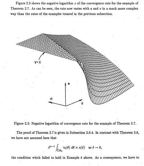
2.6.4 Proof of Theorem 2.7 ... 52
3 C r o ss-V a lid a tio n 59 3.1 Introduction... 59
3.2 Mathematical Models and Cross-Validation in Image A n aly sis... 61
3.2.1 Mathematical Models for the Observations ... 61
3.2.2 The Estimator i ... 63
3.2.3 Two Approaches to Cross-Validation... 64
3.3 R esults... 67
3.3.1 Properties of MSSE and S S E ... 68
3.3.2 Mean Square Results for the Cross-Validation Methods ... 71
3.3.3 Discussion of R esu lts... 73
3.3.4 Uniform a.s. Results for the Naive CV M e th o d ... 74
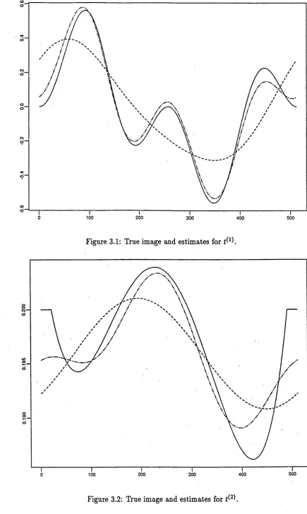
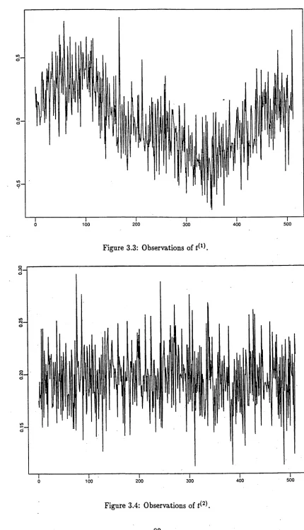
3.3.5 Numerical E x am p les... 77
3.4.1 Some Technical Lemmas 81
3.4.2 Proof of Proposition 3 . 1 ... 89
3.4.3 Proof of Proposition 3 . 4 ... 91
3.4.4 Proof of Theorem 3.5 ... 95
3.4.5 Proof of Theorem 3.6 ... 101
3.4.6 Proof of Proposition 3 . 7 ... 108
3.4.7 Proof of Theorem 3.8 ... 117
3.4.8 Proof of Proposition 3 . 9 ... 127
3.5 Appendix: Rosenthal’s In eq u ality ... 130
4 M ed ian S m o o th in g 133 4.1 Introduction...133
4.2 Image Models and the Median Sm oother...135
4.2.1 Models for the Observations...135
4.2.2 The Median Smoother T ... 137
4.2.3 Approximations to the Median S m o o th e r ...138
4.3 R esults...140
4.3.1 Convergence of T v to T ... 140
4.3.2 The Mean Square Error of the T v ...141
4.3.3 The Mean Square Error of f ...143
4.3.4 Discussion of R esu lts... 144
4.4 P r o o f s ...146
4.4.1 Proof of Proposition 4 . 1 ... 146
4.4.2 Proof of Proposition 4 . 2 ... 148
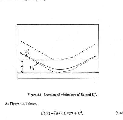
4.4.4 Proof of Theorem 4.4
C h a p ter 1
In tro d u ctio n
This thesis deals with theoretical aspects of some statistical problems which arise in the analysis and processing of images.
In Chapters 2 and 3 we look at blurred and noisy images and consider asymptotically optimal ways of deblurring the observed data. This is followed by proposals of criteria for determining the amount of deblurring needed. The method used for deblurring is partial Fourier inversion and the amount of deblurring required is determined by extensions of the method of cross-validation.
The last chapter explores the non-linear method of local medians as an estimation technique for noise-degraded images, and describes how the window size for the local median must be chosen to provide asymptotically optimal performance.
In these three chapters we present our asymptotic results in the form of rates of convergence of the estimator to the true image with respect to an appropriate distance measure.
1.1
Background and M otivation
Images come in many different shapes and sizes and arise in a large number of areas including science, engineering and medicine. The interpretation of an observed image is not always apparent from the observed data, since the true image has often been degraded in the imaging process, and may therefore only be available in a disguised form.
of analysing and processing images have been developed with the aim of making the observed image more accessible to the human observer.
Many of the common processing techniques such as digitisation, coding, data com pression, image enhancement and restoration, and image segmentation are described in Rosenfeld and Kak (1976). An account of image reconstruction methods, including to mographic techniques, can be found in Chapter 5 of Hall (1979). These methods have been enjoying great popularity in particular in medical imaging. A statistical approach which regards the true images as Markov random fields can be found in Besag (1986).
From the large number of areas within image processing, we are interested in image enhancement and in particular in image restoration. Techniques used in these areas in clude ‘cosmetic’ operations for image enhancement to obtain a subjectively more pleasing image, as well as objective and automatic estimation procedures, whose goal is determi nation of the true image. Image restoration encompasses deblurring and smoothing as well as noise removal, and is applicable to many different types of observed data.
Before we focus our attention on some specific methods, it will be expedient to look at the types of images we shall be concerned with in this thesis. Let T denote the true image and let € denote random noise. Put
Yj = Tj + tj, ( 1.1.1)
for j belonging to some index set in Z d, for d > 1. In this case the true image has been distorted only by the addition of random noise. Examples of observed images of this type are picture transmission or the scanning of images by television cameras (see Section 6.1.4 of Rosenfeld and Kak (1976)).
In many applications, the true image cannot be seen directly, as in (1.1.1), but is transformed in the imaging process, resulting in indirect observations X j given by
X j = f ( T ) j,
for j in some index set. This transformation / may be quite arbitrary, and need not be linear or deterministic. However, in applications it is often reasonable to assume th at / can be approximately described by a combination of a linear operator acting on T and additive noise which is independent of T. We restrict attention to observations of this kind and assume that the linear operator is a convolution operator K. Our observations are then of the form
Xj = K( T) j + €j = (k * T ) j + €j, (1.1.2) where e denotes random noise, ★ denotes convolution, and k denotes the convolution kernel associated with K. In contrast to the observations Yj given by (1.1.1), we shall sometimes refer to the observations Xj of (1.1.2) as indirect observations and to k ★ T
apparatus used in the imaging process. We shall assume that K (or, equivalently, k) is known and deterministic. These assumptions on K do not conflict with reality as the apparatus effect is often known or can be determined accurately. The function k may be regarded as a measure of degradation of the true image, since it describes the blurring or spreading out of the true image. In the engineering literature, k is often called the point spread function or the impulse response (see Section 2.1.1 of Rosenfeld and Kak (1976)).
For images as in (1.1.2), engineers use a wide variety of restoration methods, includ ing inverse filtering, least squares filtering and constrained deconvolution, to name but a few. For descriptions of these and other deblurring methods, see Chapters 6 and 7 of Rosenfeld and Kak (1976). A more mathematical framework for inverse filtering can be found in Twomey (1965). These restoration methods explicitly exploit the fact th at the convolution kernel is known (or can be measured accurately) and can therefore— at least in theory—be removed. Conceptually the simplest method is that of inverse filtering. It also provides a basis for some of the other methods, which address the shortcomings and the arbitrariness of inverse filtering in different ways. In Section 1.3 we describe the technique of inverse filtering, also known as Fourier deconvolution, and point out how it can fail. We then introduce the concepts of smoothing parameter and partial Fourier inversion and show how they can be used as a way of overcoming the instabil ities associated with Fourier deconvolution. The choice of the smoothing param eter is intimately connected with the domain of definition of the Fourier deconvolution. This choice is crucial as it determines the compromise between the smoothness of the esti mate and its faithfulness to the true image. In many practical applications of Fourier deconvolution, the smoothing parameter is chosen in an ad hoc manner or by exploiting specific properties of the underlying physical model. However, because of the trade-off between smoothness and faithfulness of the estimate, or between bias and variance, it is im portant to have a rigorous and objective basis for the selection of the smoothing parameter. We use a specific distance measure as the basis for the selection criterion for the smoothing parameter and then establish the optimality of partial Fourier inversion as a technique for estimating T. This is the topic discussed in Chapter 2. Our results are of an asymptotic nature; we treat a large class of realistic point spread functions si multaneously and allow for correlation in the error, in this way extending previous work in this area (see Hall (1990)).
From the point of view of numerical analysis, the blurred image k ★ T of (1.1.2) is regarded as a Fredholm integral of the first kind, and the problem of recovering T
over a class of functions T of
||X - k * T ||2 -f aA(T), (1.1.3)
where A denotes a regularise^ such as the linearised curvature functional or an entropy functional. (For more details on regularises see Titterington (1985) and Koch and Anderssen (1986).) Although regularisation yields a unique solution, from a statistical point of view this is not enough, since
• the blurred image k ★ T is usually also degraded by the addition of noise as in (1.1.2); and
• the question of how to choose the regularisation or smoothing parameter a is not addressed.
For images as in (1.1.1), cross-validation provides an automatic and objective way of selecting the smoothing parameter. A brief account of cross-validation in nonparametric regression and references to the literature are given in Section 1.4. For indirect images of the form (1.1.2) no analogous method for choosing the smoothing parameter exists as yet, although the problem has been addressed by some authors (see Thompson et al. (1990) and Koch and Tarlowski (1986)). In Chapter 3 of the thesis, we propose generalisations of cross-validation to indirect images X j which exploit the fact that partial Fourier
inversion yields optimal estimates under suitable assumptions. The presence of the blur in the image adds another degree of complexity to the problem of giving a rigorous treatm ent of cross-validation. To make our analysis mathematically more tractable, we therefore restrict the blur to a specific class of point spread functions. This enables us to give precise bounds on the admissible amount of blur in the observed image. Under these conditions on the blur we show that cross-validation performs asymptotically optimally, and cross-validation fails if the blur exceeds these bounds.
estimator than the mean, for example, in the presence of outlier contamination (see Hampel et al. (1986)).
The different areas of research in which medians arise—in the form of running medians or median filters—have developed quite independently so far and little cross-fertilisation exists. In a statistical context, least absolute deviation estimators have been employed in linear regression and time series, for example, and comparison with the mean and some Huber M-estimators exist for various regression models (see Chapter 2 of Bloomfield and Steiger (1983)). In the engineering sciences, on the other hand, median filtering is still very much a practical tool, and despite growing popularity and range of applications, theoretical results are still scarce, and when they exist, are usually of a special rather than a general nature. This may be due to the sentiment expressed by Huang (1981) that a ‘theoretical analysis of median filters is very difficult’, which precedes papers by Tyan on deterministic properties of median filters and by Justusson on properties of median filters applied to pure noise.
The great appeal of median filters in the engineering sciences combined with the lack of a theoretical foundation has motivated us to look at median filters or median smoothers from a more theoretical and statistical point of view in Chapter 4. Unlike Justusson (see Huang (1981)), who considers pure noise, we are interested in non-constant images which are degraded by noise and consider observations of the form (1.1.1). For such data we derive an expression for the asymptotic rate of convergence of mean square error of the median smoother as the sample size increases. From this expression we deduce the asymptotically optimal window size and the corresponding rate of convergence. To prove our results we use the framework of M-estimators and robust statistics, which is briefly described in Section 1.5. Our analysis also shows how the rate of convergence depends on the dimension d of the observations, and it may be rather unexpected to observe that the rate depends on d in different functional forms depending on whether d is less than or greater than four.
1.2
N o ta tio n a l P relim inaries
In this section we summarize notation that may not be standard.
N orm s and the inner product. For x = ( x i ,. . . , Xd)T € Rd, we use the following norms:
d
1*1 = ]C l*il
oo = sup |x,'|.
Sometimes we shall also write ||x||i for |x| and ||x| | 2 for ||x||. For vectors x, y G Rd,
the inner product of x and y is
d
ix ,V) = ^ 2 xiVi-t=l
Spaces o f functions. Our images and point spread functions may belong to the fol
lowing spaces:
= {/ : R d-< t :
J
|/ | p < 00} p = l,2L"(RJ,R) = :
J
\ f \ ” < 00} p = l,2=
{ / :
- C : £ l/(*)lP < °°} P=M
ke7Ld
C “(Rd) = { / : Rd —► ([ : f is a times continuously differentiable} C°°(Rd) = { f : R d —»C : / is infinitely often differentiable}.
Functional relationships. Let f and g denote positive real-valued functions defined
on R d. We write
f ~ 9
if there exists constants c\ and C2 > 0 such that ci<7(x) < /( x ) < C2<jr(x) for all x 6 R d;
and
/(x ) x g(x) as x —►xq
if f ( x ) / g ( x ) and g ( x ) / f ( x ) are bounded as x —►
xo-Let an and 6n, n = 1 , 2 ,..., denote sequences of positive real numbers. We write
an = 0( bn)
if there exists a constant c > 0 such that an/bn < c as n —*• oo. We write
fln = o(6n)
if an/bn —► 0 as n —► oo; and
dn ~ bn
if an/bn —► 1 as n —► oo.
1.3
Fourier Inversion T echniques
Fourier transforms apply to both discretely and continuously defined functions, and we consider both cases simultaneously in this section.
1.3.1
D efinitions and Properties of Fourier Transforms
Let X denote a blurred image B degraded by additive random noise e, so
X = B + e. (1.3.1)
Here X , 5 , e and T (below) either all denote functions defined on Rd or all denote functions defined on 7Ld. We assume that
B = H * T , (1.3.2)
where T denotes the true image, H denotes the blur or point spread function and ★ denotes the convolution product, which is defined in the following way. For F , G € £ l ( R d) ,
( F * G) ( x ) = / d F(y)G(x - y) dy for x € R*; (1.3.3)
J w \
and for / , g € t l {7Ld),
( f * 9 ) { j ) = ^ f ( k )g(k - i ) for j € H.d• (1.3.4)
ke7Ld
For indirect observations of the form (1.3.2) with known function H, Fourier decon volution represents a natural way of recovering T from B. The method described in Subsection 1.3.2 works for discretely as well as continuously defined functions; the choice of the appropriate Fourier transform is the main distinguishing feature. For F € X1(Rd), the d-dimensional Fourier transform, <f> of F is given for 9 € by
4>{9)
=f
d F(x)e*'<x’*> dx,
(1.3.5)
JRand if € i 1(R'i), the inverse Fourier transform of is defined for x € R'‘ by
4>(x)
= (2x)-J
f
d <f>(6)e- il'x'e'1 de.
(1.3.6)
JR
Sometimes it will be convenient to write <j> = FT( F) and <j> = I F T (</>).
inverse Fourier transform <j> (if it exists) are given by
m =
YfUVm > oel-*,’
r]d
}<=ZlJ
4U) = ( 2 v ) - d
f
W ) e - W l d 0 , j € 7LJ. (1.3.7)^ [ - 7 r , 7 r ] d
It is usually clear from the context which Fourier transform is appropriate, and we shall therefore often omit the word discrete.
For notational simplicity we shall describe the properties of Fourier transforms and the method of partial Fourier inversion in terms of functions F, G £ X1(Rd). The analogous properties of the discrete case can easily be derived from this and are therefore not usually given. For details on d-dimensional transforms and the results quoted below, see Vo-Khac Khoan (1972).
A . T he Inversion T heorem . If F 6 L l ( Rd) and </> = F T ( F ) 6 T1(R<i) and if
<j>(x) = ( 2 x ) - d
f
ä d0 for x € RJ ,J R then <j> is continuous and
F(x) = 4>(x) a.e.
B. C onversion o f convolutions to pointw ise products. Let F , G 6 T1(Rd), and
let (f> and 7 be their respective Fourier transforms. If H denotes the convolution of F
and G and x denotes its Fourier transform, then
XW = <t>Wl{0) for 0 e Rd. (1.3.8)
The next result constitutes one of the main theorems of Fourier transforms for L
2-functions. We shall make use of it repeatedly in Chapters 2 and 3 and therefore quote it for L 2( Rd) as well as for t 2(7Ld).
C . Parseval’s identity. If F, G £ L2(Rd), with Fourier transforms $ and T, and / ,
g £ £2(7Ld), with Fourier transforms 4> and 7 , then
j Rd F( x)G(z) dx
(2x)-dJ ^ m m de,
1 .3 .2 F ou rier D e co n v o lu tio n
As we have seen in result B above, the Fourier transform interchanges convolution and pointwise product. This property of Fourier transforms is the key to Fourier filtering and Fourier deconvolution. We now turn to the blurred image B of (1.3.2).
Let r , x and ß denote the Fourier transforms of T, H and £ , respectively. Assume that x($) 7^ 0 for 0 £ Rd. Fourier deconvolution of B by \ is the process which results in the function f given by
f(x ) = /FT(/3X- 1)(x) = (2 * )-J J ^ A ß W / x m e - ^ d9. (1.3.10)
Because of its special role in Fourier deconvolution, the Fourier transform \ of the point spread function is called the Fourier kernel. In the engineering sciences, x is often called a transfer function (see p212 of Rosenfeld and Kak (1976)); it may also be called a characteristic function if H is a probability density.
The inversion theorem A and (1.3.10) together show that T can be reconstructed a.e. from
i?,
providedx(#)
i1
0-
Problems arise however ifx($) =
0 for some 9£
Rd. Sinceß = x r, ß = 0 whenever x = 0 and this leads to indeterminate ratios in the integrand of (1.3.10). Thus, even in the absence of noise, it is in general not possible to reconstruct T
from B exactly. The situation is exacerbated for observations X which contain random noise €. If £ and u denote the Fourier transforms of X and e respectively, then the zeroes of £ and v will not usually coincide. As a consequence, u / x would be very much larger than t in neighbourhoods of the zeroes of
x-The problem of zeroes of x in the deconvolution step can be overcome if one restricts the division by x and the subsequent Fourier inversion to a subset of R d on which x is not too close to zero. This is the approach we adopt and now describe briefly.
Assume th at H £ X1(R(i). Let 0 be a subset of Rd on which x -1 is defined and bounded. For observations X = H ★ T + e, the partial Fourier inversion estimator T with smoothing set 0 is defined by
T( x) = (2* )~J J@{m/x(0)}e-(1.3.11)
The set 0 is also called the inversion set. Sometimes we want to emphasise which smoothing set is used in the definition of T. In this case we write T© instead of T.
Often, the smoothing set will depend on a parameter, as in the following examples, which illustrate the main types of smoothing sets we shall employ.
For 6 > 0, put
This choice of smoothing set is appropriate if x($) —► 0 as 9 —► oo. In this case, Os
eliminates the high frequencies. These contribute very little in the case of smooth images T, and thus not much information is lost in employing 05 instead of Rd.
For functions x with isolated zeroes at 0,- € i = 1 , 2 , . . a possible choice for Os
is given by the following: Fix ö > 0, and put
$5 = {ip £ Rd : ||ip — 0,|| < 6 for some i}
06 = Rd \ « s. (1.3.13)
Judicious choice of the inversion set 05 is important as it provides a compromise between faithfulness of the estimator T to T and roughness of T. As Os / or as
6 —► 0 in (1.3.12)), T —►T + I F T ( v \ ~ l), and therefore T becomes less smooth as more frequency components are included in the inversion set. A smoother estimator T is obtained by selecting a smaller inversion set 05 (e.g. by choosing a bigger value for the cut-off point 6); the noise component of T will be more smoothed out, while the image component of T becomes a worse approximation to T. Because of its role in the choice of the set 0 5, 6 is often called the smoothing parameter, in analogy with smoothing parameters in statistical curve estimation.
The method of partial Fourier inversion has been used for a number of decades, especially in the engineering sciences where it is often referred to as Fourier filtering. In numerical analysis, on the other hand, the method is often described as numerical filtering (see for example Phillips (1962) and Twomey (1965)). Other authors (e.g. Hall (1987a), Titterington (1985)) call the estimator T of (1.3.11) a regularised estimator and associate zero weights with the set Rd \ Os, and unit weights with 0 5. Practical implementations of Fourier deconvolution are described in Rosenfeld and Kak (1976) and in Koch and Tarlowski (1987).
1.4
C ross-V alidation in N on p aram etric R egression
1.4.1 P erfo rm a n ce M ea su res and R a te s o f C o n v erg en ce
Let Yj denote data observed at points xj, j = 1 , . . . , n such that
Yj = m( xj ) + ej, (1.4.1)
approxima-tion one usually considers pointwise or global distance measures. A common pointwise measure of accuracy is the mean square error, MSE, calculated at a fixed point x:
MSE(x) = E{rh(x) - m ( x ) } 2. (1.4.2)
Sometimes global measures are preferable, since arguments that have been developed in the more general framework of global convergence also apply to problems of pointwise convergence. The following quadratic measures are often used:
SSE = ^2{rh( xj ) - m ( x j ) } 2
j =i
MSSE = E(SSE). (1.4.3)
In some cases, weights are part of the definition of SSE and MSSE. The measure SSE is called sum of squared error or loss and MSSE is called mean sum of squared error or risk (see p l6 of Eubank (1988)). Many other choices of distance measure are available, such as the absolute and the maximum deviation of in and m, but we shall not be concerned with those. In Chapter 3 we shall use the global measures SSE and MSSE to assess the performance of cross-validation, while the simpler measure MSE of (1.4.2) will suffice when we consider the performance of partial Fourier inversion estimators in Chapter 2 and of median smoothers in Chapter 4.
In many situations one wants to assess the performance of an estimator as the sample size increases and to determine its rate of convergence to the true function m. Consider functions / , g : N —►R + which converge to zero as n —> oo. We say / and g have the
same rate of convergence if there exists a constant c > 0 such that / ~ eg.
Let d denote a distance measure and assume that d depends on the sample size n of the data (e.g. d =SSE or d =MSSE). Let m = fh(n) denote an estimator of m. We say that a function r : R+ —►R + is an optimal rate of convergence with respect to d if there exist constants ci, C2 > 0 such that, as n —► oo,
d{m(n), m} < c\ r{n)
_inf d { m( n ) , m} > C2r(n), (1-4.4)
m (n)
where the infimum is taken over all possible estimators for m. An estimator m of m is called optimal with respect to d if it satisfies the first of the two conditions (1.4.4).
1.4.2
Choice of Smoothing M ethod
In practical applications of smoothing data one encounters two types of problems:
• the choice of the smoothing method; • the choice of the smoothing parameter.
The selection of the smoothing method depends on a variety of factors, and different methods apply to regression data Yj and indirect observations X j of the form (1.1.2). For this reason, we shall only briefly review some of the methods used in nonparametric regression. As far as the second problem is concerned, the method of cross-validation for selecting the smoothing parameter will be described in Subsection 1.4.3, and it is this method which we shall generalise and adapt to the requirements of indirect observations
X j in Chapter 3.
In the context of nonparametric regression, the commonly used methods include local averaging, kernel smoothing and spline smoothing. In many of these methods, the estimator m of m can be expressed as
rh(x) = ^2ct j(x)Yj (1.4.5)
for suitably chosen weights Qj(z). For kernel smoothing methods, Priestley and Chao (1972) were amongst the first to suggest the use of weights which are derived from densities and which can be parametrised by a scale parameter h. This parameter adjusts the size of the weights and is often called the bandwidth of the kernel weights. Typically one has weights ctj(x) given by
OLj(x) = Kh(x - Xj )/ fh(x), (1.4.6)
where
n
fh(x) = n~l J 2 Kh(x - Xj) j=
i
Kh(u
) =
h~1K(u/h).(
1-
4-
7)
For details see Chapter 3 of Härdle (1989) and references therein.
In contrast to kernel smoothing, in the method of spline smoothing the estimator m of m is taken to be the minimiser of S \ over a class of admissible functions ra, where
S\(fh) =
y^{r
7
-
fh(xj)}2
+
AJ
{m^^(x)}2 dx, i = 0 ,1 ,2 ,— (1.4.8)m(*) denotes the ith derivative of ra, and A > 0. A comparison of (1.4.8) and (1.1.3) shows that spline smoothing is a special case of regnlarisation. The most common form of Sx is that in which i = 2 in (1.4.8). For this case, Schoenberg (1964) and Reinsch (1967) have shown that if the class of admissible functions consists of all functions with square integrable second derivatives, then for each A > 0, S \ has a unique minimiser, which is a cubic spline. Furthermore, the minimiser of S \ is of the form (1.4.5). A nice account of spline smoothing can be found in Wahba (1990).
The smoothing methods mentioned so far are distinguished by the existence of a well-developed theory and a wide range of applicability. Other smoothing techniques may be preferable under certain circumstances. For example, if one wanted an estimator which is resistant against outliers and is capable of modelling discontinuities, median smoothing would be more appropriate. In connection with blurred and noisy data X j = (k*T)j+€j (see (1.1.2)), yet another smoothing method, namely partial Fourier inversion, is appropriate for finding an estimator T of T. Common to all these methods, however, is the dependence of the estimator on a smoothing parameter.
1 .4 .3 S e le c tio n o f th e S m o o th in g P a r a m e te r by C r o ss-V a lid a tio n
We assume that the distance measure SSE has been chosen to assess the performance of the estimator ra. The estimator in depends on a smoothing parameter h, which we indicate in this subsection by writing ra^. The aim now is to choose h in such a way that
ihh, minimises the order of SSE. Such a choice of h will be called optimal with respect to SSE. Let h denote the optimal smoothing parameter. Then
(1.4.9)
since the term 23 m( x j ) 2 does not depend on h. This definition of the optimal h is useful for a theoretical analysis. However, in practice this approach cannot be used, since SSE cannot be computed without a knowledge of m itself. Closer inspection of (1.4.9) reveals that the term 23 ^ ( ^ j ) 2 can be estimated from the data but the cross-term 23 fn^(xj)m (xj) cannot. Since one cannot calculate this term from the data, the idea is to estimate it. A naive estimate would be '$2™’h{xj)Y j, where m ( x j) has been replaced by Yj. This procedure, however leads to a biased estimate of SSE (see Section 5.1 of Härdle (1989)), and is therefore not recommended.
Amongst the possible methods of finding an unbiased estimate of SSE, we concentrate on the leave-one-out or cross-validation technique (for some other methods see Section 5
h — arg min SSE(h)
h
= a r g m in ^ { m /l(xj) - m( x j ) } : j=l
= arg min <Y]rhh{xj )2 - 2
Y]
m h{xj )m(xj ) > ,of Härdle (1989)). The basic idea of cross-validation is the following:
• For each j = 1 , . . . , n, divide the data into two uncorrelated parts such as Yj and
{Yl , Y 2, . . . , Y j . u Y1+1, . . . , Y n}.
• Use one part to assess the performance of an estimator defined on the other.
For this leave-one-out method, one would estimate m ( x j ) by fh(xj) = Yj and then compute an approximation rh\(xj) of rhh(xj) from {Yjt : k / j } . Thus
R = i t ™h(x j ) 2 ™Uxi)™(xi)
j=l j=i
(1.4.10)
would be an estimate for
n n
R = Y ^ ™hixj ) 2 - 2 5Z rhh(xj ) m(x j ).
j=i j=i
(1.4.11)
In fact, cross-validation is a technique for selecting the smoothing parameter which is mathematically justified because one can show that under appropriate conditions the minimiser h of R satisfies
R(h) !
inf h R(h) a'S' (1.4.12)
A proof of this for nonparametric regression can be found in Vieu (1991) and an earlier result, showing convergence in probability, is proved in Härdle and Marron (1985). For rates of convergence of h to h, see Härdle et al. (1988). For density estimation, an analogous result goes back to Stone (1984).
One of the features of cross-validation used in proving results of this kind is the fact th at the cross-terms in fh\{xj)fh(xj) are calculated from uncorrelated parts of the data and the cross-term in R has therefore zero expectation. This observation is an important consideration in our development of cross-validation for blurred data in Chapter 3.
1.5
M -E stim a tio n
For independent observations Z i , . . . , Z n from a distribution with density fo, 6 an un known parameter, the maximum likelihood estimation strategy is to maximise the like lihood function, or equivalently, to minimise (over 9)
- y > g
MZi ).
(i.5.i)
The minimiser 9 of (1.5.1) is called the maximum likelihood estimator of 0. For the estimation of the parameter in a location family (for which fe(z) = f ( z — 9)), the idea of maximum likelihood estimation was generalised in Huber (1964) by allowing a larger class of functions in the definition (1.5.1). The resulting estimator is called an M-estimator, and is defined by
n
9 = arg min />( Zt- — 9), (1.5.2)
6 * = i
where p denotes a ‘distance-like’ function. The interest in a generalisation of maximum likelihood estimation was motivated by a desire to bound the influence of extreme or outlying observations, while at the same time maintaining acceptable efficiency when outliers are not present.
Often, the function p is differentiable and 9 is then a root of the equation
n
2 > ( Z i - f l ) = 0, (1.5.3)
« = 1
where ip(z) = p'(z). If p(z) = z2, for example, solution of (1.5.3) leads to 9 = Z, the sample mean. As well as the mean, there are many other useful M-estimators which can be determined by choosing ip in (1.5.3) (see pl03ff of Hampel (1986)). In cases more complex than the mean, (1.5.3) must be solved numerically. Numerical methods for solving equations often rely on the existence of the derivative, and, similarly, theoretical properties of the estimator are also often derived under the assumption that ip has a derivative.
T he m edian is an M -estim ator w ith p(z) = \z\. The function ip as in (1.5.3) exists for th e m edian, namely, ip(z) = sign(^), and th e m edian is a root of (1.5.3), which can be found explicitly. However, because of the non-differentiability of this ip, theoretical properties of th e m edian are more difficult to obtain.
C h ap ter 2
P a rtial Fourier Inversion
2.1
In trod u ction
Most theoretical analyses of indirect images are confined to discrete observation points. This clearly reflects the practical set-up: data are recorded at discrete points in time or space. For the latter, lattices based on squares or rectangles are mostly employed, but some imaging devices such as texture analysers (see Serra (1982)) also use triangular and hexagonal lattices.
For a theoretical study of images, however, the discrete n atu re of th e recorded d a ta corresponds to modelling the sampling distribution, i.e. th e point spread function, by a discrete distribution. This imposes severe lim itations on the class of distributions th a t can be treated (see Hall (1990)), and excludes interesting and realistic distributions,such as those treated below.
For this reason, the analysis presented here is based on continuously defined obser vations. This situation may be regarded as the limiting case of discretely observed data when the pixel size or the separation between observation points tends to zero. Typically we shall assume that X is observed at points in a convex subset 1Z of JRd. This will allow us to treat a large class of problems simultaneously, including the out-of-focus blur and the motion blur of Hall (1990).
In the models discussed in this chapter, we shall always assume that the point spread function is known. This corresponds to knowing (or measuring) the effect of the imaging apparatus, and is common practice in many applications in engineering.
All our observations are of the form
where ★ denotes convolution, T denotes the true image, H the known point spread func tion and N denotes random noise. We examine the method of partial Fourier inversion and show that it provides an optimal method for image enhancement for a widp rancro
of images and point spread functions. Fourier inversion techniques and, in p articu lar, the W iener filter are regarded as standard tools in th e engineering sciences. We concentrate on determ inistic images, while the W iener filter approach assumes th e images to be weakly statio n ary random fields. For this reason the W iener filter does not apply to the situation considered here.
In Hall (1987a, 1987b) motion blur and out-of-focus blur were applied to piece-wise constant images or test-patterns and the performance of restoration methods was considered from the viewpoint of consistency. Somewhat later, in Hall (1990), the same point spread functions were used to degrade images which may be regarded as discreti sations of continuously differentiable functions, and precise upper and lower bounds for the mean square error were calculated. The results presented here extend those of Hall (1990) in several important aspects:
• By considering continuously defined image models a wide range of realistic point spread functions can be treated in a systematic way.
• Dependent noise models are developed which replace the assumption of white noise treated in Hall (1990). Although much simpler to deal with, the white noise model is les*3 g e n e ra l.
An abridged version of the results described here is given in Hall and Koch (1990). In the next section we describe the class of images and point spread functions that will be considered. Section 2.3 is concerned with models for correlated noise, and consid ers moving average noise, which may be taken as a concrete example of the kind of noise we are dealing with. In Section 2.4 we describe our results, in particular our main result, Theorem 2.6, which shows that under suitable regularity conditions, partial Fourier in version is an optimal reconstruction method in a mean square sense. Section 2.5 contains some simple examples which demonstrate the scope of our theorem. Furthermore, we look at some applications which give specific rates of convergence for the partial Fourier inversion estimator. Proofs of the results of Sections 2.4 and 2.5 appear in Section 2.6.
2.2
M od els for Im ages and Im age D eg ra d a tio n
2 .2 .1 Im a g e M o d els
We assume that the true images T are real-valued functions, defined on Rd (d 6 N,
d > 1), which are absolutely integrable. These properties of T we summarise by writing T 6 L l ( Rd,fV). The integrability of T guarantees the existence of a continuous and bounded Fourier transform r of T. In fact, it is convenient to describe classes of images in terms of their Fourier transforms in the following way.
. (j e t c j 0 ) =
For tq 6 Z/(R , R+), To symmetnc^define the image class C(tq) by
C(t0) = { T € L \ K d, R) : |r(0)| < r0 V0 € Rd} (2.2.1)
and call To the envelope of the class of images C(to). Thus To is an envelope if To G L l ( Rd,
R+),
To is symmetric and To defines a class of images in L l ( Rd,R).
Let To denote the inverse Fourier transform of r0. If To£ X1(Rd, R),
then To G C(t0).In this chapter, To will always denote an envelope of a class of images. From (2.2.1) it follows th a t the class of images C(t0) is com pletely characterised by properties of r 0. Of particular interest here will be those envelopes t0 of polynomial
decay and of exponential decay, described next. Locally, images of this type may be regarded as approxim ations to realistic images such as extended brightness sources in astronom ical imaging.
A . Im ages w ith poly normally decreasing Fourier transform s. Assume that
there exist A > 0, a > 0 such that
to(0) = A(1 + 11011)-° for €
Rd.
(2.2.2) Equation (2.2.2) implies that supö{ro(0)||0||“} < oo. If furthermore M kro € L x(Rd), fork < a, where ( M kro)(d) = 0kTQ(0), then
C(r0)
= { T e
i '( R d,R) : |r(0)| < A(1 + ||0 ||) - V0 6 Rd>
corresponds to the set of true images which are a times continuously differentiable, that is, C(t0) C
Ca(Rd)
(see p.26 theoreme of Vo-Khac Khoan (1972)). Here the parameter a indicates the smoothness class of the images. The higher the value of a, the smoother the images are. Images of this kind are used in Examples 1 and 3 of Subsection 2.5.1.B . Images w ith exponentially decreasing Fourier transform s. For constants
A > 0, a > 0, define t0 by
This type of image is used in Examples 2 and 4 of Subsection 2.5.1. Of special interest are the cases p = 1,2, which we now consider.
If p = 2, then ro(0) = A [ ] t i exp( —a | 1 2), and To = /T T ( r 0) is given by
T0(x) = A e x p (-||x ||2/4a) for x G R d. (2.2.4)
The class C(tq) then is a subset of R), the class of infinitely often differentiable functions from to R:
C(r0) = {T G C °°(R ^R ) : |T(x)| < A e x p (-||x ||2/4a) Vx G Rd}.
If p = 1, then To = I F T ( r 0) is given by
d
To(x) = A J J { 2 a /(x 2 + a2)} for x G Rd, (2.2.5)
t=i
and C(to) corresponds to the set of images which are proportional to products of Cauchy distributions (see also paragraph A of Subsection 2.2.2 below).
We could easily treat more general classes of images than those given in paragraphs A and B above, such as combinations of (2.2.2) and (2.2.3) or images with envelopes ro of the form to(6) = A( l + ||0||)-O{1 + max(0,log ||0||)}~6, A, a,b > 0. For reasons of clarity and simplicity, the examples given in later sections will concentrate on images of the classes described above .
2 .2 .2 M o d e ls for th e B lu r
In our model, the true image cannot be observed directly, but is degraded in a linear and systematic way by a deterministic function. This function is assumed to be known and will be denoted by H throughout this chapter. It is called the blur or the point spread function; its Fourier transform \ is called the Fourier kernel.
We assume that
H : Rd —► R is symmetric, and
J
H(x) dx = 1.The assumption f H = 1 allows us to regard H as a density, and its Fourier transform X as a characteristic function, as will be convenient in paragraph A below.
The blurred image, denoted by B, is of the form
This image would be observed in the absence of random noise.
A. Point spread functions with thin tails. We are interested in point spread
functions H which are concentrated near the origin, that is, point spread functions with compact support or with “thin” tails .
Polynom ially decreasing kernels: For a > 0, define \ by
x W = c( 1 + ||0||)"a for 9 £ Rd, (2.2.6)
where c > 0 is chosen such that x € L l (Rd) and f H( x) dx = 1. If M °x 6 L l {Rd), where
( M ax)(0) = 0ax{0) f°r 0 € then H is an a times continuously differentiable function. (See also paragraph A of Subsection 2.2.1 and Examples 1 and 4 in Subsection 2.5.1.)
Exponentially decreasing kernels: For c > 0, a > 0 define x by
X(0) = exp(-c||0||a ) for 9 £ R d. (2.2.7)
Fourier kernels of this kind are also used in Examples 2 and 3 in Subsection 2.5.1. amd d - 2 ..
Of particular practical interest is the case a = I\ Fourier kernels of this kind appear, for example, in remote sensing problems. For a = 1 the blur function H becomes
H( x) occ[}jx||~ ■+ c*~] for oc e (2.2.8) which may be interpreted as the filter corresponding to downward continuation by dis tance c in the magnetic field equation (see Koch and Tarlowski (1987)).
Characteristic functions o f stable distributions: For 0 < a < 2, c > 0, define X by:
d
X(9) = e x p ( - c ^ |0j|°) for 9 £ Rd. (2.2.9)
t = i
The corresponding point spread function H is given by
H( x) = {2Tr)~d
I
ex p (-c |0 j|a ) exip(-i9jXj) d9j for x £ Rd. (2.2.10)j=i
The point spread function H given in (2.2.10) is a symmetric function which has derivatives of all orders for x E R d. Expressions for H for a = 1 and a = 2 were given
in (2.2.5) and (2.2.4) respectively. For a = 2, the Fourier kernel x(#) = exp(—c||0||2) is also a special case of (2.2.7). A further description of the densities of stable distributions for a / 1, a ^ 2 can be found in Ibragimov and Linnik (1971), Theorem 2.3.1, p48.
B. Point spread functions with com pact support. We describe two kinds of point
spread functions here: products and convolution products of functions with compact support.
Products: For v E N, v > 1, define H u on Rd by:
H (x) = I
CiMn?=i{cos(7r:rt/2 )} 1'- 1 if x , E [ - l , + l ]o if x, e R \ [ -i, +i],
(2.2.11)
where Ci(v) = {cos(7rx/2)}l/ 1 dx , so f H = 1
For v = d = 1, Hi is just motion blur. As v increases, H u becomes smoother near 1, and more concentrated near 0, becoming the d-dimensional Dirac delta-function in the limit.
The Fourier kernel \ u on Rd is given by
x ,W = {2> - v - Ir (t/)}dc,(</)
X n s in ( 9 , - ^ * ) r (
J
{ r (I
+ . (2.2.12)This follows from Lemma 2.6.2, which is proved in Subsection 2.6.4. This lemma also gives the zeroes of \ u for the case d = 1, which occur at 0 = ± ( v — 1)t/ 2 + t i t, n >
1. Since \ u is the d-dimensional product of the one-dimensional version, \ u = 0 on hyperplanes N„ given by
Afv = {0 = (0,) : 0, = ±(v — 1)tt/ 2 -f tit, n > 1 for some i = 1 , . . . , d}
Furthermore, as
ix,wi
xn
:= 1
sin(0, — ( i + M ) "»
Convolution products: Let II denote the rectangular function in Rd defined by
nix)=i 2~i
* e [ -
1.+i]-1 0 a; € Rd \ [ - l , + l ] d.
For v 6 N, v > 1, let Hu denote the //-fold convolution product of II:
Hu(x) = ci(u) n (x ), (2.2.13)
where C\(u) is chosen so that f Hv = 1.
As in the case of (2.2.8), for v = d = 1, H\ is motion blur, and for v — 2, H v is the product of triangles with support [—2,2]. As v increases, H u becomes smoother, and its support increases.
If IIi denotes the rectangular function on [—1,1] of height 1/2, whose Fourier trans form is 9~l sin#, then II(x) = nf= i IIi(xt), and thus the Fourier kernel \u of H v becomes
^ ) = ' > M n ( n x ) =ciWn ( x ) ^ $ € *d-
(2-2-14)
As in the previous example, \ v = 0 ° n hyperplanes Af where
Af = {0 = ( = nir, n € 2Z for some i = 1
and, asymptotically, \ u decreases polynomially:
d
Xu{0) ~ + \ei\)~l/ a s \W\ ° °
-t'=l
2.3
M odels for C orrelated N oise
The random degradation in the observations is modelled by an additive random field
N : Rd —► R. As we are deviating from the white noise model, it will be convenient to characterise properties of the noise process N in terms of the autocovariance function 7W of N defined by
7n(x,v) = E [{7V(x) - E N ( x ) } { N ( y ) ~ EJV(y)}] fo r ^ t/G R '* . (2.3.1)
The process N is (second order) stationary if its autocorrelation function 7^ satisfies
If satisfies (2.3.2), it can easily be seen that 7 ^ depends only on the difference x — y,
and may therefore be regarded as a function 7 ^ : Rd —>► R, as is done from now on. Condition (2.3.2) is sometimes called weak stationarity or covariance stationarity. As a consequence of (2.3.2), 7jv is symmetric, 7jv(0) > 0, and 7 ^ attains its maximum at
x = 0. (For further properties of 7# see p i Iff of Brockwell and Davis (1987).) Assume that the random field N : Rd —► R satisfies
N l EN = 0, EN 2 = 1;
N2 N is (second order) stationary; N 3 1N 6 i 1(R‘i).
The last property of N guarantees the existence of the Fourier transform fw of 7# , called the spectral density, which is defined by
f N(0) =
j
d 7w( i) e i<I 'e> dx for 0 € R^. (2.3.3)The bounds on the mean square error discussed in the next section depend on the noise solely via its spectral density.
For the remainder of this chapter, N will always denote a second order stationary random field, satisfying N l —N3.
Let 7n = {7tv,* : t > 0} denote a family of autocovariance functions for N. The value of t governs the amount of dependence or the range of dependence of the noise process
N: we assume that the dependence between N( x ) and N( y) decreases as t decreases.
As an illustration, let 7 ^ denote the autocovariance function of N and define the family {7N,t] by:
W ( I ) = W (X ), I for x € RJ , t > 0.
7
N,t(x ) =7
n
(<
*x)J
As t —* 0, 7w,* tends to zero more quickly. It follows that the correlation between N ( x) and N( y) diminishes more rapidly too.
A family of autocovariance functions { 7 gives rise to a corresponding family of spectral densities {fN,t} yia the Fourier transform relationship (2.3.3). If jN,t is defined by (2.3.4), then /)v,t satisfies:
/am(0)
f N , t W
/n(0) }
We are now in a position to state further properties of the noise process that will be required in Theorem 2.6. Let /y v = { /at,*} denote a family of spectral densities of N such that
N 4 |/yv,*(0)| < c \td for 9 £ Rd;
N5 inf||0||<C2t-i fN,t(0) ^ c3^ for 9 € Rd;
for constants C2, C3 > 0, where C2 may depend on C3.
It is easy to check that the family {/yv,*} given by (2.3.5) satisfies N 5, if /yv is bounded away from zero in a neighourhood of 9 = 0, since
inf
l l « l l < C 2 * - 1fN,t(<>) =
inf tdfiv(t9).
Note th at /yv is bounded, being the Fourier transform of 7yv, and thus N 4 holds.
For the remainder of this section we look at a specific example of a correlated noise process which satisfies N I —N5.
Let W denote a d-dimensional Wiener process or Brownian sheet, th at is, a Gaussian process defined on R+ with mean zero and covariance structure
d
E{W(*)W(#)> = XI(x; A »■•). (2.3.6)
t = l
where u A v = min(u,u). For more details on Wiener processes see Adler (1981). For / > 0, put Ai = [0,/]*, and define N : Rd —► R by
N( x ) = J ^ d b(u) dW (x — u), (2.3.7)
where b(x) = / d!2 if x £ A/ and 6(x) = 0 otherwise, and IF is a Wiener process as in (2.3.6).
Proposition 2.1 Assume that N satisfies (2.3.7). Then N is an MA(l)-process with
spectral density /yv given by d
f N(0) = ld I J sin2(/0t/2 )/(/0 t/2 )2 for 6 £ Rd (2.3.8)
t = i
which satisfiesN I —N5.
P ro o f o f Proposition 2.1
IX of Doob th a t N is a random process such th a t EN = 0. By Section 8 C h ap ter XI of Doob,
N
m ay be regarded as a moving average process, and is therefore stationary. A change of variable now allows us to rew rite N in the following form:N( x) = l X b{x - u ) dW{u), (2.3.9)
Jx-lj
where j = ( 1 ,1 ,..., 1)T G E d. Now, for x, r G Rd, ^ (t)5* E iNte+'ONUXj is giue*
rx-\-T rx
E{ N( x + t) N (x)} = / b(x + t - u)b(x - v) E{ dW( u) dW( v) }
J x + T - l j J x - l j
rx+T rx
= / b(x + r — u)b(x — v)6(u — v) dudv.
Jx +T — lj J x — lj
Here 6 denotes the Dirac delta-function in d dimensions, and
6(u — v)dudv = E { dW (u)dW (v)},
which follows from (2.3.6). Next observe that f f 6(u — v) dudv = f dv, and thus
E{iV(x + t) N(x)} = j b(x + r — v)b(x — v) dv
J x - i j
= / b(v — r)b(v) dv Ja,
I l~d n t l ( ' - N ) for r e A,
I 0 for Ai.
This shows that N is second order stationary. Thus we may write
7
n(t)= E
{ N( x+
r ) N( x ) }= /
d£[(/ - M)!^
(2.3.10)where Xa, denotes the indicator function of A/. If r = 0, 7n(0) = 1 by (2.3.10), showing that N has unit variance for each x G R d. Clearly, 7at G X1(R<i).
Since N is stationary and IT is a Gaussian process, (2.3.7) defines a d-dimensional MA(/)-process.
It remains to show (2.3.8), N 4 and N5. Here we use the fact that f u , the spectral density, can be written as the d-fold product of one-dimensional Fourier transforms. For 9 G Rd,
/ N{9) = J Rd~tN(x)e'(x'6) dx (by (2.3.3)) r d
—
Z
/TT(Z—
|xt|)exp(iE xtA ) dxJ a ‘
i
i= l - d f[ {si n(Wx/ 2)/ (9t/ 2 ) r
i= 1 d
= /<fn { s in (^ 7 2 )/(W ,/2 )} 2. (2.3.11)
InSevT -£.*10 p Iv
-Tq(x) = (27r)-d [ r ( ö ) e - i(l',’> d$ Jo
k6 {x) = (2ir)-d d6. (2.4.3)
T he lim it (2.4.2) exists under th e assum ptions th a t N has continuous sam ple paths and th a t x -12© £ T1(Rd). To see this, note th a t
T*{ x) = (2*)~J f f ( H * T ) ( y ) I K(!/)x (Ö )-1I e ( ö ) e - (''- I '4> dyd6
Jo JR
+ (2x ) - d / f N ( y ) x ( e ) ~ 1e - ^ - x'e> dydß
Jo Jn
For th e determ inistic p art of Tr,th e integrand is dom inated by
Sl(y>Ö) = |(H*T)(y)x (ö)-
1
I
0
(e)|,
and gi G L1(R d x Rd) by Problem 1, pl0 6 of D udley (1989). The D om inated Convergence Theorem therefore applies to yield
- • hr- V
lim f IDj( Ä * T ) ( y ) I Ä(y )X(Ö)-lI e (ö )e -i<’' - ^ dydO tctR Jo JR
=
& * ) - * [ I. l i m f K * T ) ( y ) I K(y)x(ö)-
1
X
0
(Ö)e-<!' - ^
Jo JR ^TlR
= ( 2 i ) - d / r ( e ) e ’<1>9> dfl = T0(x). (2.4.4) Jo
Let ranft denote the random p art of Tr. It follows th a t ranTj(x) = / N ( y ) k e (x - y) dy
Jn (2.4.4)
by (2.4.3) and the fact th a t 7Z is bounded and N has continuous sample paths. E q u atio n (2.4.4) defines a m ean zero, finite variance random varible which has continuous and bounded sam ple paths. The variance of ran-^ is given by
var ra n ^ (x ) = / E{ N ( x — u ) N( x — v ) } k e ( u ) k o ( v ) dudv Jnxn
= / 7n{u — v)kQ(u)kQ(v) dudv.
J-R-xn
As n t Rd,
j r 7n{u — v) kQ( u) du —> J^d7iv(u — v)fc©(u) du = (7^ ★ &©)(v)
by Theorem 7.14 of R udin (1970). Since 7w ★ &© G L1(R d), Proposition 5.1.13 of B u tzer and Nessel (1971) yields th a t
var ran ft(x ) —* / d ^7n(u — v)ko( u) ko( v) dudv
JR x R
This shows th a t lim ^ p d var ra n - ^ z ) exists.
< 00.
Next let JZn denote a nested sequence of bounded increasing subsets of Rd. The corresponding sequence of random variables r a n ^ n(x) forms a Cauchy sequence w ith respect to m ean square, so ra n # n(x) G L 2(dP), where P denotes th e proba b ility m easure corresponding to th e expectation E. B ut L 2[dP) is com plete, and therefore the m ean square lim it ran (x ) belongs to L 2(dP). Together w ith (2.4.3a) th is shows th a t T (x ) exists, and we may therefore write
Putting fu{9) = {Jn,i(0)} it follows from (2.3.11) that N 4 and N5 are satisfied for t = /,
Ci = 1, C2 = 7T and C3 = (2/7r)2d. □
2.4
M ain R esu lts
2.4.1
Bounds for the Mean Square Error
For observations X = H * T + IV, we now look at the performance of estimators T of T, measured by the mean square error of T. Of special interest is the partial Fourier inversion estimator T of T (see (1.3.11)).
b o u n d e d ,
We assume that the data X are recorded in a^region 7Z C R . Let £7z denote the Fourier transform of the recorded data, that is,
= / X ( x ) e i^ ' t) dx for 8 € (2.4.1)
Jn
and put
f n ( x ) = j {?K(# )/x (« )}e-i(l’S> dO for x e Rd,
where 0 denotes a symmetric smoothing set for x, such as the set 0$ defined in (1.3.12). The partial Fourier inversion estimator T of T is then given by
f (x) = Um f n (x) = ( 2 x ) - d lim / d8, (2.4.2)
RtRd KiRd J e
where th e lim it is taken in th e m ean square sense. P u t i n s e r t p iö c i h e > t For T £ C(tq), N a process with mean zero and unit variance,
MSE(x) = E{T(x) - T(x)}2 for x 6 Rd (2.4.3)
is the (pointwise) mean square error of T (see also (1.4.2)). We first derive some expres sions for the bias, B(x), and the variance V(x), of T(x).
Fourier transformation interchanges convolution product and pointwi«^ produGt-(-see-
(1.3.8)), and the estimator T of (2.4.2) thus becomes
f (x) = (2tt) d lim f ([{x(0M 0)}ft + dO
v i Rd Je
r ^ ) - d lim / ^ ( ^ ) x ( ^ ) " 1e " ‘<x’0> dO
rcrRd
de
-Tq(x) I lim
f
N ( y ) k 0 (x - y) d y (2.4.4)vrRdJn
72|Rd