This is a repository copy of
Development of an electrical model for multiple trains running
on a DC 4th rail track
.
White Rose Research Online URL for this paper:
http://eprints.whiterose.ac.uk/138538/
Version: Accepted Version
Proceedings Paper:
Alnuman, H.H., Gladwin, D.T. and Foster, M.P. (2018) Development of an electrical model
for multiple trains running on a DC 4th rail track. In: 2018 IEEE International Conference
on Environment and Electrical Engineering and 2018 IEEE Industrial and Commercial
Power Systems Europe (EEEIC / I&CPS Europe). 2018 IEEE International Conference on
Environment and Electrical Engineering and 2018 IEEE Industrial and Commercial Power
Systems Europe (EEEIC / I&CPS Europe), 12-15 Jun 2018, Palermo, Italy. IEEE . ISBN
978-1-5386-5186-5
https://doi.org/10.1109/EEEIC.2018.8494511
© 2018 IEEE. Personal use of this material is permitted. Permission from IEEE must be
obtained for all other users, including reprinting/ republishing this material for advertising or
promotional purposes, creating new collective works for resale or redistribution to servers
or lists, or reuse of any copyrighted components of this work in other works. Reproduced
in accordance with the publisher's self-archiving policy.
[email protected] https://eprints.whiterose.ac.uk/
Reuse
Items deposited in White Rose Research Online are protected by copyright, with all rights reserved unless indicated otherwise. They may be downloaded and/or printed for private study, or other acts as permitted by national copyright laws. The publisher or other rights holders may allow further reproduction and re-use of the full text version. This is indicated by the licence information on the White Rose Research Online record for the item.
Takedown
If you consider content in White Rose Research Online to be in breach of UK law, please notify us by
Development of an Electrical Model for Multiple
Trains Running on a DC 4th Rail Track
Hammad Alnuman, Daniel T. Gladwin, and Martin P. Foster
Department of Electronic and Electrical Engineering University of Sheffield
Sheffield, United Kingdom [email protected]
Abstract— Theelectrical modelling of rail tracks with multiple running trains is complex due to the difficulties of solving the
power flow. The trains’ positions, speed, and acceleration change
instantly which makes the system nonlinear. Additionally, the nonreversible substations are another reason for the nonlinearity of the system. These nonlinear characteristics of the rail system make the power flow analysis more complicated. In this paper, a simple method for modelling electric railways has been used to avoid complicated algorithms to solve the power flow. The method depends mainly on modelling the mechanical and electrical characteristics of the full rail track system using the simulation tool Simscape, which has been developed by MathWorks. The model is able to provide the track voltage and also the trains voltages. Through the implementation of Energy Storage Systems (ESSs) it will be possible to improve the energy efficiency of electric railways by effectively controlling the rail track voltage and the trains contact voltages.
Keywords—Braking resistors; electric railways; energy storage system; regenerative braking; rail track;
I. INTRODUCTION
For many years now, there has been a demand to move from diesel trains to electric trains in order to reduce harmful emissions, noise and to take advantage of lighter weight locomotives [1]. Electric railways can be AC or DC.
Historically, DC was preferred for the ease of controlling trains’
DC motors. Economically, AC is preferred for its ability to step up and step down the voltage, which reduces conductor size. However, line losses of low voltage electric railways are higher in AC than in DC due to the skin effect and the loop inductance. In the UK, DC railway systems use overhead transmission lines, and a 3rd rail or 4th rail. Overhead transmission lines are not
commonly used in urban areas because they are difficult to build in confined spaces, notably in tunnels, and are not aesthetically
desirable. The 3rd and 4th rails are placed on the ground close to
the running rails. The main advantages of 3rd and 4th rail lines
are the low price of construction, low cost of maintenance, and the ability to construct them where space is limited [2].
Substations provide the power from the AC electrical grid through DC rectification with the UK commonly using either 750V or 1500V. In some DC rail systems, running rails are responsible for carrying the return current to the substations
through the connection between the train’s wheels and the rails. Only one feeder conductor is required in this case and is called the 3rd rail, set either beside the rails or between them. The
alternative is a 4th rail system where the rail track has two
running rails and two power rails. The live rail, which is the 3rd
rail, is placed on the side of the running rails. The return rail,
which is the 4th rail, is placed on the center or on the other side
of the track. The 4th rail is applied as a return conductor to
substations to avoid using the running rails to pass current which is shown to cause premature erosion [3].
In urban cities, the 4th rail track system is commonly used
with a very short distance between passenger stations. Trains need to accelerate and decelerate in a very short time in order to achieve top speeds. This results in a high generation of power before leaving a station and a high regeneration of power before reaching the next station [4]. This surge in power can cause voltage peaks and dips due to the resistance in the conductors and as the substations are commonly just rectifiers, there is no power flow back to grid. However, even if the substations are bidirectional, it is not practical to re-feed the power to the grid due to the immature relay activation, and phase mismatching. The power that is regenerated on braking is ideally consumed by other trains on the same conductor rails. However, to protect the track from high voltages, this excess power is dissipated as heat through the onboard braking resistors. This energy is regarded as wasted as it cannot be reused. Furthermore, the heat that is dissipated can increase the overall energy requirements for cooling on underground rail systems.
It has been proposed in literature, and more recently with a number of pilots installed around the world, energy storage systems (ESSs) could support peak powers on DC rail tracks and in turn increase the system efficiency. To study the size of ESS, where to locate it and how it is controlled requires a sophisticated voltage model capable of supporting multiple train simulations [5]. T. Kulworawanichpong [6] solved the power flow of a multi-train model by using a simplified Newton-Raphson method. B. Mohamed, P. Arboleya and C. Gonzalez-Moran [7] have provided a method called a Modified Current Injection to solve the electric railway power flow, whether the substations were reversible or non-reversible. Different simulation methods for electric railways were provided in [8], [9], [10], [11] and [12]. However, all of them were able to just provide the trains contact voltages, and not the track voltage. This paper has developed a simulation approach to modelling the mechanical and electrical characteristics of a 4th rail track
are subjected to. Consequently, onboard or stationary ESSs can be introduced into the model for analysis and optimization.
II. THE TEST SCENARIO
The test scenario proposes equal distances between the rectifier substations and also between the passenger stations. Fig. 1 shows that there are 7 passenger stations separated by 1.5km that the trains stop at. The trains start their journeys at station A and finish their journeys at station G. To demonstrate
electrical validation, the journeys are repetitive and the train’s
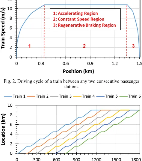
characteristics and load are the same for all of them. The typical speed profile of a certain train between any two virtual stations is shown in Fig. 2, and it is shown that the maximum speed is 38.88km/h. The six trains have the same speed profile that is repeated between any two consecutive passenger stations with the mass of each train remaining the same.
Table I shows the arrival time of the trains at each station, except for station A, where it shows the departure time. It is assumed that the trains are restricted to this timetable and their dwell time in the inter-stations is 30 seconds. The cyclic railway
timetable was first used in 1931 in Netherlands, for passengers’
[image:3.595.313.551.64.190.2]convenience, by making the timetables easy to memorize. Later on, cyclic timetables were adopted by European countries in their bus, metro and railway systems [13]. The positions of the trains against time for the whole journey is shown in Fig. 3. It can be seen that there is an overlap between the trains where a train is braking while another one is accelerating. This overlap plays a very important role in terms of energy exchange and voltage stability. To effectively consume the regenerative braking power for the accelerating trains, the distance between the braking trains and the accelerating trains should be short to minimize losses due to the resistance of the conductor. Consequently, if the traffic density is low and there are not enough trains that can import all of the regenerative braking power, an overvoltage will occur, potentially causing damage to the power network. To protect the system from overvoltage, braking resistors installed on the train are switched in at a defined voltage threshold to dissipate the regenerative power.
Fig. 1. Rail track with 3 substations and 6 running trains.
TABLEI
TIME SCHEDULE OF THE TRAINS IN SECONDS
1 2 3 4 5 6
0 145 290 435 580 725
164 309 454 599 744 889
358 503 648 793 938 1083
552 697 842 987 1132 1277
746 891 1036 1181 1326 1471
940 1085 1230 1375 1520 1665
1134 1279 1424 1569 1714 1859
Station Train Train Train Train Train Train A
[image:3.595.313.550.69.337.2]B C D E F G
Fig. 2. Driving cycle of a train between any two consecutive passenger stations.
Fig. 3. Train diagrams consisting 7 passenger stations.
III. MODEL DESCRIPTION
A. Physical Modelling
In order to move a train from its stationary state, a tractive force needs to be applied. The tractive force decreases when the
train’s speed increases, and depends on many factors such as the
vehicle weight, the gradient, the inclination, and the trip time. Furthermore, the braking force is responsible for bringing the
train to a standstill. While a train is moving, a force – the drag
force – resists its movement, and consists rolling resistance and
air resistance. The equations used in this paper are adopted from [14] as follows:
The drag force Q v( )in
kN
is represented by the Davisequation as
2
( ) .
Q v a bv cv (1)
The coefficients of the Davis equation depend on the train type, when they are calculated experimentally a represents the bearing resistance and is relative to the vehicle mass, b represents the rolling resistance, and c represents the air resistance. The values of the Davis coefficients are available in Table II.
The maximum tractive force
F v
( )
in kN is( ) 310, 10 /
( ) 310 (10 100), 10 22.2 /
F v v m s
F v v v m s
(2)
G
S
u
b
st
a
ti
o
n
3
S
u
b
st
a
ti
o
n
2
S
u
b
st
a
ti
o
n
1
F E D C B A
1.5 km 1.5 km 1.5 km 1.5 km 1.5 km 1.5 km
145 s Headway
[image:3.595.44.283.506.573.2] The maximum electrical braking force
B v
( )
inkN
is( ) 260, 15 /
( ) 260 (18 270), 15 /
B v v m s
B v v v m s
(3)
The train is represented by an ideal current source importing current when it is accelerating or cruising, and exporting current
when it is decelerating. The train’s power demand changes with
time due to the different speed modes, while the auxiliary power is always zero for the sake of simplification. The length of the vehicle is ignored and treated as a particle.
Train dynamics are described in Fig. 4. Grade and curvature resistance are ignored in this model. A PI controller is used to
control the train’s speed to integrate it with the electric power
system. The outputs of the physical model that feed the power system model are the distance travelled by a certain train, and
the train’s current demand (import/export) at that instance. The objective of the electrical model is to be able to simulate the voltage and current along the conductors to analyze the power flow.
B. Electrical Modelling
Substations are based on AC-DC rectification and they are unidirectional. For the reason of considering the DC traction in this study, the AC side of the substation is disregarded and assumed to provide fixed DC voltages. Substations are modelled using ideal DC voltage sources and internal resistances which
represents Thevenin’s equivalent, as shown in Fig. 5. The 3rd and
4th rails are represented by resistive lines. In the figure, the
resistance between the train and the substation is variable, with the distance travelled by the train, and it is represented by the multiplication of the per unit rail electrical resistance and the difference in distance between the train and the substation. The electrical resistance between a certain train and the previous or the next station is a time variant. Furthermore, the other trains running either behind or ahead of a certain train change the electrical resistance value between this train, the next station and the previous station.
The challenge in modelling the electrical system is that the location of the trains is variable, and this causes instantaneous changes to the apparent electrical configuration of the network. Another challenge is that the power demand of the trains also changes with their location. This requires calculation of the voltages and currents at each node along the track. In other words, the network is time-varying, and the circuit equations
change based on the train’s speed and location and the number
[image:4.595.311.549.52.161.2]of trains on the track. The model parameters are shown in Table II.
Fig. 4. Dynamics of a single train.
[image:4.595.42.285.606.681.2]
Fig. 5. Electrical configuration of a train running between two successive substations.
The electrical resistance between a train and the previous station, or the following train, is calculated by (4). Equation (5) can be applied to calculate the electrical resistance between a running train and the next station, or the train ahead if there is one. For example, Fig. 6 shows the electrical resistance difference between train 1 and the next or previous passenger
station. Applying (4) to train 2’s journey results in Fig. 7, and applying (5) to train 2’s journey results in Fig. 8.
'
1 1
'
1 1 1
( ) ( ); ( ) ( ) ( ( ) ( )); ( )
dn d n n n
dn d n n n n
R t R d t d t y
R t R d t d t d t y (4)
''
1 1
''
1 1 1
( ) ( ( )); ( )
( ) ( ( ) ( )); ( )
dn d s n n n
dn d n n n n
R t R d d t d t y
R t R d t d t d t y
(5)
Where, R'dn( )t is the electrical resistance between train
n
and the previous passenger station or the following train, R''dn( )t
is the electrical resistance between train
n
and the nextpassenger station or the train ahead, Rd is the electrical
resistance of the rail track, d tn( ) is the distance travelled by
train
n
which is time variant, and ds is the distance betweenany two consecutive passenger stations, which is always 1.5km in our case. It is worth mentioning that d tn( ) represents the
travelled distance by train
n
between any two consecutivestations, which means that this distance starts at 0km to 1.5km and then repeated until the train finishes its journey. The
travelled distance by a train that is running between train
n
andthe station ahead of train
n
is identified as dn1( )t , and thetravelled distance by a train that is running between train
n
andthe last previous station passed by train
n
is named dn1( )t .Finally, yn1 represents the location of the station ahead of train
n
and yn1 represents the location of the station that was lastlypassed by train
n
.The values of R'dn( )t , and
''
( )
dn
R t are substituted as variable
resistors, that are used to form the electrical model of the railway in Fig. 1. The model and simulation of the 4th rail track was
implemented in MATLAB Simulink. Simscape was used to model the electrical system which was integrated with the physical system. The physical system is responsible for feeding
( )
n
d t and the current demand of the trains to the electrical
model. PI Controller Desired Speed Profile Traction or Braking Force
Acceleration Speed Measured Speed Distance 1 Train Mass Davis Equation Drag Force 1 Constant Train CurrentSubstation1 DC Voltage
Forward Rail Resistance
Substation2 DC Voltage Substation2 Internal Resistance Forward Rail Resistance
Return Rail Resistance Return Rail Resistance
Train Current Substation1
Fig. 6. The electrical resistance between train 1 and the passenger stations.
[image:5.595.44.283.364.496.2]Fig. 7. The electrical resistance difference between train 2 and the train behind or the previous passenger station.
Fig. 8. The electrical resistance difference between train 2 and the train ahead or the next passenger station.
IV. SIMULATION RESULTS AND DISCUSSION
Multiple trains with different scenarios were simulated using the proposed modelling methodology. Interactions between the
trains and power flow based on the track’s voltage have been
shown in Fig. 9. The figure shows the results for six trains. The interactions between the trains are very high due to the short distance between them.
The rapid change of voltage is due to the change in the power demand of a train and also due to the interactions between trains.
During braking mode, the train’s voltage climbs to a value
higher than the substation voltage before it is controlled by the braking resistor box.
The two sections of the railway are electrically isolated by a dead zone called neutral section, which is located at each substation. This sectioning is applied to balance the national grid by drawing power from different phases for adjacent
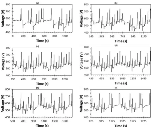
substations. Thus, each rectifier substation is responsible to just feed two adjacent electrical sections. The voltages of the substations are shown in Fig. 10. The voltages of the substations drop below the nominal voltage when the trains accelerate close to them, and the voltages rise when the trains decelerate close to the substations.
It is noticed that between the three substations, substation 2, which is located in the middle of the track, is producing more power than the others. The mean power of the substations is 0.5MW, 0.73MW, and 0.29MW respectively. The traction substation 2 supplies more power because, in most cases, it is closer to the accelerating trains than the other two traction substations. Similarly, the highest peak power occurs at substation 2 with a value of 3.15MW.
[image:5.595.336.551.484.728.2]Fig. 10. The substations’ voltages: (a) substation 1; (b) substation 2; (c) substation 3.
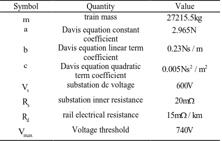
TABLEII
PARAMETERS OF THE TRAINS AND THE ELECTRIC RAILWAY SYSTEM
Symbol Quantity Value
m train mass 27215.5kg
a Davis equation constant coefficient
2.965N
b Davis equation linear term coefficient
0.23Ns m /
c Davis equation quadratic term coefficient
2 2
0.005Ns /m
s
V substation dc voltage 600V
s
R substation inner resistance 20m
d
R rail electrical resistance 15m/km
max
V Voltage threshold 740V
Fig. 11 shows the total wasted energy in the braking resistors for the same system but with different departure intervals. It can be seen that increasing the headway increases the losses in the braking resistors because the trains running at a low traffic density. Headway is crucial to optimize energy efficiency in multi-train railways. Furthermore, storing the regenerative energy in ESSs instead of dissipating it in the braking resistors can be used to improve the energy efficiency of the railway. The unused braking energy of each train is calculated by
0
T cb cb train
E I V dt
(6)
where Icb is the current passing through the braking resistor of
the train, and Vtrain is the voltage seen by the train.
Effective power exchange between the running trains can reduce the power consumption of the rectifier substations, therefore the utilization of the regenerative energy should be considered for the study into ESSs. The utilization factor
utilization measures the percentage of the used braking energy outof the total braking energy, as follows
100%
r cbutilization
r
E E
E
(7)
where
Er is the total regenerative energy by the brakingtrains and
Ecb is the total dissipated braking energy in thebraking resistors of the trains.
The utilization factor for the case study above is 77%, meaning that minimal energy was wasted in the braking
resistors, due to the high traffic density. Fig. 12 shows the receptivity of the railway line, which is the capability of the trains to accept the available regenerative energy by decelerating trains. It is observed that the line’s receptivity reduces with increasing headway. In decoupled railways, the receptivity of the lines deteriorates with the increase of headway due to the high likelihood of consecutive trains being separated by different electrical sections, which is the case for 550s headway. However, if all of the trains start accelerating and decelerating together, then the wasted energy in the onboard braking resistors will be very high and the utilization factor will be very low despite the fact that the headway is small. It is concluded that the lower number of trains running simultaneously on the track results in lower power utilization in the railway. Similarly, increasing the headway of multi-trains decreases the power utilization in the railway.
V. VALIDATION
The passenger stations are situated at different locations along the track, and they are stationary. The trains are moving with time and they all pass these stations at a known time.
Measuring the passenger stations’ voltages and the voltages
[image:6.595.65.284.53.172.2]experienced by the trains, these should be matched at that time when a train is located at a certain station. From Table I, it is known that train 1 reaches interstation F at 940s and dwells for 30s, and during this time, voltage matching occurs as shown in Fig. 13. Another case is considered in Fig. 14, which shows a
match between the virtual station’s voltage and the train’s
voltage when the train and the station have the same location on the track. Noticeably, high voltage calculation accuracy is proved notwithstanding the dynamic behavior of the electric railway.
Another method to validate the model is summing the total energy, which should be equal to zero. In other words, the
substations’ output energy and the trains’ regenerative energy should equal to the trains’ energy consumption, and the total
losses in the system as follows
_ _
Es
Er
Et
Eline losses
Esubstation losses
Ecb (8)where
Es is the total energy consumption of all of thesubstations;
Er is the total regenerative energy by thebraking trains;
Et is the total traction energy consumed by allof the trains;
Eline losses_ is the total energy losses in the 3rdand 4th rail; and
Esubstation losses_ is the total energy losses in the internal resistors of the substations;._ _
( ) ( ) ( ) ( ) ( ) ( )
857.94 207.5 893.06 82.44 50.76 47.69
E kWhs E kWhr E kWht Eline losseskWh Esubstation losseskWh EcbkWh
[image:6.595.53.274.230.371.2]Fig. 11. The total energy dissipated through the onboard braking resistors with respect to changing the headway.
Fig. 12. The receptivity of the railway line to accept the available regenerative energy with respect to changing the headway.
Fig. 13. Measured voltage at station F and voltage seen by train 1.
Fig. 14. Measured voltage at station B and voltage seen by train 3.
VI. CONCLUSION
The purpose of this paper was to develop an electrical model that describes the effect of a moving train over an electric DC railway. The work has presented a simplified test scenario of 6 trains running on a 9km rail track in order to show validation of the model against the expected observations. The model can provide the track and train voltages at any location along with power flows. This model can therefore be used to study the effects of energy storage on the railway system and to optimize it for solutions. Consequently, it will be possible to design onboard or stationary ESSs to import and export energy with accurate energy calculations by voltage control. The proposed simulation method is simple, accurate, and adaptable to changes in the circuit configuration. As a consequence of this method, iterative math methods to solve the nonlinear equations of the system have been avoided.
REFERENCES
[1] H. Al-Ezee, S. B. Tennakoon, I. Taylor, and D. Scheidecker, “Aspects of catenary free operation of DC traction systems,” Proc. Univ. Power Eng. Conf., vol. 2015–Novem, 2015.
[2] C. J. Goodman, “Overview of Electric Railway Systems and the Calculation of Train Performance,” 9th IET Prof. Dev. Course Electr. Tract. Syst., pp. 13–36, 2006.
[3] A. Zaboli, B. Vahidi, S. Yousefi, and M. M. Hosseini-Biyouki, “Evaluation and Control of Stray Current in DC-Electrified Railway Systems,” IEEE Trans. Veh. Technol., vol. 66, no. 2, pp. 974–980, 2017.
[4] C. S. Chen, H. J. Chuang, and J. L. Chen, “Analysis of dynamic load behavior for electrified mass rapid\ntransit systems,” Conf. Rec. 1999 IEEE Ind. Appl. Conf. Thirty-Forth IAS Annu. Meet. (Cat. No.99CH36370), vol. 2, pp. 992–998, 1999.
[5] H. Xia, H. Chen, Z. Yang, F. Lin, and B. Wang, “Optimal energy management, location and size for stationary energy storage system in a metro line based on genetic algorithm,” Energies, vol. 8, no. 10, pp. 11618–11640, 2015.
[6] T. Kulworawanichpong, “Multi-train modeling and simulation integrated with traction power supply solver using simplified Newton-Raphson method,” J. Med. Biol. Eng., vol. 35, no. 6, pp. 241–251, 2015.
[7] B. Mohamed, P. Arboleya, and C. Gonzalez-Moran, “Modified Current Injection Method for Power Flow Analysis in Heavy-Meshed DC Railway Networks with Nonreversible Substations,” IEEE Trans. Veh. Technol., vol. 66, no. 9, pp. 7688–7696, 2017. [8] B. R. Ke, K. L. Lian, Y. L. Ke, T. H. Huang, and M. R.
Mirwandhana, “Control strategies for improving energy efficiency of train operation and reducing DC traction peak power in mass Rapid Transit System,” 2017 IEEE/IAS 53rd Ind. Commer. Power Syst. Tech. Conf. I CPS 2017, pp. 1–9, 2017.
[9] Z. Tian et al., “Energy evaluation of the power network of a DC railway system with regenerating trains,” IET Electr. Syst. Transp., vol. 6, no. 2, pp. 41–49, 2016.
[image:7.595.46.534.289.698.2] [image:7.595.48.354.397.689.2][10] S. Watanabe and T. Koseki, “Train group control for energy-saving DC-electric railway operation,” 2014 Int. Power Electron. Conf. IPEC-Hiroshima - ECCE Asia 2014, pp. 1334–1341, 2014. [11] P. Arboleya, M. Coto, C. González-Morán, and R. Arregui, “On
board accumulator model for power flow studies in DC traction networks,” Electr. Power Syst. Res., vol. 116, pp. 266–275, 2014. [12] R. Barrero, X. Tackoen, and J. Van Mierlo, “Quasi-static simulation
method for evaluation of energy consumption in hybrid light rail vehicles,” IEEE Veh. Power Propuls. Conf., 2008.
[13] L. W. Peeters, “Cyclic railway timetable optimization,” Ph. D., Erasmus Universiteit Rotterdam, June 2003.