Antarctic pack ice algal distribution: Floe-scale
spatial variability and predictability
from physical parameters
K. M. Meiners1,2 , S. Arndt3 , S. Bestley4 , T. Krumpen3 , R. Ricker3,5 , M. Milnes1, K. Newbery1, U. Freier6, S. Jarman1,7 , R. King1, R. Proud8 , S. Kawaguchi1,2, and B. Meyer9,10,11
1
Department of the Environment and Energy, Australian Antarctic Division, Kingston, Tasmania, Australia,2Antarctic Climate and Ecosystems Cooperative Research Centre, University of Tasmania, Hobart, Tasmania, Australia,3Sea Ice Physics, Alfred Wegener Institute, Helmholtz Centre for Polar and Marine Research, Bremerhaven, Germany,4Institute for Marine and Antarctic Studies, University of Tasmania, Hobart, Tasmania, Australia,5Laboratoire d’Océanographie Physique et Spatiale, IUEM, University of Brest, CNRS, IRD, Ifremer, Brest, France,6SC-Scientific Consulting, Neuss, Germany,7 CIBIO-InBIO, Centro de Investigação em Biodiversidade e Recursos Genéticos, Universidade do Porto, Vairão, Portugal,8Pelagic Ecology Research Group, Scottish Oceans Institute, Gatty Marine Laboratory, University of St Andrews, Scotland, UK,9Polar Biological Oceanography, Alfred Wegener Institute, Helmholtz Centre for Polar and Marine Research, Bremerhaven, Germany,10Institute for Chemistry and Biology of the Marine Environment, Carl von Ossietzky University of Oldenburg, Oldenburg, Germany,11Helmholtz Institute for Functional Marine Biodiversity, Oldenburg, Germany
Abstract
Antarctic pack ice serves as habitat for microalgae which contribute to Southern Ocean primary production and serve as important food source for pelagic herbivores. Ice algal biomass is highly patchy and remains severely undersampled by classical methods such as spatially restricted ice coring surveys. Here we provide an unprecedented view of ice algal biomass distribution, mapped (as chlorophylla) in a 100 m by 100 m area of a Weddell Sea pack icefloe, using under-ice irradiance measurements taken with an instrumented remotely operated vehicle. We identified significant correlations (p<0.001) between algal biomass and concomitant in situ surface measurements of snow depth, ice thickness, and estimated sea ice freeboard levels using a statistical model. The model’s explanatory power (r2= 0.30) indicates that these parameters alone may provide afirst basis for spatial prediction of ice algal biomass, but parameterization of additional determinants is needed to inform more robust upscaling efforts.1. Introduction
Sea ice is a key driver of Southern Ocean physical and biogeochemical processes and plays a pivotal role in Antarctic marine ecosystem function [Thomas, 2017]. Antarctic pack ice provides a vast habitat for ice-associated algae which form distinct communities in surface, interior, and bottom layers of sea icefloes [Meiners et al., 2012;Arrigo, 2017]. Model estimates suggest that sea ice algal production can contribute significantly to the overall annual primary production of the ice-covered Southern Ocean [Saenz and Arrigo, 2014]. However, modeled ice algal production and biomass estimates are subject to considerable uncertainty asfield-based observations of ice algal biomass, necessary to evaluate ecosystem models, remain extremely sparse [Meiners et al., 2012]. The high spatial heterogeneity of ice algal distribution averts reliable in situ biomass estimation with classical methods, such as ice core sampling, on relevant scales, e.g., for local-regional estimates of biomass [Mundy et al., 2007;Lange et al., 2016].
Physical sea ice properties, such as snow depth, ice thickness, and surface slush layers, are considered key factors in controlling ice algal biomass [Eicken, 1992;Fritsen et al., 1998;Mundy et al., 2005;Vancoppenolle et al., 2013], but their role in driving the floe-scale spatial distribution of pack ice algae remains poorly understood. Snow on Antarctic pack ice, for example, reduces light needed for algal photosynthesis but can also suppress pack icefloes below seawater levels, thereby replenishing nutrients and promoting algal growth in surface slush and refrozen slush (= snow ice) layers [Fritsen et al., 1998; Arrigo et al., 2014]. Scavenging of phytoplankton by frazil crystals during ice formation can result in the development of interior communities [Spindler, 1994], which can also emerge during ridging and rafting [Ackley and Sullivan, 1994]. While generally lower in biomass than bottom and surface communities, interior communities can significantly contribute to integrated biomass values [Meiners et al., 2012]. Thus, thicker sea ice may be associated with increased integrated ice algal biomass [Meiners et al., 2011;Arrigo et al., 2014]. Improving
Geophysical Research Letters
RESEARCH LETTER
10.1002/2017GL074346Key Points:
•First map of thefloe-scale distribution of ice algal chlorophyllain Antarctic pack ice established
•Snow depth, ice thickness, and sea ice freeboard levels significantly affect ice algal chlorophylladistribution
•Described relationships provide afirst step toward upscaling, i.e.,
predictability of ice algal biomass from sea ice physical parameters
Supporting Information:
•Supporting Information S1
Correspondence to: K. M. Meiners,
Citation:
Meiners, K. M., et al. (2017), Antarctic pack ice algal distribution: Floe-scale spatial variability and predictability from physical parameters,Geophys. Res. Lett., 44, 7382–7390, doi:10.1002/
2017GL074346.
Received 29 MAY 2017 Accepted 11 JUL 2017
Accepted article online 14 JUL 2017 Published online 29 JUL 2017
measurement capabilities to simultaneously determine sea ice physical properties and in situ ice algal biomass, and establishing statistical relationships between these parameters, is necessary to develop and test the feasibility of upscaling efforts. The ultimate goal of such efforts would be estimation of ice algal biomass from remotely sensed estimates of physical sea ice properties, such as emerging satellite products for snow depth and ice thickness.
The presence of ice algal photosynthetic pigments affects under-ice irradiance spectra through absorption of specific wavelengths in the photosynthetic active radiation (400–700 nm) range [e.g.,Perovich et al., 1993; Arrigo and Sullivan, 1994;Fritsen et al., 2011;Hawes et al., 2012;Lange et al., 2016]. Changes in spectra, often characterized by the difference of intensities at two key wavelengths, have been used to develop algorithms to estimate sea ice algal chlorophylla(chla, as proxy for biomass) from under-ice spectra collected with moored and horizontally profiling instruments [Mundy et al., 2007;Campbell et al., 2015;Lange et al., 2016]. Employing a normalized difference index (NDI) approach,Melbourne-Thomas et al. [2015, 2016] recently established an NDI algorithm to estimate ice algal chlain Weddell Sea pack ice from irradiance spectra measured beneath sea ice. This algorithm accounted for 79% of the total variation of integrated ice algal chlain Weddell Sea pack ice.
Recent advance in the development of underwater vehicles and under-ice trawls has provided new opportunities to study sea ice physical and biological properties on small to medium scales (up to 1000 m). These include measurements and mapping of sea ice draft [Wadhams and Doble, 2008;Williams et al., 2013, 2015] and light transmission [Nicolaus et al., 2012;Nicolaus and Katlein, 2013;Katlein et al., 2015a;Arndt et al., 2017]. Biological properties such as the distribution of bottom-ice algae and under-ice algal aggregates [Gutt, 1995;Katlein et al., 2015b], and most recently integrated ice algal biomass [Lange et al., 2016], have also been determined.
In this study, we present thefirst map of the chlaconcentration of an Antarctic pack icefloe in a 100 m by 100 m area. We analyzed these data in combination with concomitant surface measurements of snow depth, sea ice thickness, and calculated sea ice freeboard estimates in afirst attempt to identify physical controls of the distribution of Antarctic pack ice algal biomass at the sea icefloe scale.
2. Material and Methods
2.1. Study Site and Field ProceduresSampling was carried out as part of the“Winter Ice Study on Key Species”experiment in the Weddell Sea dur-ing late austral winter-early austral sprdur-ing 2013 on the German icebreaker R/VPolarstern(voyage ANTXXIX-7/ PS81). The study site was at an approximate position of 60.78°S and 26.36°W and located in the center of a deformed first year pack icefloe composed of smaller icefloes frozen together [Meyer and Auerswald, 2014]. Remotely operated vehicle (ROV) and concomitant surface surveys were conducted as outlined in detail in a related paper on light transmission through Antarctic pack ice [Arndt et al., 2017] (see also support-ing information). Briefly, under-ice irradiance spectra were collected with a ROV equipped with an upward looking hyperspectral radiometer (TriOS, Ramses-ACC) in a designated 100 m by 100 m area during 17 deployments between 18 and 26 September 2013. Atmospheric and ice surface conditions remained stable during this period [Arndt et al., 2017], which allowed merging of all observations for the following analyses. A Long Base Line positioning system, interrogating four ice-tethered transponders, coupled to GPS units (at the ice surface), and spaced around the survey site in a 400 m by 400 m rectangle, was used to determine and capture the ROV position data [e.g.,Williams et al., 2015] (for details, see supporting information). The surface GPS data allowed for precise registration of any icefloe drift and rotation in between ROV and surface surveys and were used to merge under-ice survey data with the temporally displaced surface measurements. Snow depth and total ice thickness measurements were conducted on a single day after completion of the last ROV survey to prevent disturbance of the snow surface features. A sled-mounted, GPS-enabled, multifrequency electromagnetic induction instrument (GEM-2, Geophex Ltd.) [Hunkeler et al., 2015] was used to measure total ice thickness (sea ice thickness plus snow depth) in the ROV grid. Snow depths were measured every two steps along the GEM-2 tracks using a GPS-equipped Snow Depth Probe (Snow-Hydro, USA).
algorithm [Melbourne-Thomas et al., 2015, 2016]. For full details of the sample site selection and NDI evaluation, see the supporting information. Field-based under-ice irradiance measurements, ice core collection, andfluorometric in vitro analysis of ice algal chlaexactly followed the methods outlined in Melbourne-Thomas et al. [2015].
2.2. Data Preparation
Analysis of under-ice irradiances was restricted to ROV radiometer data with a distance of≤2 m to the sea ice subsurface, resulting in 4482 valid under-ice spectra along 17 dive tracks. All ROV measurements taken within an area of 2 m by 2 m were averaged to account for ROV track overlap [Arndt et al., 2017]. All grid cells overlap for 1 m translating to an effective grid resolution of 1 m (running mean).
Ice thickness was calculated from the total snow + ice GEM-2 data by subtraction of the Snow Depth Probe data from the GEM-2 data. Using nearest neighbor resampling, we interpolated these surface measurements to the positions of the under-ice irradiance measurements.
Sea ice freeboard levels are controlled by the buoyancy of sea ice and the mass of the snow load. We calculated freeboard levels as a function of snow depth and ice thickness using mean density values for seawater, sea ice, and snow [Yi et al., 2011; Arndt et al., 2017] (for details, see supporting information). Negative freeboard values indicate flooding, while negative freeboard magnitudes specify the slush layer thickness.
Collected broadband hyperspectral under-ice irradiance spectra were interpolated to a spectral resolution of 1 nm. From these we calculated the optically derived integrated ice algal biomass values (ChlaROV, mg m 2), using the established NDI to ice algal chlarelationship ofMelbourne-Thomas et al. [2015, 2016], as detailed in the supporting information (Figure S1).
2.3. Statistical Analyses
Empirical variograms were used to explore scales of spatial variability in physical and biological data sets. Variograms describe the variance in spatially binned subsets of the data as a function of varying distances (lag distances). Theoretical exponential variograms werefitted to estimate variogram“range”parameters, i.e., the lag distance at which the modelflattens out and reaches 95% of its sill value [Cressie, 1991]. The range value provides a measure of the spatial autocorrelation length scale of the respective parameter.
To analyze the relationship between ice algal biomass and sea ice physical parameters (snow depth, ice thick-ness, and sea ice freeboard as predictor variables), we employed a Generalized Additive Model approach (GAM) [Wood, 2006], as relationships were not necessarily expected to be linear, using themgcvR package [Wood, 2016]. A Gaussian error distribution was used, with the Chl aROV and ice thickness values log transformed prior to analysis to normalize the residuals. Outliers at very high and low values of ice thickness and snow depth were removed (1.27% of total data). Spatially autocorrelated data can affect the smoothness estimation of model terms; i.e., the estimation procedure in GAM is likely to undersmooth. We therefore also implemented the same model including a spatial term interaction onxandy(full tensor product smooth). This model (GAMxy) accounted for effects of ROV position,xandyvalues, minimizing the effects of spatial autocorrelation on the estimation for the physical parameters (supporting information Figure S2). Significance levels were evaluated usingFstatistics [Wood, 2006]. GAM analyses were conducted using the statistical software R (version 3.3.1, R Development Core Team, 2016).
3. Results and Discussion
3.1. Point Measurements3.2. Spatial Survey
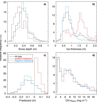
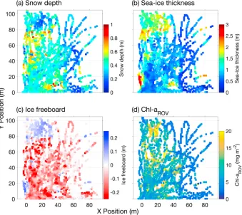
The area surveyed by ROV was part of a large (>1 km2)first year pack icefloe showing highly variable snow depths and ice thicknesses (Figures 1 and 2) and situated in a band of dense pack ice. The study site demonstrated substantial snow accumulation with snow depth ranging from 0.08 m to 0.91 m (mean = 0.39 ± 0.13 m) and a modal snow depth of 0.39 m (Figures 1a and 2a). Sea ice thickness varied between 0.03 m and 2.57 m (mean = 0.93 ± 0.45 m, mode = 0.79 m) with a noteworthy contribution of thicker sea ice as indicated by the tail in the frequency distribution (Figure 1b). Thick sea ice was observed in distinct clusters denoting localized deformation features (Figure 2b). Measured snow depths and ice thicknesses were higher but broadly consistent with climatological mean snow depth and ice thickness values for eastern Weddell Sea pack ice as reported in the ASPeCt observations data set [Worby et al., 2008], the most comprehensive data compilation available. The sampled sea ice area was thus characteristic for a deformed first year Antarctic pack icefloe with heavy snow cover. The heavy snow load resulted in widespreadflooding and occurrence of slush layers, as observed during sampling and indicated by the large proportion (76.8%) of negative values in calculated freeboard levels (Figures 1c and 2c). Widespreadflooding is a key feature of Weddell Sea ice [Lange et al., 1990] and more generally Antarctic pack ice [Sturm and Massom, 2017]. Snow depth distributions were similar overall for negative and positive freeboard levels, albeit snow depths
[image:4.612.206.545.87.442.2]variable and ranged over 0.4 m to 2.5 m. Within the survey area, the 2-D distribution of sea ice freeboard levels showed general agreement with the distribution of sea ice thickness (Figures 2b and 2c), although estimated autocorrelation length scales, i.e., variogram ranges, were distinctly different with values of 28.8 m, 41.7 m, and 19.6 m for snow depth, ice thickness, and freeboard levels, respectively (Figure 3).
Estimated integrated ice algal chlaconcentrations (ChlaROV, calculated according toMelbourne-Thomas
et al. [2015, 2016]) ranged from 1.96 to 19.95 mg m 2(mean = 7.22 ± 4.00 mg m 2) with a median value of 6.62 mg m 2. This relatively large range contrasts the smaller range encountered in the data set forfive ice cores sampled from this icefloe (supporting information Figure S1). Classical ice coring surveys typi-cally collect only a small number of cores [Miller et al., 2015]. Our results highlight that small ice core sam-ple sizes might result in large biases offloe-scale ice algal biomass estimates due to insufficient spatial representation of the collected ice cores. This has recently been discussed in detail by Lange et al. [2016] for Arctic pack ice. The ChlaROVvalues showed a highly skewed frequency distribution with a high relative contribution of low values (Figure 1d), consistent with the ASPeCt-Bio observational data set in which about 50% of all ice cores (n = 1300) show an integrated ice algal chl a value of <3 mg m 2 [Meiners et al., 2012].
[image:5.612.206.545.91.393.2]The map of ChlaROVshows a highly variable distribution with no simple association to the spatial distribution of snow depth, ice thickness, or freeboard levels (Figure 2d). The variogram-based range value for ChlaROVis 17.3 m (Figure 3), which may provide some indication of the“patch”scale of integrated ice algal biomass in the studied sea icefloe. The difference between this range and the calculated range values for snow depth, ice thickness, and freeboard levels highlights the complexity in relationships between sea ice physical parameters and ice algal biomass as reported in previous studies and reviews [e.g.,Arrigo, 2014;Meiners Figure 2.Spatial distribution of sea ice physical properties and ice algal biomass in the ROV survey area. (a) Snow depth as measured with the Snow Depth Probe, (b) ice thickness calculated from the GEM-2 measurements, (c) ice freeboard levels calculated as function of snow depth and ice thickness (for details see text), and (d) integrated ice algal biomass as chlorophylla(ChlaROV) determined from under-ice irradiance measurements using the algorithm by
and Michel, 2017;Thomas, 2017]. Snow on sea ice, for example, influences ice algal biomass in multiple ways. Due to its high albedo and light attenuation properties, snow is a key factor controlling the light available to ice algal communities [Leu et al., 2015;Campbell et al., 2015]. Early in the growth season, snow cover can result in light limitation of ice algal growth, whereas later in the season snow cover can prevent photoinhibition of ice algal communities which are generally shade adapted [Arrigo, 2014, 2017]. In addition, snow cover can insulate sea ice, thus preventing internal ice melting and bottom ablation [Sturm and Massom, 2017], thereby stabilizing ice algal habitats. In the present study, integrated ice algal biomass (ChlaROV) was negatively correlated with snow depth, particularly at snow depths above 0.4 m (GAM:s(Zsnow),p<0.0001, Figure 4a; GAMxy:s(Zsnow),p= 0.007; supporting information Figure S2a), which is consistent with the light-limiting role of snow during the winter-early spring transition. Our late-winter/early-spring data (September) contrast with summer (December–January) results of Arrigo et al. [2014], which showed a positive relationship between snow depth and integrated ice algal biomass for Amundsen Sea ice. In combination, these studies support the notion of a seasonally changing influence of snow on ice algal biomass in the Antarctic pack ice zone, as recently shown for Arctic landfast sea ice [Leu et al., 2015;Campbell et al., 2015]. We hypothesize that early in the season snow on Antarctic pack ice limits ice algal accumulation, while later in the season snow cover supports ice algal accumulation.
ChlaROVshowed a positive correlation with sea ice thickness (GAM:s(log[Zice]),p<0.0001, Figure 4b; GAMxy: s(log[Zice]),p<0.0001; supporting information Figure S2b), particularly at an ice thickness above 1 m. Internal ice algal communities are a key feature of Antarctic pack ice [Arrigo, 2017] and have previously been shown to have an increased probability of occurrence in thicker sea ice, e.g., due to sea ice deformation processes such as rafting [Ackley and Sullivan, 1994;Meiners et al., 2012]. Moreover, microalgae are incorporated into sea ice during ice formation through various processes including scavenging [Spindler, 1994] and retention of particulate material during thermodynamic ice growth [Janssens et al., 2016]. Thus, most Antarctic pack ice types contain at least low levels of algal chla, and an increase in sea ice thickness results in an increase in integrated chlavalues.
[image:6.612.218.529.88.331.2]We note that our GAM analyses suggest a likely interaction between ice thickness and snow depth, whereby thicker ice can support higher snow loadings. This may moderate the negative snow effects on integrated algal biomass early in the season and allows for thefinal outcome that thicker ice harbors more integrated Figure 3.Variograms for (a) snow depth, (b) ice thickness, (c) calculated freeboard level, and (d) integrated ice algal biomass (as chlorophylladetermined from under-ice irradiance measurement (ChlaROV)). Open circles with black lines
algal biomass even with a higher snow load. Our data set contains a low amount of data (<2.4%) with high (>2.0 m) and low (<0.2 m) ice thicknesses. Future surveys of a larger range of ice thicknesses would be valuable to explore this observation and determine potential thresholds.
Surface flooding and subsequent snow ice formation are estimated to affect large parts of the Antarctic ice pack [Wadhams et al., 1987; Sturm and Massom, 2017], and snow ice is considered to contribute a significant proportion to the total Antarctic sea ice volume [Jeffries et al., 1998; Maksym and Markus, 2008]. The flooding water may originate from sea ice brines, if the ice is permeable [Golden et al., 1998; Jutras et al., 2016], or can be seawater moving laterally from ice floe edges and cracks [Massom et al., 2001]. Flooding of snow and surface ice may seed these layers with microalgae and increases nutrient availability. Both field observations [Fritsen et al., 1994] and modeling studies [Saenz and Arrigo, 2012, 2014] suggest that surface flooding and freeze cycles are critically important for ice algal biomass accumulation in Antarctic pack ice surface layers. Consistent with these studies, the Chl aROV data in our study were significantly negatively correlated with calculated freeboard levels (GAM: s(FB), p < 0.0001, Figure 4c; GAMxy:
s(FB), p < 0.0001; supporting information Figure S2c), i.e., potentiallyflooded areas with slush layers showed increased integrated ice algal biomass.
3.3. Conclusion
In conclusion, our study provides an unprecedented view of the spatial variability of ice algal biomass (as chl a) in Antarctic pack ice and constitutes an important step toward estimating ice algal biomass from sea ice physical parameters. We observed a large difference between the mean and range of ice algal biomass estimates based on ice core sampling versus optically derived measurements, further highlighting the Figure 4.Smooths of generalized additive modeling (GAM) terms showing
the effect of physical parameters on integrated ice algal biomass (ChlaROV,
uncertainty in ice algal biomass estimates from limited ice coring surveys [Lange et al., 2016]. We suggest that newly available methods forfloe-scale ice algal biomass estimation, e.g., using instrumented underwater vehicles as demonstrated in this study, will be better suited for comprehensive biomass estimates on relevant spatial scales.
Our GAM analyses showed highly significant floe-scale relationships between measured physical sea ice properties and integrated ice algal biomass for this late-winter/early-spring Antarctic pack ice study. The model had moderate explanatory power (GAM: R2adj = 0.30, 30.8% of the deviance explained; GAMxy:
R2adj= 0.55, 55.7% of the deviance explained), considering the relatively few predictor variables. This suggests feasibility of spatial upscaling, such as the estimation of local-to-regional Antarctic ice algal biomass from emerging remote sensing snow depth and ice thickness products [Kurtz and Markus, 2012]. Such advances promise a new independent way to estimate ice algal biomass and will help to inform and evaluate ice algal primary production models. However, broad-scale prediction of Antarctic pack ice algal biomass from physical sea ice properties alone needs further assessment. To achieve this, an improved knowledge of the spatial variability of ice algal biomass and an improved understanding of the temporal scales of coupling/decoupling between sea ice physical processes and ice algal biomass development are both required. Furthermore, additional physical sea ice properties, such as under-ice rugosity and sea ice temperature (as proxy for porosity), which are expected to influence ice algal distribution need to be measured and accounted for. The ready availability and swift emergence of underwater vehicle technologies should support a rapid proliferation of independent data sets at local-to-regional scales, and enable sampling of a wider range of icescapes as well as targeting seasonal differences and progressions.
References
Ackley, S. F., and C. W. Sullivan (1994), Physical controls on the development and characteristics of Antarctic sea ice biological communities
—A review and synthesis,Deep Sea Res., Part I,41, 1583–1604.
Arndt, S., K. M. Meiners, R. Ricker, T. Krumpen, C. Katlein, and M. Nicolaus (2017), Influence of snow depth and surfaceflooding on light transmission through Antarctic pack ice,J. Geophys. Res. Oceans,122, 2108–2119, doi:10.1002/2016JC012325.
Arrigo, K. R. (2014), Sea ice ecosystems,Annu. Rev. Mar. Sci.,6, 439–467.
Arrigo, K. R. (2017), Sea ice as a habitat for primary producers, inSea Ice, 3rd ed., edited by D. N. Thomas, pp. 352–369, Wiley and Blackwell Ltd., Oxford, U. K.
Arrigo, K. R., and C. W. Sullivan (1994), A high resolution bio-optical model of microalgal growth: Tests using sea-ice algal community time-series data,Limnol. Oceanogr.,39, 609–663.
Arrigo, K. R., Z. B. Brown, and M. M. Mills (2014), Sea ice algal biomass and physiology in the Amundsen Sea, Antarctica,Elem. Sci. Anth.,2, 000028, doi:10.12952/journal.elementa.000028.
Campbell, K., C. J. Mundy, D. G. Barber, and M. Gosselin (2015), Characterizing the sea ice algae chlorophylla—snow depth relationship over Arctic spring melt using transmitted irradiance,J. Mar. Syst.,147, 76–84.
Cressie, N. (1991),Statistics for Spatial Data, 900 pp., John Wiley, New York.
Eicken, H. (1992), The role of sea ice in structuring Antarctic ecosystems,Polar Biol.,12, 3–13, doi:10.1007/BF00239960.
Fritsen, C. H., V. I. Lytle, S. F. Ackley, and C. W. Sullivan (1994), Autumn bloom of Antarctic pack-ice algae,Science,266(5186), 782–784, doi:10.1126/science.266.5186.782.
Fritsen, C. H., S. F. Ackley, J. N. Kremer, and C. W. Sullivan (1998), Flood-freeze cycles and microalgal dynamics in Antarctic pack ice, in Antarctic Sea Ice: Biological Processes, Interactions and Variability,Antarct. Res. Ser., vol. 73, edited by M. P. Lizotte and K. R. Arrigo, pp. 1–22, AGU, Washington, D. C.
Fritsen, C. H., E. D. Wirthlin, D. K. Momberg, M. J. Lewis, and S. F. Ackley (2011), Bio-optical properties of Antarctic pack ice in the early austral spring,Deep Sea Res., Part II,58, 1052–1061.
Golden, K. M., S. F. Ackley, and V. I. Lytle (1998), The percolation phase transition in sea ice,Science,282, 2238–2241. Gutt, J. (1995), The occurrence of sub-ice algal aggregations off northeast Greenland,Polar Biol.,15, 247–252.
Hawes, I., L. C. Lund-Hansen, B. K. Sorrell, M. Holtegaard Nielsen, R. Borzák, and I. Buss (2012), Photobiology of sea ice algae during initial spring growth in Kangerlussuaq, West Greenland: Insights from imaging variable chlorophyllfluorescence of ice cores,Photosynth. Res., 112, 103–115.
Hunkeler, P. A., S. Hendricks, M. Hoppmann, S. Paul, and R. Gerdes (2015), Towards an estimation of sub-sea-ice platelet-layer volume with multi-frequency electromagnetic induction sounding,Ann. Glaciol.,56, 137–146.
Janssens, J., K. M. Meiners, J. L. Tison, G. S. Dieckmann, B. Delille, and D. Lannuzel (2016), Incorporation of iron and organic matter into young Antarctic sea ice during its initial growth stages,Elem. Sci. Anth.,4, doi:10.12952/journal.elementa.000123.
Jeffries, M. O., S. Li, R. A. Jana, H. R. Krouse, and B. Hurst-Cushing (1998), Late winterfirst-year icefloe thickness variability, seawaterflooding and snow ice formation in the Amundsen and Ross Seas, inAntarctic Sea Ice: Physical Processes, Interactions and Variability,Antarct. Res. Ser., vol. 74, edited by O. Jeffries, pp. 69–87, AGU, Washington D. C.
Jutras, M., M. Vancoppenolle, A. Lourenço, F. Vivier, G. Carnat, G. Madec, C. Rousset, and J.-L. Tison (2016), Thermodynamics of slush and snow–ice formation in the Antarctic sea-ice zone,Deep Sea Res., Part II,131, 75–83.
Katlein, C., M. Fernández-Méndez, F. Wenzhöfer, and M. Nicolaus (2015a), Distribution of algal aggregates under summer sea ice in the Central Arctic,Polar Biol.,38, 719–731.
Katlein, C., et al. (2015b), Influence of ice thickness and surface properties on light transmission through Arctic sea ice,J. Geophys. Res. Oceans,120, 5932–5944, doi:10.1002/2015JC010914.
Acknowledgments
We thank the captain, crew, and shipboard scientific party ofPolarstern voyage ANTXXIX-7/PS89 for their support of our work. We gratefully acknowledge the Australian Antarctic Division’s Science Technical Support and Instrument Workshop teams and in particular Peter Mantel, for their expert help in instrumenting, ice hardening, and piloting the ROV. This study was supported by the PACES (Polar Regions and Coasts in a changing Earth System) program (Topic 1, WP 5) of the Alfred Wegener Institute, Helmholtz Centre for Polar and Marine Research, the Helmholtz Virtual Institute“PolarTime” (VH-VI-500: Biological timing in a changing marine environment—Clocks and rhythms in polar pelagic organisms), the Helmholtz Alliance
Kurtz, N. T., and T. Markus (2012), Satellite observations of Antarctic sea ice thickness and volume,J. Geophys. Res.,117, C08025, doi:10.1029/ 2012JC008141.
Lange, B. A., C. Katlein, M. Nicolaus, I. Peeken, and H. Flores (2016), Sea ice algae chlorophyllaconcentrations derived from under-ice spectral radiation profiling platforms,J. Geophys. Res. Oceans,121, 8511–8534, doi:10.1002/2016JC011991.
Lange, M. A., P. Schlosser, S. F. Ackley, P. Wadhams, and G. S. Dieckmann (1990),18O concentrations in sea ice of the Weddell Sea, Antarctica, J. Glaciol.,36, 315–323.
Leu, E., C. J. Mundy, P. Assmy, K. Campbell, T. M. Gabrielsen, M. Gosselin, T. Juul-Pedersen, and R. Gradinger (2015), Arctic spring awakening— Steering principles behind the phenology of vernal ice algal blooms,Prog. Oceanogr.,139, 151–170.
Maksym, T., and T. Markus (2008), Antarctic sea ice thickness and snow-to-ice conversion from atmospheric reanalysis and passive microwave snow depth,J. Geophys. Res.,113, C02S12, doi:10.1029/2006JC004085.
Massom, R. A., et al. (2001), Snow on Antarctic sea ice,Rev. Geophys.,39, 413–445, doi:10.1029/2000RG000085.
Melbourne-Thomas, J., K. M. Meiners, C. J. Mundy, C. Schallenberg, K. L. Tattersall, and G. S. Dieckmann (2015), Algorithms to estimate Antarctic sea ice algal biomass from under-ice irradiance spectra at regional scales,Mar. Ecol. Prog. Ser.,536, 107–121.
Melbourne-Thomas, J., K. M. Meiners, C. J. Mundy, C. Schallenberg, K. L. Tattersall, and G. S. Dieckmann (2016), Corrigendum: Algorithms to estimate Antarctic sea ice algal biomass from under-ice irradiance spectra at regional scales,Mar. Ecol. Prog. Ser.,561, 261.
Meiners, K. M., and C. Michel (2017), Dynamics of nutrients, dissolved organic matter and exopolymers in sea ice, inSea Ice, 3rd ed., edited by D. N. Thomas, pp. 415–432, Wiley-Blackwell, Oxford, U. K.
Meiners, K. M., L. Norman, M. A. Granskog, A. Krell, P. Heil, and D. N. Thomas (2011), Physico-ecobiogeochemistry of East Antarctic pack ice during the winter-spring transition,Deep Sea Res., Part II,58, 1172–1181.
Meiners, K. M., et al. (2012), Chlorophyllain Antarctic sea ice from historical ice core data,Geophys. Res. Lett.,39, L21602, doi:10.1029/ 2012GL053478.
Meyer, B., and L. Auerswald (2014), The expedition of the research vessel“Polarstern”to the Antarctic in 2013 (ANT-XXIX/7),Rep. Polar Mar. Res.,674, 1–135.
Miller, L. A., et al. (2015), Methods for biogeochemical studies of sea ice: The state of the art, caveats, and recommendations, Elementa-Oceans, doi:10.12952/journal.elementa.000038.
Mundy, C. J., D. G. Barber, and C. Michel (2005), Variability of snow and ice thermal, physical and optical properties pertinent to sea ice algae biomass during spring,J. Mar. Syst.,58, 107–120.
Mundy, C. J., J. K. Ehn, D. G. Barber, and C. Michel (2007), Influence of snow cover and algae on the spectral dependence of transmitted irradiance through Arctic landfastfirst-year sea ice,J. Geophys. Res.,112, C03007, doi:10.1029/2006JC003683.
Nicolaus, M., and C. Katlein (2013), Mapping radiation transfer through sea ice using a remotely operated vehicle (ROV),Cryosphere,7, 763–777.
Nicolaus, M., C. Katlein, J. Maslanik, and S. Hendricks (2012), Changes in Arctic sea ice result in increasing light transmittance and absorption, Geophys. Res. Lett.,39, L24501, doi:10.1029/2012GL053738.
Perovich, D. K., G. F. Cota, G. A. Maykut, and T. C. Grenfell (1993), Bio-optical observations offirst-year Arctic sea ice,Geophys. Res. Lett.,20, 1059–1062, doi:10.1029/93GL01316.
Saenz, B. T., and K. R. Arrigo (2012), Simulation of a sea ice ecosystem using a hybrid model for slush layer desalination,J. Geophys. Res.,117, C05007, doi:10.1029/2011JC007544.
Saenz, B. T., and K. R. Arrigo (2014), Annual primary production in Antarctic sea ice during 2005–2006 from a sea ice state estimate, J. Geophys. Res. Oceans,119, 3645–3678, doi:10.1002/2013JC009677.
Spindler, M. (1994), Notes on the biology of sea ice in the Arctic and Antarctic,Polar Biol.,14, 319–324.
Sturm, M., and R. A. Massom (2017), Snow in the sea ice system: Friend or foe, inSea Ice, 3rd ed., edited by D. N. Thomas, pp. 65–109, Wiley and Blackwell Ltd., Oxford, U. K.
Thomas, D. N. (2017),Sea Ice, 3rd ed., 652 pp., Wiley-Blackwell, Oxford, U. K.
Vancoppenolle, M., et al. (2013), Role of sea ice in global biogeochemical cycles: Emerging views and challenges,Quat. Sci. Rev.,79, 207–230. Wadhams, P., and M. J. Doble (2008), Digital terrain mapping of the underside of sea ice from a small AUV,Geophys. Res. Lett.,35, L01501,
doi:10.1029/2007GL031921.
Wadhams, P., M. A. Lange, and S. F. Ackley (1987), The ice thickness distribution across the Atlantic sector of the Antarctic Ocean in midwinter,J. Geophys. Res.,92(C13), 14,535–14,552, doi:10.1029/JC092iC13p14535.
Williams, G., T. Maksym, J. Wilkinson, C. Kunz, C. Murphy, P. Kimball, and H. Singh (2015), Thick and deformed Antarctic sea ice mapped with autonomous underwater vehicles,Nat. Geo.,8, 61–67, doi:10.1038/NGEO2299.
Williams, G. D., et al. (2013), Beyond point measurements: Sea icefloes characterized in 3-D,Eos. Trans. AGU,94, 69–70.
Wood, S. (2016), Mixed GAM Computation Vehicle with GCV/AIC/REML smoothness estimation. R package version 1.8-15. [Available at http:// CRAN.R-project.org/package=mgcv.]
Wood, S. N. (2006),Generalized Additive Models: An Introduction With R, 384 pp., CRC Press, Boca Raton, Fla.
Worby, A. P., C. A. Geiger, M. J. Paget, M. L. Van Woert, S. F. Ackley, and T. L. DeLiberty (2008), Thickness distribution of Antarctic sea ice, J. Geophys. Res.,113, C05S92, doi:10.1029/2007JC004254.