Environment dependence of the growth of the most massive objects
in the Universe
Krzysztof Bolejko*
School of Natural Sciences, College of Sciences and Engineering, University of Tasmania, Private Bag 37, Hobart TAS 7001 and Sydney Institute for Astronomy, School of Physics, A28,
The University of Sydney, NSW, 2006, Australia
Jan J. Ostrowski
National Centre for Nuclear Research, 00-681 Warszawa, Poland and Universit´e de Lyon, Ens de Lyon, Universit´e Lyon1, CNRS, Centre de Recherche Astrophysique de Lyon UMR 5574,
69007, Lyon, France
(Received 4 December 2018; published 25 June 2019)
This paper investigates the growth of the most massive cosmological objects. We utilize the Simsilun simulation, which is based on the approximation of the silent universe. In the limit of spatial homogeneity and isotropy, the silent universes reduce to the standard Friedmann-Lemaître-Robertson-Walker models. We show that within the approximation of the silent universe the formation of the most massive cosmological objects differs from the standard background-dependent approaches. For objects with masses above1015 M⊙, the effect of spatial curvature (overdense regions are characterized by positive spatial curvature) leads to measurable effects. The effect is analogous to the effect that the background cosmological model has on the formation of these objects (i.e., the higher the matter density and spatial curvature, the faster the growth of cosmic structures). We measure this by means of the mass function and show that the mass function obtained from the Simsilun simulation has a higher amplitude at the high-mass end compared to a standard mass function such as the Press-Schechter or the Tinker mass function. For comparison, we find that the expected mass of most massive objects using the Tinker mass function is 4.4þ0.8
−0.6×10¹⁵ M⊙, whereas for the Simsilun simulation it is6.3−0þ1..80×1015 M⊙.
DOI:10.1103/PhysRevD.99.124036
I. INTRODUCTION
Observations of the most massive cosmological objects can be used as a probe for cosmology. Most often, the number of these objects and their masses is used to constrain the properties of the dark sector or the Gaussianity of primordial fluctuations. In this paper we investigate an environment dependence of the growth rate of the most massive clusters. It is already known that the growth of structure depends on the background cosmological model—cosmological models with higher matter density and positive spatial curvature exhibit a much faster growth rate of cosmic structure than models with low matter density and negative spatial curva-ture. Here we investigate whether a sufficiently large cosmic region with positive spatial curvature (necessary for the overdensity to reach a turnaround) could exhibit a faster growth in a similar fashion as the positively curved (globally) cosmological model. For this purpose we utilize the frame-work of a silent universe [1–4] and we use the Simsilun simulation[5]. One of the advantages of our approach is that, unlike in the perturbation schemes or most of theN-body
simulations, the cosmological background enters our calcu-lations only at the level of initial conditions. This allows us to trace the evolution of the gravitational instability in the far nonlinear regime without setting any background by hand. We then focus on the observable quantity, in our case the mass of cosmic structures. We derive predictions as to the expected number of most massive cosmic objects. The structure of this paper is as follows: Sec.IIdescribes the methods, including the calculations of the mass functions within the Simsilun simulations; Sec. III presents the predictions for the most massive objects both at high and low redshifts; Sec.IV concludes the results and discusses the possibility of using the most massive cosmic objects to test and investigate the environment dependence of the growth rate of the most massive clusters.
II. METHODS
A. Nonlinear relativistic evolution: The silent universe approach
Einstein evolution equations within the1þ3split can be reduced to only 4 scalar equations for densityρ, expansion rate Θ, shear Σ, and the Weyl curvature W [6,7]. The evolution equations are [3,4]
_
ρ¼−ρΘ; ð1Þ
_ Θ¼−1
3Θ2−
1
2κρ−6Σ2þΛ; ð2Þ
_
Σ¼−23ΘΣþΣ2−W; ð3Þ
_
W¼−ΘW−1
2κρΣ−3ΣW; ð4Þ
where κ¼8πG=c4. Apart from these equations, one also needs to satisfy the spatial constraints. However, the spatial constraints need only be satisfied at the initial instant, as they are conserved by the above evolution equations[4,8]. Setting up the initial condition is thus an important and nontrivial task. Here we follow the procedure of setting up the initial conditions in the early Universe when the assumption of the Einstein–de Sitter evolution and linear perturbation is expected to work well.
Within the linear approximations, i.e., ρ→ρ¯ð1þδÞ, whereδis the density contrast, the solutions of(3)and(4)
are
W ¼ακρδ¯ and Σ¼−2
3αΘ¯δ;
where αis an arbitrary constant.
The spatially homogeneous and isotropic Friedmann-Lemaître-Robertson-Walker (FLRW) models are confor-mally flat and shear free, and in this caseα¼0. Setting up
α¼0reduces the above equations to the FLRW evolutions, where different values ofδlead to different FLRW models with different parameterΩ(whereΩ¼ρ=ρ¯). For the exact silent models such as the Lemaître-Tolman or Szekeres models, the Weyl curvature is W ¼−κðρ−ρqÞ=6, where
ρq is a quasilocal average and κρq ¼6M=R3 [5,9]. If ρq were equal to ρ¯, then the constantα would be α¼
αq¼−1=6. For a sufficiently large domain and negligible spatial curvature, this indeed can be the case. However, for the formation of local overdensities, i.e., locally in the vicinity of density peaks, this may no longer hold. In the vicinity of density peaks, a more accurate approximation, as verified by direct numerical calculations, isα¼ ð1=3Þαq¼
−1=18. Thus, the initial conditions for our simulations are
ρi¼ρ¯þΔρ¼ρ¯ð1þδiÞ; ð5Þ
Θi¼Θ¯ þΔΘ¼Θ¯
1−1
3δi
; ð6Þ
Σi¼271 Θ¯δi; ð7Þ
Wi¼−181 κρδ¯ i; ð8Þ
whereρ¯ andΘ¯ are the background density and expansion rate, andδiis the initial density contrast.
B. The mass function
The expected number of objects at a given redshift and in a given mass range can be inferred from the mass function
N ¼
Z z
max
zmin
dzdV dz
Z M
max
Mmin
dM dn
dM; ð9Þ
whereVis the volume; andnis the mass function, which is often written in terms of the multiplicity functionf,
dn
d lnM¼fðσMÞ
ρM
M
∂lnσ−M1
∂lnM ; ð10Þ
whereσM is the variance of the density field smoothed at scaleM, ρM is matter density, andM is the mass.
In a generic case the multiplicity function f is not an analytic function. There are only very limited cases where the functionfhas an analytic form, such as in the approach proposed by Press and Schechter[10]or Seth and Tormen
[11]. The Press-Schechter approach assumes the density field to have a Gaussian distribution and in addition assumes that an object of mass M is collapsed if the present-day linear density contrastδlis larger than a fixed threshold δc. In the general case, the nonlinear growth breaks the Gaussianity, i.e., the present-day distribution of density contrasts is no longer Gaussian but instead is much better approximated with the log-normal distribution[12]. Similarly, a fixed (and independent of environment) thresh-old δc is also a crude approximation. The Sheth-Tormen approach is based on the investigation of the ellipsoidal collapse and using the excursion set model of hierarchical clustering. Thus, the number of cases where one can derive a mass function that can be put in an analytic form is limited. Still an analytic form is useful, and in the literature one can find a number of different parametrizations. These parametrizations are then fitted to the results of numerical simulations. The discrepancy in the amplitude of the mass function between different fits and parametrizations are of order of 10%–20% for masses up to1015 M⊙, and then up to a factor of 2 for masses between1015 M⊙and1016 M⊙
fðσÞ ¼Aexp
− c
σ2
M
b
σM
a
þB
; ð11Þ
where
A¼ ð0.1logΔ−0.05Þð1þzÞ−0.14;
a¼ ð1.43þ ðlogΔ−2.3Þ1.5Þð1þzÞ−0.06;
b¼ ð1.0þ ðlogΔ−1.6Þ−1.5Þð1þzÞα;
logα¼−
0.75
logðΔ=75Þ
1.2
;
B¼1.0;
c¼1.2ðlogΔ−2.35Þ1.6: ð12Þ
For high density thresholdsΔ, such as forΔ>1600, the parameterA¼0.26ð1þzÞ−0.14. For comparison, the Press-Schechter function is recovered whenA¼pffiffiffiffiffiffiffiffi2=π,a¼1,
b¼δc,c¼δ2c=2, B¼0, and the Sheth-Tormen function when A¼0.2162, B¼1, a¼−0.6, b¼0.8408δc,
c¼0.3535δ2c.
C. The mass function of the Simsilun simulation
The measurements of the mass function are a useful tool that gives insight into cosmological properties of our Universe, such as the Gaussianity of initial conditions or the growth of cosmic structures that may be sensitive to the
properties of the dark sector or departures from the standard Einsteinian gravity. Thus in order to take full advantage of this method we need to fully understand and appreciate the nonlinear evolution of cosmic structures. Here, we infer the mass function using a similar approach presented in[10]. We first generate the initial density field with the variance given by
σ2
M¼21π2
Z ∞
0 dk k
2PðkÞWðkRÞ; ð13Þ
where R is the radius of the object of mass M, i.e.,
M¼ ð4=3ÞπR3ρ
M; the window function W is WðkRÞ ¼ 3ðsinkR−kRcoskRÞðkRÞ−3; andPðkÞis the matter power spectrumPðkÞ ¼TðkÞ2DðzÞ2Pi, wherePiis the primordial power spectrum. The functionDðzÞ is the growth factor. The functionTðkÞis the transfer function and is evaluated using the parametrization in[16].
The cosmological parameters used to evaluate the initial conditions are based on[17]and readh¼0.6781,Ωbh2¼
0.02226, Ωch2¼0.1186, ΩΛ¼0.694, n¼0.9681, and
σ8¼0.815.
We then evolve the set of initial conditions (smoothed on different scales) using the silent equations(1)–(4). Then, at a given time, we count the ratio of collapsed objects to the total number of numerically generated domains to obtain the cumulative distribution and consequently the mass function. The collapse condition δ>Δ can vary
10-12 10-11 10-10 10-9 10-8 10-7 10-6 10-5 10-4 10-3
1013 1014 1015 1016
dn / d lnM [Mpc
-3 ]
M / Msun
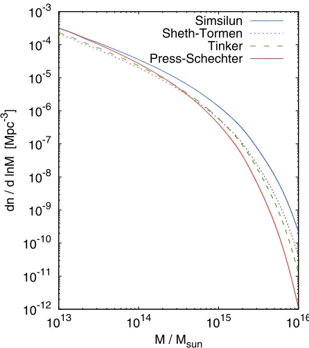
[image:3.612.62.285.401.652.2]Simsilun Sheth-Tormen Tinker Press-Schechter
FIG. 1. Mass function at the present-day instant: the upper blue line shows the mass function evaluated within the Simsilun simulation; the lower red line shows the Press-Schechter mass function; the dashed green line presents the Tinker mass function; the dotted purple line presents the Sheth-Tormen mass function.
10-20 10-18 10-16 10-14 10-12 10-10 10-8 10-6 10-4 10-2
1013 1014 1015 1016
z = 0
z = 1.0
z = 2.0
dn / d lnM [Mpc
-3 ]
M / Msun
[image:3.612.322.549.412.663.2]Simsilun Tinker
(where δ is the density contrast with respect to the back-ground density and Δ is the density contrast of the collapsed object). This condition can be fixed freely; e.g., for Figs. 1 and 2 we use Δ≈ ∞ (i.e., we stop just before the collapse is reached). This choice has been made to have a meaningful comparison with the Press-Schechter approach. However, for Figs.3and4we useΔ¼200with respect to the background critical density; this was done in order to have a meaningful comparison with the measure-ments obtained by the Atacama Cosmology Telescope. For Fig.5we useΔ¼200but with respect to the background matter density, which has been done in order to have a direct comparison with the results obtained by[18](cf. their Fig.1). Once the threshold is reached we stop the evolution. If we were to continue evolving past the threshold, then the region would have collapsed to a point. A typical timescale for Δ¼200, from passing the threshold to reaching the final stage of the collapse, is approximately 100 Myr.
Figure1shows the mass function obtained as described above. The mass function is evaluated at the present-day instant (i.e., z¼0). For comparison, the Tinker mass function is also presented. The procedure of evaluating the mass function is similar to the procedure implemented by Press and Schechter, where the evolution of over-densities and their collapse is modeled with a homogeneous top-hat model. In fact, if we setΣ¼0,W ¼0(which is equivalent to the FLRW evolution), and Δ¼1.69, we recover the Press-Schechter mass function, which is also presented in Fig.1.
This approach has several limitations: it does not include such effects as the baryonic feedback, cloud-in-cloud problem, and the scale-dependent bias [19]. In addition since the Press-Schechter procedure does not allow for halos to merge, the approach implemented within the Simsilun simulation also does not account for mergers. Thus, unlike in the real Universe, or as observed within theN-body simulations, small halos do not merge, which
105
106
107
108
109
1010
1011
0 0.2 0.4 0.6 0.8 1
455 deg2 full sky
Volume [M200c
= 1.77 ± 0.21
× 1015 Msun]
V [Mpc
3 ]
z
105
106
107
108
109
1010
1011
0 0.2 0.4 0.6 0.8 1
455 deg 2 full sky
Volume [M 200c
= 1.77 ± 0.21 × 10
15 Msun]
V [Mpc
3 ]
[image:4.612.321.556.44.387.2]z
FIG. 3. Volume covered by the full-sky and ACT-like surveys (solid red lines). For comparison the volumes needed to observe at least one object evaluated using the Simsilun (upper panel) and Tinker (lower panel) mass functions are also presented. The shaded region corresponds to the mass range of1.770.21× 1015 M⊙(the density thresholdΔis set to 200 with respect to the critical density, i.e.,M200c).
10-1
100
101
0 0.2 0.4 0.6 0.8 1
N
z
10-1
100
101
0 0.2 0.4 0.6 0.8 1
z=0.33 z=0.42 z=0.44 z=0.61 z=0.87
N=10.55 N=7.76 N=7.18
N=3.18
N=0.59
N
z
10-4
10-3
10-2
10-1
100
0 0.2 0.4 0.6 0.8 1
N
z
10-4
10-3
10-2
10-1
100
0 0.2 0.4 0.6 0.8 1
z=0.33 z=0.42 z=0.44 z=0.61 z=0.87
N=0.20 N=0.11 N=0.098 N=0.024
N=0.0015
N
z
[image:4.612.53.296.47.394.2]means that this procedure overestimates the number of objects at the lower end of the mass function. All of these effects are relevant for masses below1014 M⊙. Consequently one should not use the Simsilun simulation for reliable estimation of the mass function in this mass range. However, above a certain scale these effects become less relevant. The so-called“matter horizon”[20]is of order of 5 Mpc, i.e., a particle (be it a galaxy or an active galactic nuclei mass ejection) can only move up to a few Mpc within the age of a universe. A region of size 10 Mpc has approximately a mass
of1014M⊙and this is also the scale where the amplitude of the Press-Schechter mass function becomes smaller than the Tinker mass function (cf. Fig.1). Consequently, it is safe to assume that an object of mass beyond1015 M⊙ is created only by a collapse and mergers of smaller objects that are already within the a domain of influence of this object; i.e., it is not created by a merger of objects of masses∼1015 M⊙ (i.e., by objects that were separated in comoving coordinates by more than 10 Mpc). Therefore, the predictions based on the high-mass end of the mass function recovered with the Simsilun simulation should be considered as reliable.
III. THE MOST MASSIVE OBJECTS IN THE UNIVERSE
Assuming perfect completeness of a survey, the expected number of objects with masses between Mmin and Mmax detected in a survey of angular coverage dΩ and redshift rangezmin–zmaxcan be inferred directly from Eq.(9). There are two competing effects that contribute to the observed number of objects. The first one is the volume, i.e., the larger the redshift range, the larger the volume, and hence a larger number of expected objects. The second effect is related to the fact that the number density of the most massive objects decreases with redshift (cf. Fig.2), where the amplitude of the mass function is significantly lower at higher redshifts. These two competing effects are presented in Fig.3.
A. Most massive objects at high redshifts
Figure 3 shows the volume covered by the 455deg2 survey and full-sky survey (as a function of redshift). For comparison, the volume needed to observe one object with mass 1.770.21×1015 M⊙ (weighted average of the five most massive ACT clusters), at that redshift is also presented. The upper panel shows the results for the Simsilun mass function and the lower panel for the Tinker mass function. One should note that this is for comparison only, as these two volumes are not directly related. The volume covered by the survey is the volume within the past light cone; i.e., this is the volume which is evaluated across different times, from the present-daytðz¼0Þto a particu-lar redshifttðzÞ. In contrast, the volume needed to observe one object is the volume evaluated at a single time instant, i.e., this is the volume evaluated at that particular redshift. If the number density were constant and did not change with time, these two volumes would be directly comparable; i.e., if the volume covered by the survey were equal to the volume needed to observe one object at that redshift, then we would expect to see one object within the survey. However, since the number density decreases with redshift, thus when the volume covered by the survey is equal to the volume needed to observe one object at that redshift, we should expect to see at least one object (if not more). Consequently, if the volume covered by the survey is Tinker
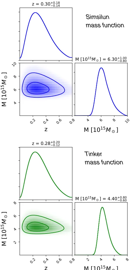
[image:5.612.64.285.46.504.2]mass function Simsilun mass function
always smaller than the volume needed to observe one object, then it is unlikely to expect to see any such objects in the survey.
As seen from Fig.3there are two regimes sensitive to the mass function. The first regime is the low-redshift Universe, where low volumes prevent observing most massive objects (since their number density is small, one requires a large volume to observe these rare objects). The second one is the high-redshift Universe where the most massive objects are not sufficiently evolved yet; conse-quently their very small number density makes them extremely rare, despite large volumes.
At high redshift the most effective method of detecting clusters is by the observations of the Sunyaev-Zel’dovich effect. However, this method does not allow us to estimate the mass of the observed cluster, and so one needs to implement other methods to estimate the mass. For the Atacama Cosmology Telescope (ACT) survey, the masses of the clusters (detected with the Sunyaev-Zel’dovich effect) were estimated using the scaling relations between the observed velocity dispersion and their mass. The five most massive clusters observed within the ACT survey are ACT-CL J0102-4915 at z¼0.87010.0009 with mass
M200c¼1.680.39×1015 M⊙; ACT-CL J0237-4939 at
z¼0.33440.0007 with mass M200c¼2.060.43×
1015 M
⊙; ACT-CL J0330-5227 at z¼0.44170.0008 with mass M200c ¼1.770.41×1015 M⊙; ACT-CL J0438-5419 at z¼0.42140.0009 with mass M200c¼ 2.180.52×1015 M⊙; and ACT-CL J0559-5249 at z¼ 0.60910.0014with mass M200c¼1.540.44×1015M⊙
[21]. The average uncertainty-weighted mass of these five clusters is1.770.21×1015 M⊙. As seen from Fig.3, for the Tinker mass function, these five most massive clusters are not expected to be seen within a455deg2survey; they are only expected to be observed within the full-sky survey. On the contrary, the Simsilun mass function does not have problems with explaining the existence of these objects; also their observed redshift range is in perfect agreement with predictions of the Simsilun simulation.
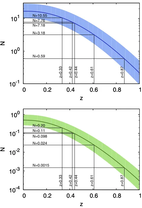
This discrepancy between the number of objects with masses1.770.21×1015 M⊙, expected to be observed in a455deg2 survey, is further presented in Fig.4. Figure4
shows the number of objects evaluated from Eq.(9) with
Mmin¼1.770.21×1015M⊙andzmin¼z. The redshift position and the expected numbers are also presented in Fig. 4, where the upper panel shows the results for the Simsilun mass function and the lower panel for the Tinker mass function. As seen from Fig.4, the Simsilun simulation with a slightly higher amplitude at the high-mass end of the mass function (compared to the Tinker mass function) has no problems with explaining the observed number of the most massive clusters observed by the ACT survey. On the other hand, the Tinker mass function seems to be at odds with the observed data.
B. Most massive objects at low redshifts
Apart from the high redshift, the second regime which is very sensitive to the prediction of the mass function is the number of the most massive objects at low redshifts, where the number of these objects is low due to small volumes. The larger the mass, the larger the volume is needed to observe such extreme objects. If the mass is too high, the probability of observing such objects goes to zero, and so there is an upper limit on the mass of the most massive objects. The predictions for the most massive objects obtained using the Simsilun and Tinker mass functions are presented in Fig.5. The most massive object is of the mass 6.3þ1.0
−0.8×10¹⁵ M⊙ for the Simsilun simulation, and 4.4−þ00..68×1015 M⊙ for the Tinker mass function.
If we were to compare these predictions with obser-vations, the most massive supercluster observed to date is most likely the Shapley Concentration, whose mass is estimated to be between 6×10¹⁵ M⊙ [22] and 8×10¹⁵ M⊙ [23], but likely even higher [24]. While the existence of such a massive object is in agreement with the Simsilun simulation, its existence is slightly at odds with the Tinker mass function.
However, if we take into account that the distance to the Shapley Concentration is approximately 200 Mpc, then the probability of observing such a massive object within such a small volume drops. The probability of observing an object with a mass of at least6×1015 M⊙ within the distance of 200 Mpc is3×10−2and3×10−3for Simsilun and Tinker mass functions, respectively. While this could be explained using the extreme value statistics, the prob-ability of observing two very massive objects within the distance of 200 Mpc is very low and poses a challenge for the standard cosmological model[25]. Indeed, for the Tinker mass function the probability of observing two objects with masses above 5×10¹⁵ M⊙ and within the distance of 200 Mpc is6×10−5, which makes it inconceiv-ably small. For the Simsilun mass function the probability of observing two objects with masses above5×1015 M⊙ and within the distance of 200 Mpc is3×10−3, which is still within3σ. Thus, taking into account the existence of the Great Attractor—distance between 50 and 80 Mpc and mass between4×1015M⊙and6×1015 M⊙[26]—it seems that again (as in the case of the ACT clusters) the predictions for the most massive objects obtained from the Tinker mass function are at odds with the data.
IV. CONCLUSIONS
FLRW models. Consequently, local properties differ from the global properties of the Universe. For example, overdense regions could be characterized by positive spatial curvature, which could affect the growth rate.
The approach implemented in this paper allows for cosmological properties of the Universe to vary. Consequently, the expansion rate or spacial curvature depends on the environment. Within this approach, we study the evolution of cosmic structures and focus on the formation of the most massive objects, i.e., objects with masses 1015 M⊙ and above. The obtained results suggest that the formation of these extremely massive objects proceeds faster within the Simsilun simulation compared to the standard approach.
We compare the results obtained within the Simsilun simulation to the predictions obtained using the Tinker mass function and test them against observational data. We find that the prediction for the number of the most massive objects obtained using the Tinker mass function is at odds with the observational data, whereas the Simsilun simulation correctly predicts the number of most massive ACT clusters, as well as the existence of the Shapley Concentration and the Great Attractor.
However, one should keep in mind that the Simsilun simulation does not allow for rotation or transfer of energy between various regions of the Universe, and thus, at sub-Mpc scales where these effects are important, the Simsilun simulation is not expected to work well. Therefore, more work is needed especially using more advanced schemes, such as the one based on the Lagrangian framework
[27–30]; the first application of this framework to obser-vationally realistic, standard N-body cosmological initial conditions was recently published in[31].
In summary, the results of this paper suggest that the formation of the most massive object could proceed in a slightly faster way than previously anticipated [18]. Our study was based on a simplified model, therefore, more investigation of this phenomenon is needed. If indeed the environment dependence of the growth rate of the most massive clusters is confirmed by more detailed study, then these effects will be of significance when analyzing the data from the next-generation satellite missions such as Euclid
[32]and eROSITA [33].
ACKNOWLEDGMENTS
K. B. acknowledges the support of the Australian Research Council through the Future Fellowship FT140101270. J. J. O. is supported by Lyon Institute of Origins (LIO) under Grant No. ANR-10-LABX-66 and by National Science Centre, Poland, under Grant No. 2014/13/ B/ST9/00845. This work is part of a project that has received funding from the European Research Council (ERC) under the European Union’s Horizon 2020 research and innovation program (ERC Advanced Grant No. 740021-ARTHUS, PI: T. Buchert). The corner plots were created using the software Corner [34]. Finally, discussions with and comments from Thomas Buchert, Boud Roukema, and David Wiltshire are gratefully acknowledged.
[1] S. Matarrese, O. Pantano, and D. Saez,Phys. Rev. D 47, 1311 (1993).
[2] S. Matarrese, O. Pantano, and D. Saez,Phys. Rev. Lett.72, 320 (1994).
[3] M. Bruni, S. Matarrese, and O. Pantano,Astrophys. J.445, 958 (1995).
[4] H. van Elst, C. Uggla, W. M. Lesame, G. F. R. Ellis, and R. Maartens,Classical Quantum Gravity14, 1151 (1997). [5] K. Bolejko,Classical Quantum Gravity35, 024003 (2018). [6] G. F. R. Ellis, Relativistic cosmology, in Proceedings of the International School of Physics “Enrico Fermi”, Course 47: General relativity and cosmology, edited by R. K. Sachs (Academic Press, New York and London, 1971), pp. 104–182.
[7] G. F. R. Ellis,Gen. Relativ. Gravit.41, 581 (2009). [8] R. Maartens, W. M. Lesame, and G. F. R. Ellis,Phys. Rev. D
55, 5219 (1997).
[9] R. A. Sussman and K. Bolejko,Classical Quantum Gravity
29, 065018 (2012).
[10] W. H. Press and P. Schechter, Astrophys. J. 187, 425 (1974).
[11] R. K. Sheth and G. Tormen,Mon. Not. R. Astron. Soc.329, 61 (2002).
[12] O. Lahav and Y. Suto,Living Rev. Relativity7, 8 (2004). [13] W. A. Watson, I. T. Iliev, A. D’Aloisio, A. Knebe, P. R. Shapiro, and G. Yepes,Mon. Not. R. Astron. Soc.433, 1230 (2013).
[14] S. G. Murray, C. Power, and A. S. G. Robotham, Astron. Comput.3, 23 (2013).
[15] J. Tinker, A. V. Kravtsov, A. Klypin, K. Abazajian, M. Warren, G. Yepes, S. Gottlöber, and D. E. Holz,Astrophys. J.688, 709 (2008).
[16] D. J. Eisenstein and W. Hu,Astrophys. J.496, 605 (1998). [17] P. A. R. Ade, N. Aghanim, M. Arnaud, M. Ashdown, J. Aumont, C. Baccigalupi, A. J. Banday, R. B. Barreiro, J. G. Bartlett et al. (Planck Collaboration), Astron. Astrophys.
594, A13 (2016).
[18] D. E. Holz and S. Perlmutter,Astrophys. J.755, L36 (2012). [19] V. Desjacques, D. Jeong, and F. Schmidt,Phys. Rep.733, 1
(2018).
[20] G. F. R. Ellis and W. R. Stoeger,Mon. Not. R. Astron. Soc.
[21] C. Sifón, F. Menanteau, M. Hasselfield, T. A. Marriage, J. P. Hughes, L. F. Barrientos, J. González, L. Infante, G. E. Addison, A. J. Baker et al., Astrophys. J. 772, 25 (2013).
[22] S. Bardelli, E. Zucca, G. Zamorani, L. Moscardini, and R. Scaramella,Mon. Not. R. Astron. Soc.312, 540 (2000). [23] C. J. Ragone, H. Muriel, D. Proust, A. Reisenegger, and H.
Quintana,Astron. Astrophys.445, 819 (2006).
[24] D. Proust, H. Quintana, E. R. Carrasco, A. Reisenegger, E. Slezak, H. Muriel, R. Dünner, L. Sodr´e, Jr., M. J. Drinkwater, Q. A. Parker et al., Astron. Astrophys. 447, 133 (2006).
[25] R. K. Sheth and A. Diaferio,Mon. Not. R. Astron. Soc.417, 2938 (2011).
[26] K. Bolejko and C. Hellaby,Gen. Relativ. Gravit.40, 1771 (2008).
[27] T. Buchert and M. Ostermann,Phys. Rev. D 86, 023520 (2012).
[28] T. Buchert, C. Nayet, and A. Wiegand,Phys. Rev. D87, 123503 (2013).
[29] A. Alles, T. Buchert, F. Al Roumi, and A. Wiegand,Phys. Rev. D 92, 023512 (2015).
[30] F. Al Roumi, T. Buchert, and A. Wiegand,Phys. Rev. D96, 123538 (2017).
[31] B. F. Roukema,Astron. Astrophys.610, A51 (2018). [32] L. Amendola, S. Appleby, D. Bacon, T. Baker, M. Baldi, N.
Bartolo, A. Blanchard, C. Bonvin, S. Borgani, E. Branchini et al.,Living Rev. Relativity16, 6 (2013).
[33] A. Merloni, P. Predehl, W. Becker, H. Böhringer, T. Boller, H. Brunner, M. Brusa, K. Dennerl, M. Freyberg, P. Friedrich et al.,arXiv:1209.3114.