doi: 10.3389/fmars.2019.00444
Edited by:
Fei Chai, State Oceanic Administration, China
Reviewed by:
Arthur J. Miller, University of California, San Diego, United States Lei Zhou, Shanghai Jiao Tong University, China
*Correspondence:
Detlef Stammer [email protected] Annalisa Bracco [email protected]
Specialty section:
This article was submitted to Ocean Observation, a section of the journal Frontiers in Marine Science
Received:18 November 2018
Accepted:05 July 2019
Published:31 July 2019
Citation:
Stammer D, Bracco A, AchutaRao K, Beal L, Bindoff NL, Braconnot P, Cai W, Chen D, Collins M, Danabasoglu G, Dewitte B, Farneti R, Fox-Kemper B, Fyfe J, Griffies SM, Jayne SR, Lazar A, Lengaigne M, Lin X, Marsland S, Minobe S, Monteiro PMS, Robinson W, Roxy MK, Rykaczewski RR, Speich S, Smith IJ, Solomon A, Storto A, Takahashi K, Toniazzo T and Vialard J (2019) Ocean Climate Observing Requirements in Support of Climate Research and Climate Information. Front. Mar. Sci. 6:444. doi: 10.3389/fmars.2019.00444
Ocean Climate Observing
Requirements in Support of Climate
Research and Climate Information
Detlef Stammer1* , Annalisa Bracco2* , Krishna AchutaRao3, Lisa Beal4,
Nathaniel L. Bindoff5,6, Pascale Braconnot7, Wenju Cai8, Dake Chen9, Matthew Collins10,
Gokhan Danabasoglu11, Boris Dewitte12,13,14,15, Riccardo Farneti16, Baylor Fox-Kemper17,
John Fyfe18, Stephen M. Griffies19, Steven R. Jayne20, Alban Lazar21,
Matthieu Lengaigne22, Xiaopei Lin23,24, Simon Marsland25, Shoshiro Minobe26,
Pedro M. S. Monteiro27, Walter Robinson28, Mathew Koll Roxy29, Ryan R. Rykaczewski30,
Sabrina Speich31, Inga J. Smith32, Amy Solomon33, Andrea Storto34, Ken Takahashi35,
Thomas Toniazzo36and Jerome Vialard37
1Center für Erdsystemforschung und Nachhaltigkeit, Universität Hamburg, Hamburg, Germany,2School of Earth and Atmospheric Sciences, Georgia Institute of Technology, Atlanta, GA, United States,3Centre for Atmospheric Sciences, Indian Institute of Technology Delhi, New Delhi, India,4Rosenstiel School of Marine and Atmospheric Science, University of Miami, Miami, FL, United States,5Institute for Marine and Antarctic Studies, University of Tasmania, Hobart, TAS, Australia,6CSIRO Oceans and Atmospheres, Hobart, TAS, Australia,7Laboratoire des Sciences du Climat et
de l’Environnement, Unité Mixte CEA-CNRS-UVSQ, Université Paris Saclay, Gif-sur-Yvette, France,8Centre for Southern Hemisphere Oceans Research, CSIRO, Aspendale, VIC, Australia,9State Key Laboratory of Satellite Ocean Environment Dynamics, Second Institute of Oceanography, State Oceanic Administration, Hangzhou, China,10College of Engineering, Mathematics and Physical Sciences, University of Exeter, Exeter, United Kingdom,11Climate and Global Dynamics Laboratory, National Center for Atmospheric Research, Boulder, CO, United States,12Centro de Estudios Avanzados en Zonas Áridas, Coquimbo, Chile,13Departamento de Biología, Facultad de Ciencias del Mar, Universidad Católica del Norte, Coquimbo, Chile,14Millennium Nucleus for Ecology and Sustainable Management of Oceanic Islands (ESMOI), Coquimbo, Chile,15LEGOS, Université de Toulouse, IRD, CNES, CNRS, UPS, Toulouse, France,16Earth System Physics Section, Abdus Salam International Centre for Theoretical Physics, Trieste, Italy,17Department of Earth, Environmental, and Planetary Sciences, Brown University, Providence, RI, United States,18Canadian Centre of Climate Modelling and Analysis, Environment and Climate Change Canada, Victroia, BC, Canada,19NOAA Geophysical Fluid Dynamics Laboratory, Princeton, NJ, United States,20Department of Physical Oceanography, Woods Hole Oceanographic Institution, Woods Hole, MA, United States,21CNRS, IRD, MNHN, Laboratoire d’Océanographie et du Climat: Expérimentations et Approches Numériques, Sorbonne Université, Paris, France,22Laboratory of Oceanography and Climate: Experiments and Numerical Approaches, Institute of Research for Development, Paris, France,23Physical Oceanography Laboratory, Institute for Advanced Ocean Studies, Ocean University of China, Qingdao, China,24Qingdao National Laboratory for Marine Science and Technology, Qingdao, China,25CSIRO Climate Science Centre, Canberra, ACT, Australia,26Department of Earth and Planetary Sciences, Faculty of Science, Hokkaido University, Sapporo, Japan,27Southern Ocean Carbon – Climate Observatory, CSIR, Cape Town, South Africa,28Department of Marine, Earth, and Atmospheric Sciences, North Carolina State University, Raleigh, NC, United States,29Centre for Climate Change Research, Indian Institute of Tropical Meteorology, Pune, India,30School of the Earth, Ocean, and Environment, University of South Carolina, Columbia, SC, United States, 31UMR8539, IPSL, ENS – PSL, Laboratoire de Météorologie Dynamique, Paris, France,32Department of Physics, University of Otago, Dunedin, New Zealand,33Earth System Research Laboratory, National Oceanic and Atmospheric Administration, Cooperative Institute for Research in Environmental Sciences, University of Colorado, Boulder, Boulder, CO, United States, 34Centre for Maritime Research and Experimentation, La Spezia, Italy,35Servicio Nacional de Meteorología e Hidrología del Perú, Instituto Geofisico del Peru, Lima, Peru,36Bjerknes Centre for Climate Research, University of Bergen, Bergen, Norway,37IRD, IPSL, CNRS, IRD, MNHN, LOCEAN Laboratory, Sorbonne University, Paris, France
lower boundary to the atmosphere, driving, and modifying atmospheric weather. Understanding and monitoring ocean climate variability and change, to constrain and initialize models as well as identify model biases for improved climate hindcasting and prediction, requires a scale-sensitive, and long-term observing system. A climate observing system has requirements that significantly differ from, and sometimes are orthogonal to, those of other applications. In general terms, they can be summarized by the simultaneous need for both large spatial and long temporal coverage, and by the accuracy and stability required for detecting the local climate signals. This paper reviews the requirements of a climate observing system in terms of space and time scales, and revisits the question of which parameters such a system should encompass to meet future strategic goals of the World Climate Research Program (WCRP), with emphasis on ocean and sea-ice covered areas. It considers global as well as regional aspects that should be accounted for in designing observing systems in individual basins. Furthermore, the paper discusses which data-driven products are required to meet WCRP research and modeling needs, and ways to obtain them through data synthesis and assimilation approaches. Finally, it addresses the need for scientific capacity building and international collaboration in support of the collection of high-quality measurements over the large spatial scales and long time-scales required for climate research, bridging the scientific rational to the required resources for implementation.
Keywords: ocean observing system, ocean climate, earth observations, in situ measurements, satellite observations, ocean modeling, climate information
INTRODUCTION
The ocean is an integral part of the climate system: understanding how climate change and variability have shaped it and how climate will be influenced by future changes is a major societal challenge. Key to understanding the ocean’s role in the Earth’s climate system is monitoring changes in the ocean circulation, heat and carbon content, freshwater, biogeochemistry and sea level, as well as studying the interactions of the ocean with the atmosphere, cryosphere, land, and ecosystems. In addition, a firm knowledge of the changing physical environment is fundamental to understanding the ocean’s biogeochemistry and ecosystem functioning, variability, and change. Obtaining high-quality ocean climate observations on a sustained basis is also key to attributing the observed changes of the ocean state and therefore obtaining reliable climate predictions for a range of applications and users (Clivar, 2018 Science Plan1).
Through OceanObs’99 (Koblinsky and Smith, 2001) and OceanObs’09 (Hall et al., 2010) and through a continuous discussion of the global climate observing system (GCOS) implementation strategy2, the design of the ocean observing
system has emerged. It consisted, initially, in a definition of essential climate variables (ECVs) and their sampling characteristics in the ocean and elsewhere, and has evolved from a platform-centric perspective to an integrated cross-platform,
1
http://www.clivar.org/news/clivar-released-second-generation-science-plan-and-implementation-strategy
2https://unfccc.int/sites/default/files/gcos_ip_10oct2016.pdf
parameter-centric observing system. The challenge now is for the climate-oriented observing system to evolve further into one serving the increasing needs for ocean climate information at refined spatial and temporal scales, particularly in the face of advancing anthropogenic climate forcing.
In this whitepaper we review in section “Observing Requirements for Climate” the observing requirements for major processes of climate interest organized around global considerations and basins-specific aspects with an emphasis on the open ocean. Challenges and opportunities for the ocean margins are discussed in section “Observing Requirements for Bounday Currents and Continental Margins,” while needs specific to climate modeling, forecasting and to synthesis and reanalysis efforts are presented in section “Ocean Observations for Climate Modeling and Climate Information,” followed by concluding remarks in section “Summary and Final Remarks.”
OBSERVING REQUIREMENTS FOR
CLIMATE
currents and mixing, and feed back into the atmosphere and the cryosphere. Many processes and mechanisms contribute to this redistribution over a wide range of scales in space and time. Understanding and monitoring them is needed to quantify ocean climate variability and change, as well as to constrain and initialize climate models and remedy model biases for improved hindcasting and prediction.
An ocean observing system for climate needs to provide essential information on a sustained long-term basis for monitoring, understanding, and forecasting within all ocean basins (The National Academies of Sciences, Engineering, and Medicine [NASEM], 2017). Specifically, its components should cover climate-observing parameters concerned with changes of the ocean circulation and its budgets of heat, freshwater, carbon, and nutrients, and the exchanges of heat, momentum, freshwater, and gases between the ocean, atmosphere, land, and cryosphere. Parameters concerned with sea level as an integral indicator for climate change (see alsoPonte et al., 2019) should also be included. Several of the observing requirements are general in nature and concern the global ocean domain; others concern regional specificities and are presented separately in each ocean basin.
General Considerations Concerning the
Global Ocean Domain
General observing requirements involve sustained in situ and space-based approaches that sample essential climate parameters over a broad range of spatial and time scales, as outlined in the GCOS implementation plan. Space-based measurements cover globally the surface expression of a broad spectrum of ocean processes. In contrast,in situmeasurements provide the full-depth resolution required to monitor the vertical structure of climate changes in the ocean. They are also essential to climate-quality satellite data for calibration and inter-calibration purposes. The combination ofin situand space measurements is indispensable in regional and global process studies and estimates of anthropogenic heat and carbon uptake, among others (e.g.,
Palmer et al., 2019;Wannikhov et al., 2019).
Space-based climate monitoring requirements involve sustained satellite measurements of sea surface temperature (SST) (O’Carroll et al., 2019), surface wind and wind stress (Cronin et al., 2019), sea surface height (SSH) from which surface geostrophic currents can be derived and gravity changes (mass changes in the climate system), surface fluxes of heat (Cronin et al., 2019) and freshwater including rainfall, sea surface salinity (SSS), surface waves (Villas Boas et al., 2019) and ocean color. They should be sampled at least twice daily, ideally four times a day, and at a spatial scale that resolves accurately the ocean mesoscale [O(1) km]. Technology developments, such as new sensors and satellite constellations, are key to improve and expand these measurements. One priority is pursuing the development of wide-swath altimeters to measure meso- and submeso-scale SSH variations in crucial energetic regions.
It is imperative to sustain these observations (satellite or
in situ) over a long period with climate-quality stability and
precision. This requirement is all the more important if the
physical signal deviates from a Gaussian distribution, since in that case the statistical moment of the time series may not be stable in time, reflecting the occurrence of extreme events. Global budgets of ECVs, such as heat, freshwater, and carbon rely on top-to-bottom in situ measurements using various platforms. A global full-water column Argo float array (Claustre et al., 2019) and high-quality ship-based CTD sections are therefore mandatory, and should include measurements under sea ice. Equally important is the monitoring of boundary currents through systems that continuously measure their transport – a recommendation formulated during OceanObs’09 but never implemented.
In situ measurements of the above variables are currently
coordinated by the global ocean observing system (GOOS) and collected through the global tropical moored buoy arrays, Argo and global drifter programs, high resolution XBT transects, and Go-SHIP surveys.
The surface drifter array provides a Lagrangian view of ocean circulation, as well as surface temperature, and a growing number of barometric pressure measurements essential to weather forecasting. Argo profiling floats sample temperature, salinity, and derived geostrophic currents more or less homogeneously throughout the ocean subsurface, except in the polar regions, and sparsely below 2000 m depth (Roemmich et al., 2015).
During OceanObs’09 the expansion to routinely include biogeochemical parameters, such as O2, carbon, pH and nutrients, was recommended. BioArgo floats, while still low in number, are being implemented, contributing oxygen profiles and, in some cases, additional biogeochemical variables. Improving globally the spatial and temporal coverage of subsurface measures of biogeochemical tracers collocated with physical measurements is even more critical today with accelerating acidification, oxygen depletion, and ecosystem change. New Deep-Argo technology is also coming on line to increase observations below 2000 m.
Surface and subsurface mooring arrays augment these observations, primarily along the equator and in critical boundary regions, with high temporal and/or spatial resolution observations of surface fluxes and subsurface T, S, currents, and at times oxygen, nutrients, and fluorescence. Moorings require routine maintenance and hence datasets are often short with respect to the climate signals of interest. Basin-wide GO-SHIP transects are essential to provide full depth observations of climate variables, including a full suite of biogeochemical parameters that can only be measured through water collection. Paleoclimate proxy data, such as through ocean sedimentary cores and corals, provide critical extensions of the instrumental record.
Since changes in mass and heat content drive sea level changes, regionally and globally, their monitoring over the full water column and under sea ice is essential. These measurements, in combination with sustained altimetry and tide gauge data, form the basis for studies of sea level change, and its coastal impacts (a WCRP Grand Challenge).
water isotope retrievals, as well as benchmarks for isotope-equipped climate model simulations of the global water cycle (also a WCRP Grand Challenge), as they intersect with clouds, circulation, and climate.
The Atlantic Ocean
Background
The Atlantic Ocean, through its Meridional Overturning Circulation (AMOC; Frajka-Williams et al., 2019), plays a unique role in the Earth’s climate. Different from the vertical overturning circulation in the other basins, the AMOC carries warm saline water from the South Atlantic northward in the upper 1200 m (deemed as the “upper limb”) that is then transformed into the North Atlantic deep water (NADW) in the subpolar North Atlantic and Nordic Seas, and returned southward in the “lower limb” (1200–4000 m). This circulation is far more complex than commonly portrayed and involves the whole water column, linking the upper, mode, intermediate, deep and bottom waters formed and transformed in this ocean, or imported from other basins. The AMOC influences the northward transport of heat (Bryden and Imawaki, 2001) and its release to the atmosphere, providing a significant fraction of the zonally integrated atmospheric energy flux northward of 30◦
N (Rhines et al., 2008). Additionally, it captures about 30% of the anthropogenic excess of heat (Häkkinen et al., 2015;Palmer et al., 2017) and carbon (Takahashi et al., 2009). It drives the inter-basin transport of freshwater, nutrients, carbon, oxygen and other biogeochemical quantities (Tagklis et al., 2017), impacts the marine ecosystem, and affects the global hydrological cycle, with a clear connection to predictability, from seasonal to decadal (Schlundt et al., 2014;Fu et al., 2018).
The AMOC is thought to be a driver of Atlantic multi-decadal variability (AMV), whose sub-polar center of action is linked to ocean dynamics (Kerr, 2000). The AMV, in turn, impacts Sahel rainfall, North American and European weather, the South and East Asian Monsoons, and Arctic sea ice (Sutton and Hodson, 2005). Decadal AMOC variability is positively correlated with northward energy transport in the ocean, but anti-correlated with transport in the tropical atmosphere; regional dynamical feedbacks, however, are unknown. Atmosphere-ocean interactions have been extensively studied on interannual time scales, but are less understood at decadal scales. The spatial dynamical scales involved in the variability and change of the Atlantic Ocean are small, as all current systems of interest are significantly affected by fronts and eddies at the mesoscales (10–300 km).
Atlantic Observing Requirements
The scientific community is moving toward a better rationalization of the Atlantic Observing System as a whole (AtlantOS, deYoung et al., 2019). Being the ocean that receives a large portion of the oceanic excess heat uptake, and that hosts major modes of climate variability, the Atlantic should be observed adequately to accompany the society in adaptation to sea level rise (Ponte et al., 2019), ocean warming (Palmer et al., 2019), ocean acidification (Tilbrook et al., 2019), and the increased intensity of extreme events, including
hurricanes (Goni et al., 2019). It is necessary to improve process understanding (in particular, ocean interactions between the meso- and submeso-scales and the large-scale circulation, air-sea interactions at the meso- and submeso-scales, and heat, freshwater, oxygen and carbon uptake, transport and release to the atmosphere), monitor changes, and feed robustly model developments (Fox-Kemper et al., 2019; Subramanian et al., 2019) and predictions (Penny et al., 2019).
Because of the particular nature of the Atlantic Ocean circulation, observations of currents, salinity, and temperature fields are needed from the surface to the ocean floor. These variables are also mandatory to monitor climate change and enable robust numerical weather prediction, as well as intraseasonal to interdecadal forecasts. However, because of the different scales of variability, they could be sampled with reduced spatial and temporal resolution for depths greater than 2000 m.
The current Atlantic basin observing system (schematized in
Figure 1) is composed of AMOC (Frajka-Williams et al., 2019) and Tropical Atlantic PIRATA mooring arrays (Foltz et al., 2018). The AMOC array covers the full depth of the water column near the continental slope; the PIRATA array is limited to the upper ocean but includes heat and momentum flux observations. An assessment on the evolution of the tropical atlantic observing system (TAOS) to expand and rationalize observations in this region is ongoing (Johns et al., 2018;Foltz et al., 2019).
[image:4.595.304.551.430.640.2]In the open-ocean upper 1500–2000 m, the core Argo program is well developed in the North Atlantic, but more sparse in the tropical, and even more so in the South Atlantic. In the North Atlantic, deployments of BGC Argo and Deep Argo have been
initiated but remain in an early development and coverage stage (Roemmich et al., 2019).
The Atlantic basin is regularly (on a 5–10 years base) surveyed by repeated GO-SHIP cruises (Sloyan et al., 2019), and other cruises servicing the various deep moorings and mooring arrays as well as oceanographic cruises organized by finite-time lifespan research projects. These cruises are essentials in providing regular sampling of physical and biogeochemical properties over the full ocean depth not attainable by the Argo core floats nor by the mooring arrays alone.
The ship of opportunity program (SOOP) acquires measurements from volunteer merchant ships that regularly undertake shipping routes crossing the basin. This program helps to increase thein situsampling of the surface ocean (temperature and salinity via thermosalinographs instrument mounted close to the water intake of the vessel) and the upper 700 m of the ocean temperature (mainly) by a high resolution (every 10–35 km) deployment of expendable bathymographs (XBTs).
A dense array of buoys drogued at 15 m of depth that measure SST, surface currents and barometric pressure, via the global drifter program (GDP), is also maintained across the basin, mostly through the ship-volunteering program (Lumpkin et al., 2017).
Ocean underwater gliders deployment has been occurring along and near the North American continental slope within the global ocean gliders program (Testor et al., 2019). Typically, gliders profile from the surface to the bottom (over the continental shelf), or to 200–1000 m depth in the open ocean. However, their spatial coverage remains marginal compared to the extent of the Atlantic slope boundary. Indeed, sustained projects in the Atlantic include only observations in limited spots of the western, eastern and northern boundaries of the North Atlantic (Testor et al., 2019).
Observations should be enhanced in key regions related to the AMOC (the Labrador and Irminger Seas and the North Atlantic passages overflows, the South Atlantic that interconnects actively the North Atlantic with the rest of the world ocean) ( Frajka-Williams et al., 2019), in the Tropical Atlantic that plays an important control on weather extremes and climate modes (Foltz et al., 2019; Goni et al., 2019), and in the eastern and western boundary current systems (BCs) that are currently not sampled by the core Argo floats program, nor fully covered by the various Atlantic mooring arrays (Todd et al., 2019). Indeed, BCs not only regulate the meridional heat and fresh-water transports and cloud formation, but strongly influence atmosphere dynamics (Small et al., 2014;O’Reilly et al., 2017) and decadal variability (Gulev et al., 2013).
We recommend the continuation of all observing systems currently in place (core Argo and BGC Argo, AMOC, and PIRATA arrays, GO-SHIP cruises, surface drifters, VOS), and the enhancement of surface observations and observations in the atmosphere beyond current practices. In addition, we recommend enhancing subsurface ECV observations, as well as adding variables such as oxygen and pH, by maintaining and expanding the sensors equipping mooring arrays and observations undertaken by ships, and by implementing Deep Argo and BGC Argo.
The Pacific Ocean
Background
The Pacific Ocean is the largest of the world’s oceans and hosts the strongest interannual tropical climate mode, the El Niño Southern oscillation (ENSO), an ocean–atmosphere coupled phenomenon (Timmermann et al., 2018). ENSO exhibits huge worldwide socio-economical and environmental impacts (McPhaden et al., 2006). The Pacific basin accounts for much of the interannual variability of precipitation and tropical cyclones, inducing an elevated risk of drought in the western part of the basin and of flooding on the eastern side that cause widespread ecosystems disruptions, including severe bleaching of corals. Because of its remote influence through atmospheric teleconnections, ENSO also impacts the Indian and Atlantic oceans (Klein et al., 1999), and is in turn impacted by both (Kucharski et al., 2011;Terray et al., 2016).
At decadal to multidecadal timescales, the interdecadal Pacific oscillation (IPO), driven partly by decadal ENSO modulations (Power et al., 1999), is a major source for low-frequency climate variations, worldwide. The IPO affects the weather and climate in many regions of the globe (Dong and Dai, 2015), drives important state transitions observed in marine ecosystems across the Pacific Ocean (Mantua et al., 1997), and has been hypothesized as major cause of the recent slowdown in global surface warming (Kosaka and Xie, 2013). The observed warming trend in the past century has a complicated structure in the Pacific, with ‘hot spots’ along the western boundary currents (Wu et al., 2012). There are large uncertainties about the nature of this trend, calling for the need of sustained and un-interrupted monitoring, also with respect to its likely impacts on phytoplankton growth (Marinov et al., 2010).
The eastern tropical Pacific Ocean hosts two of the four largest oxygen minimum zones (OMZ) in the world, located to the north and the south of the equator. Significant global deoxygenation together with expansion of the OMZ in the tropical Pacific has been observed over the past 50 years (Stramma et al., 2008). This expansion will result in the transition, adaptation, and/or extinction of different marine species in the tropical Pacific Ocean (Breitburg et al., 2018).
Understanding and projecting climate changes induced by anthropogenic forcing in this region, including changes in background state and ENSO characteristics (Cai et al., 2015), are critical for assessing future socioeconomic and environmental impacts, as well as planning adaptation strategies. The latter are especially important for the highly populated coastal regions, including the Pacific island communities that are vulnerable to climate change through sea level rise, ocean acidification, and changes in storms characteristics.
Pacific Observing Requirements
systems, including the Indonesian throughflow (ITF) to the Indian Ocean. Because of the key role of the Pacific Ocean on global Earth’s climate, it is also necessary to observe ocean surface wind stress and heat fluxes in the tropical Pacific at hourly intervals. Momentum and heat fluxes are essential for inter-calibrating satellite missions, driving ocean models and ocean reanalysis products, detecting ENSO precursors, and assessing and understanding tropical Pacific climate variations and climate change.
In the BCs of the Pacific heat and freshwater fluxes should be monitored through hourly observations of temperature, salinity, and velocity over the ocean’s depth. These highly variables currents are indeed vital for predicting climate changes, for ENSO forecast and decadal prediction. Spatial and temporal coverage of subsurface measurements of oxygen, nutrients, chlorophyll, and pH should also be improved.
The parameters above could be observed by adding the necessary sensors to the existing Tropical Pacific Moored Array, which is a key component of the broader observing system. Eventual replacement of moorings with other observing technologies are being considered3and should be done carefully,
to ensure continuity of the climate records, e.g., with an overlap of the existing and new observing platforms over a sufficiently long time to allow a thorough examination of any consequences of the platform change. The existing Tropical Pacific Moored Array should be enhanced with additional direct surface flux measurements and biogeochemical and bio-optical sensors (pCO2, chlorophyll concentration, particulate backscatter, oxygen, and nutrients). Furthermore, we recommend incorporating water isotope sampling/analysis on ships, including those servicing the Tropical Pacific Moored Array, as well as prioritizing island-based collection of rainwater, seawater, and vapor water isotopes wherever feasible, and deploying Argo floats with biogeochemical and bio-optical sensors, particularly in equatorial Pacific upwelling and OMZs regions. The current observing system, reviewed in this issue by Smith et al. (2019), would also benefit from an enhanced regional coordination in the far Eastern tropical Pacific where no mooring is currently available within the Tropical Pacific Moored Array albeit being the location of extreme El Nino development.
In general terms, we support developing a multi-platform approach for monitoring velocity, temperature, salinity, and biogeochemistry in the boundary currents of both the northern and southern hemispheres. This holds especially for the Pacific Ocean, building on the CLIVAR endorsed North Pacific Ocean circulation experiment (NPOCE) and the Southwest Pacific Ocean and climate experiment (SPICE). Finally, seasonal to interannual changes in the upper ITF that links the Pacific to the Indian Ocean should be monitored through direct observations and development of proxies for temperature, salinity, and velocity down to sill depths at hourly intervals. This can be achieved through enhancement of the IX1 XBT line with additional Argo floats and a pilot glider program, and maintaining multi-year mooring arrays to measure the full depth ITF of the major
3http://tpos2020.org/
inflow (e.g., Makassar, Maluku, and Halmahera) and outflow (e.g., Lombok, Ombai, and Timor) passages.
The Indian Ocean
Background
Although the Indian Ocean is the smallest of the world’s oceans, it has accounted for more than 50% of global ocean heat gain over the last decade (Vialard, 2015; Desbruyères et al., 2017) and harbors two of the most severe OMZs (Paulmier and Ruiz-Pino, 2009). Indian Ocean rim countries are home to almost one third of the global population. Many depend on fisheries and agriculture and have poor adaptive capacity, making them especially vulnerable to changes in ocean climate, including declines in fish catch, intensification of tropical cyclone intensity, increased drought (Roxy et al., 2015), and sea level rise. For instance, the Bay of Bengal accounts for 5% of tropical cyclones globally, but 80% of the associated fatalities (Paul, 2009).
The unique circulation and stratification of the Indian Ocean (Schott et al., 2009), driven by reversing monsoon winds, an influx of tropical waters from the Indonesian Seas, and massive run-off from the Asian continent, enhance important coupled modes of variability, such as the Madden-Julian oscillation (MJO) (Zhang, 2005), the monsoon intra-seasonal oscillation (MISO), and the Indian Ocean dipole (Webster et al., 1999), that have far-reaching impacts on rainfall, cyclogenesis, and ENSO. The recent rapid warming in the Indian Ocean has been attributed to an increasing trend in the ITF (Lee et al., 2015; Hu and Sprintall, 2017; Zhang et al., 2018) and an intensified Walker Circulation. Yet long-term variability in the ITF and in other dominant flux components of the basin-wide heat budget, e.g., the Agulhas Current (Bryden and Beal, 2001) or the upper-ocean overturning (Talley et al., 2003), remains poorly constrained. Modes of decadal variability also remain largely unknown in the Indian Ocean (Han et al., 2014), where the observing system dates back only 10 years.
The tropical Indian Ocean has a large warm pool (surface temperature >27.5◦
C), linked to the Pacific, that has a global reach, driving atmospheric convection, and the Walker Circulation. The warm pool, together with the thermocline ridge of the western tropical gyre, is strongly coupled with the atmosphere at intraseasonal timescales (MJO and MISO,Vialard et al., 2009; DeMott et al., 2015). Observing and simulating correctly these climate modes could improve monsoon forecasting and seasonal climate predictability throughout the tropics, yet measurements of upper ocean variability and surface fluxes have long been precluded in the western tropical Indian Ocean owing to piracy, while to the east, near the ITF exit, disagreements between flux products remain.
oxide, a greenhouse gas with almost 300 times the potency of CO2 (Naqvi et al., 2010). Observations of biogeochemical parameters to monitor subsurface expansion and impacts of these OMZs are lacking, and satellite ocean color proxies for tracking primary productivity have not been validated in this basin.
Indian Ocean Observing Requirements
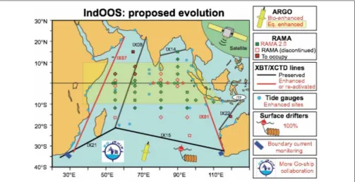
The existing Indian Ocean sustainable observing system (IndOOS) is being reviewed under the leadership of the CLIVAR-IOC GOOS Indian Ocean Region Panel4. This review established
that the current IndOOS system (seeFigure 2for its components) resolves reasonably the equatorial variability associated with the MJO and MISO, monsoon circulation and Indian Ocean Dipole. Key phenomena or regions that require enhanced observations are the heat and freshwater transport of the ITF, Agulhas and Leeuwin BCs, air-sea fluxes, and the Arabian Sea including biogeochemical aspects such as its OMZ. Variability in the ITF could be captured through enhancement of the IX1 XBT line with additional Argo floats, a pilot glider program, and exploration of the use of tomography for monitoring heat transport in the main passages of Lombok, Ombai, and Timor. Monitoring the subtropical boundary currents can be achieved with a mixture of tall moorings, CPIES, and glider programs. Pilot hydrographic end-point moorings as part of these arrays, in waters 2000 m deep or more, will allow a better handle on the basin-scale variations in oceanic heat content. In the tropics, the RAMA (Research Moored Array for African-Asian-Australian Monsoon Analysis and Prediction) tropical observing system should be expanded westward into the Arabian Sea (now that piracy is resolved) and enhanced with more direct flux measurements and a new surface flux reference site northwest of Australia. Finally, Argo floats with biogeochemical and bio-optical sensors should be deployed throughout the Indian Ocean, particularly in the Arabian Sea upwelling and OMZ regions and in the Bay of Bengal. An overview of the IO observing system requirements is given inFigure 2.
Polar Oceans
Background
The northern and southern polar oceans, present distinct, and at times shared, observational challenges and opportunities. The unique environment and the presence of sea ice complicate obtaining continuous, systematic observations, while promoting the development of new technology, and observational platforms. Polar oceans have experienced significant changes in heat/freshwater sources and fluxes from lower latitudes, sea ice melt, and river runoff. However, since the 1970s the decrease in Arctic sea ice cover has been widespread and dramatic (Vaughan et al., 2013), whereas Antarctic sea ice area changes have been strongly regional, with both increases and decreases ( Richter-Menge and Mathis, 2017; Stammerjohn and Scambos, 2017). More recently, polar amplification, where the polar region warms to higher temperatures and more rapidly than lower latitudes, has become of major concern in the northern hemisphere, but is not (yet) realized in the Southern Ocean (Lind et al., 2018).
4http://www.clivar.org/indoos-review-2006-2016
The Arctic Ocean plays a key role in the global overturning circulation and is a nexus of Atlantic Ocean variability, Pacific Ocean variability, and coastal environments, with run-off from ice sheets and large rivers being critical to ocean properties and circulation. A number of hypotheses for Arctic climate variability have been proposed but cannot be confirmed with current measurements. For example, how Atlantic water enters the Arctic, how it is redistributed within the Arctic interior, or the balance of forces that control the net outflow through the Canadian Arctic Archipelago. This complex system requires an integrated observational network to monitor and characterize sources and sinks of heat and salt into and out of the Arctic, and their changes. Direct observations of these sources are lacking, as in the case of fresh water inputs due to ice shelf basal melt and iceberg calving. However, in the broader region of the Arctic Mediterranean (Nordic Seas and Arctic Ocean), current meter arrays have been in operation at critical gateways or “choke points,” such as the Bering Strait and across the Greenland-Scotland Ridge, since the 1990s, providing monthly, if partly intermittent, time-series (e.g., Bringedal et al., 2018). Arrays operate also at key sections within the region, e.g., Svinøy Section, Barents Opening, and in the Fram Strait (Dickson et al., 2008), and in Davis Strait (Curry et al., 2014).
The Southern Ocean connects the Atlantic, Pacific, and Indian Oceans and, as explained in more detail inNewman et al., 2019, has a major impact on climate change signals. Recent estimates show that Southern Ocean circulation changes may account for 75% of the total excess heat linked to the airborne fraction of anthropogenic CO2and 50% of the anthropogenic CO2taken up by the ocean (Frölicher et al., 2015).
Decadal variability in heat and CO2storage in the “upper” and “lower” loops of the MOC in the Southern Ocean may modulate both anthropogenic and natural CO2 reservoirs (Gruber et al.,
2019). The Southern Ocean also plays a critical role in the ventilation of the low latitude ocean interior through mid-and deep-water masses. Freshening mid-and volume decrease of the heaviest water mass in the world’s ocean, the Antarctic bottom water (AABW), are the two strongest decadal signals ever observed in the deep oceans (Rintoul, 2018). AABW is a mixture of high salinity brine rejected in coastal polynyas during ice formation and surrounding circumpolar deep water, but the mixing process has not been observed directly, and links between surface forcing and AABW remain speculative. These factors, combined with the seasonal variability in sea ice, intense meso-and submesoscale features meso-and extreme synoptic scale winds, pose a challenge to resolving the seasonal to decadal variability in the storage, and ventilations through sustained observations.
High-Latitude Observing Requirements
FIGURE 2 |IndOOS original design and current state. The original IndOOS design comprises the RAMA, Argo, XBT/XCTD, surface drifting buoys and tide gauges components.
bottom pressure. However,in situmeasurements of these remote sensing products are rare, making calibration and validation of satellite algorithms challenging.
Free-drifting profiling floats present challenges in the polar oceans due to the likelihood of being trapped under ice and damaged. Technology developments allow the floats to sense the ice presence and store data for a number of years, but failure rates remain high. Efforts are underway to improve this problem. New technologies are being tested, such as the NOAA autonomous sailing drone that measures the near-surface ocean and atmosphere environments, and a system of moored sound sources maintained by the Alfred Wegener Institute in the Weddell Sea.
In the Arctic, well constrained transport estimates of volume, heat, and salt/freshwater in and out of the basin exist. It is imperative to maintain such gateway observations at a time when the climate system is in flux. However, key branches of the circulation and exchange, e.g., the Arctic circumpolar boundary current (ACBD), remain mostly unobserved. Significant work has been done to characterize freshwater storage within the Arctic Ocean (Rabe et al., 2014; Prowse et al., 2015), but additional observations are needed to characterize heat storage, transport, and mixing in this basin. Buoys to measure ice motion, surface pressure, and air temperature have been deployed and monitored by the International Arctic Buoy Program since 19785, but
measurements in the vicinity of sea ice remain limited.
Observing the Southern Ocean presents additional challenges due to the distance from population centers and higher costs
5http://iabp.apl.washington.edu
to deploy ships and autonomous platforms. As in the Arctic, surface fluxes from the atmosphere and ice (both land-based and floating) need additional sustained observations. Among all climate variables, ocean-, and sea-ice surface flux estimates are simultaneously the most fundamental and uncertain (Bourassa et al., 2013). Their seasonal cycle is not well constrained and should be a focus for the next decade (Mongwe et al., 2018;
Gruber et al., 2019). Seasonal biases in the observational record (Figure 3) pose significant challenges to constraining mean annual variability and trends (Fay et al., 2018). Significant gaps remain in observations of the ice-impacted oceans for non-summer seasons (Newman et al., 2019).
The continuation of the high-resolution full depth CTD lines as part of GO-SHIP, particularly the 3 choke points (SR01, SR03, and A12), is essential on a 5 – 10-year repeat cycle to constrain not only storage rates but also their decadal variability. Greater focus should be given to the winter Mode Water and Intermediate Waters subduction areas at the boundary between the ACC and the sub-tropical systems. Floats and deep-diving gliders may contribute to a future integrated observatory of the Southern Ocean, complementing the seasonal biased ship-based data.
Although the Southern Ocean MOC cannot be directly quantified, it is possible to estimate the transport of mass, heat and other physical and biogeochemical tracers at the edge of it, usually defined to be at 30◦
S. These transports are routinely computed in climate models, pointing to common biases such as the underestimation of bottom water and the overestimation of light water exports (Downes et al., 2015). Recent estimates of meridional transports of mass, heat and salt along the Atlantic sector at 32–35◦
FIGURE 3 |Seasonal sampling bias for surface pCO2observations in the Southern Ocean (Fay et al., 2018). The total annual observations(A)are dominated by summer observations whereas winter observations(B)are dominated by the Drake Passage and the more recent dedicated winter cruises by the South African SA Agulhas II.
through the SAMOC project6. Similarly, new observational
estimates of ACC transport across Drake Passage reported values much larger than model estimates (Donohue et al., 2016). All these observations should be sustained and enhanced over the next decade. In this framework, we recommend establishing a Deep Ocean Observing System that would include instrumented sea floor cables, as routinely done in other regions.
Additional observations are needed to monitor the mixing and exchange of water masses between shelves and open ocean. Furthermore, sea-ice freshwater flux has been recognized as a key player in water mass formation and transformation in both data assimilating models (Abernathey et al., 2016) and a combination of observations (Pellichero et al., 2018). These unprecedented observations should be maintained and enhanced (Gray et al., 2018).
The paucity of Southern Ocean station data leads to relatively low accuracy in estimates of wind stress strengthening and poleward shift during the last decades, quantified as trends in the Southern Annular Mode (Swart and Fyfe, 2013; Swart et al., 2018). Reliable estimates of westerly winds and confidence in recent wind trends are fundamental. Accurate estimates of easterlies and katabatic coastal winds are also needed for understanding sea-ice extent and AABW production. Moreover, coastal winds may partially explain the subsurface warming to the west of the Antarctica Peninsula that is largely responsible for the glacial ice mass loss in the same region (Spence et al., 2017), and for significant changes in ACC transport (Zika et al., 2013).
Hydrographic observations since the 1950s in combination with earth system models indicate that the warming and freshening of the Southern Ocean over recent decades can be
6http://www.aoml.noaa.gov/phod/SAMOC_international/
attributed to a combination of greenhouse gas emissions and ozone depletion (Swart et al., 2018). It is critical that the Southern Ocean continues to be carefully monitored as the expectation is that warming and freshening will carry on into the foreseeable future with major implications for sea-ice, ice-sheets, as well heat and carbon uptake, in the region.
OBSERVING REQUIREMENTS FOR
BOUNDAY CURRENTS AND
CONTINENTAL MARGINS
Background
Tropical and subtropical coastal oceans host marine resources of great value to human societies and their sensitivity to anthropogenic change is amplified by proximity to growing population centers. The coastal oceans (e.g., areas within Large Marine Ecosystems; Sherman and Alexander, 1986) account for 95% of the global fish catch (Stock et al., 2017) despite covering about 22% of the ocean’s surface area, and are exceptionally complex across a range of scales and steep gradients in physical and biogeochemical properties.
marine environments, in which mesoscale processes, coastal bathymetry, and continental runoff can locally enhance primary production.
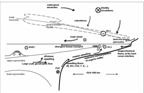
On both eastern and western margins of tropical and subtropical basins, interactions between topographic features, coastal atmospheric jets, coastally trapped and internal waves, Ekman transport and submesoscale and mesoscale circulations (Figure 4) further complicate our ability to represent coastal dynamics in climate models (Richter, 2015). These model biases affect seasonal prediction and climate change projections through non-linear processes such as atmospheric deep convection (Belmadami et al., 2014), and cannot be easily corrected
a posteriori.
Primary production and the fate of organic matter influence the capacity of the coastal oceans to capture atmospheric CO2 (Fiechter et al., 2014). Currently, the net effect of coastal productivity and CO2 flux on the global carbon cycle is highly uncertain. Closely coupled to CO2 atmosphere-ocean exchange is growing concern for acidification and deoxygenation of coastal waters (Ito et al., 2017). While empirical relationships between climate conditions and marine ecosystems have been documented, their stationarity over long time periods is uncertain, particularly as coastal systems are forced by physical climate conditions never observed in the recent observational record (Rykaczewski and Dunne, 2010).
The upwelling that occurs in eastern tropical-subtropical boundary currents is highly sensitive, depending on latitude, to the adjacent surface and subsurface water masses and/or to the coastal wind stress, the so-called coastal low-level jet (LLJ) (Fennel et al., 2012). This sensitivity is reflected in the biogeochemical consequences of the upwelling. The representation of both water masses and coastal wind stress are challenging in numerical models, and observations are lacking and/or are collected at national level with limited international coordination. LLJs are located at the atmospheric low-level inversion capping the planetary boundary layer (PBL) and separate moist, cool marine air-masses from warm, dry continental air-masses. They separate prevalent mid-tropospheric westerlies and lower-mid-tropospheric easterlies, and are due to atmospheric subsidence associated with subtropical anticyclones (Takahashi and Battisti, 2007; Toniazzo et al., 2011). Currently almost no in situ data is available on some of the LLJs, such as that of the Benguela (Patricola and Chang, 2016) and scatterometer satellite data have limitations within the coastal fringe (Astudillo et al., 2017). Even where regular measurements exist (e.g., Chile-Peru and California coasts) stations are land-based and lateral gradient information is sparse.
Western BCs of the subtropical gyres, such as the Gulf Stream, the Kuroshio, the Brazil, the Agulhas, and the East Australian Currents play important roles in climate system. They export heat, salt, and nutrients from the tropics, release vast heat and moisture to the atmosphere, and play important roles in a number of atmospheric phenomena such as precipitation (Minobe et al., 2008), positioning of the storm
track (Small et al., 2014), and blocking and positioning of the jet stream (O’Reilly et al., 2017). Alike eastern boundary upwellings, western boundary currents mediate the horizontal and vertical flux of water masses from the permanent thermocline to the mixed layer (Blanke et al., 2002). They can also have a strong influence on the uptake of carbon dioxide (CO2) from the atmosphere (Takahashi et al., 2009), and thus be a key component of the carbon cycle. The ocean dynamics in the western boundary regions can control the local expression of large-scale sea-level rise on the eastern coasts of the continents (Minobe et al., 2017).
Observing Requirements
Major challenges in observing the BCs and the continental margins include elevated mesoscale and submesoscale variability, the heterogeneity across regions, and the complexity of processes affecting the dynamics and thermodynamics of the air-sea interface. Decades of consistent in situ observations are required to distinguish long-term anthropogenic change from changes associated with natural variability (Takahashi and Martinez, 2017). They are also necessary for better understanding extreme events, including marine heatwaves that often occur in the eastern boundary upwelling systems due to shallow thermocline associated with large-scale climate drivers and/or local air-sea interaction (Bond et al., 2015;
Kataoka et al., 2018).
Multidecadal and interdisciplinary observations are available in some eastern BCs, such as the California (Goericke and Ohman, 2015) or Peru (Graco et al., 2017) Current systems and in all the western boundary currents. However, only baseline observations are available in most coastal oceans, particularly in the southern hemisphere. Given the coastal oceans’ disproportionately large importance to human society and marine ecosystems, continued emphasis should be placed on increasing in-situ observations and sharing existing data collected within national programs.
Boundary current systems observing systems should be developed and implemented to cover the upper 1500 m continental slope in dynamical regions key to ocean-atmosphere interactions that are heavily undersampled (seeTodd et al., 2019
for more insights). Enhanced the monitoring of both eastern and western boundary currents is required to more accurately characterize their variability and change, and campaign-type observational experiments are necessary to improve understanding of the mechanistic processes controlling them.
FIGURE 4 |Schematic of processes at play in Eastern boundary upwelling system (direction of flow corresponds to the northern hemisphere). Arrows represent mass or quantity fluxes. SMM: submesoscale mixing. SGEC, subtropical gyre equatorial current; EBC, Eastern boundary current; PUC, poleward undercurrent; ACJ, atmospheric coastal jet; OCJ, oceanic coastal jet; Gray lines, isopycnals and clouds (dashed). Modified from the one generated at the first EBUS meeting in Ankara in 2016.
due to their sensitive nature in terms of economic (e.g., oil exploration and fish stocks), military and border enforcement considerations. Restrictions also involve sovereign airspace, limiting in situ observations of the atmospheric boundary layer, and which is a critical component of the coupled coastal upwelling system. Height-resolved atmospheric observations are particularly scarce and a major limitation for the understanding of coastal dynamics of upwelling regions.
We argue for fostering finer and more integrated physical and biogeochemical in situ sampling that would naturally involve R/V surveys, autonomous sensors (drifters, profilers, and gliders), and moorings. Considering the general gap in coastal marine in situ data, a specific effort could target the ability of such communities to install and maintain long-term high-frequency ocean-atmosphere data-buoys at homogenous standards, especially in the tropics-subtropics. The ship time and sea-going capacity of various national laboratories for fishery assessment should also be better leveraged. Coordinated coastal process studies in different regions are required to document the relationship between coastal upwelling and meteorological conditions, and to improve understanding of the mechanical and thermal forcing of the near-surface ocean in coastal areas, of surface turbulent fluxes, air-sea exchanges, transport and mixing
at scale of kilometers or less, and biogeochemical exchanges, interactions, and cycling.
OCEAN OBSERVATIONS FOR CLIMATE
MODELING AND CLIMATE
INFORMATION
Background
volcanic eruptions, and internal variability, can be excluded. There is also growing interest about ocean extremes and abrupt events, requiring the observational record to include time-scales of these extremes.
Since OceanObs’09, the role of ocean modeling and data assimilation in furthering understanding and enhancing prediction capabilities has increased to the point where today models and state estimations are integral to oceanography and climate science. In particular, models initialized from observed climate conditions through state estimation products are used in prediction or projection systems. State estimation involves a simultaneous analysis of the state of both ocean and atmosphere. These coupled state estimations will benefit from accurate and complete estimates of the exchange of heat and momentum at the ocean-atmosphere interface, noting the requirement for global balances.
Recent advances in the fidelity of models and their enhanced use arose through ongoing community efforts to improve the numerical and physical foundations of ocean models. These advances also concern the increased role of open source development: by embracing the input of any and all scientists and engineers, and offering a systematic and documented software framework to ingest that input, ocean model codes have been taken from the purview of a few experts circa 2009 into the light of an open and vigorous community circa 2019. Further details of the enhancements to numerics and physics are summarized in Fox-Kemper et al. (2019); here we focus on the role of observations for improving the skill of ocean models as part of assimilation/prediction systems.
From numerical schemes to parameterizations, ocean circulation models have improved over the last decade [see
Griffies et al. (2010) for an assessment a decade ago]. New numerical approaches, including Arbitrary Lagrangian-Eulerian approaches to vertical coordinates and unstructured and nested horizontal grids, preserve large-scale budgets while allowing for regional specificity, and improved stability and accuracy. Coupled models – sea ice, atmosphere, and ocean-ice shelf – are evolving rapidly and reveal emergent phenomena that uncoupled models fail to capture. Consistent coupling requires numerical and parameterization advances that will lead to more robust estimates of oceanic and cryospheric changes, including sea level rise. Significant model biases have been reduced through improved parameterizations of mesoscales, submesoscales, boundary layers (Villas Boas et al., 2019), internal mixing, and other processes, in turn made possible by process-level understanding through high-resolution models and dedicated observational studies.
Requirements for Climate Modeling and
Forecasting
As the community moves into higher-resolution and more accurate modeling, new observational challenges arise ( Fox-Kemper et al., 2019). Continuous monitoring of global and process-level diagnostics is key to ensuring continued progress in model development. At the same time, coordinated sets of observing system simulation experiments (OSSEs) can help
optimizing cost and scale effectiveness of future long-term observational systems (Mazloff et al., 2017).
Key diagnostics and their observational requirements include the annual cycle at various latitudes. In the polar oceans, for example, challenges in observing it within the seasonal ice zone and a bias toward summer values in the observations cause large model uncertainties in surface momentum and buoyancy flux that are, in turn, among the largest sources of model spread (Downes et al., 2015;Farneti et al., 2015). Sea ice thickness, sea ice volume, AABW and High Salinity Shelf Water formation rates and processes, ice shelf basal melt (including rates of changes), iceberg calving rates, and ocean heat fluxes are also among the data-driven products required to meet WCRP research and modeling needs, and reduce divergence in ocean reanalyses (Uotila et al., 2018).
In addition, many new applications of ocean and climate models, especially state estimation, monitoring, and decadal predictions, require observational data that is high quality in representativeness, accuracy, precision, and sampling. Realistic models benefit from these observations, and at the same time provide help to identify gaps in observational schemes.
Observational Products for Climate
Information
Ocean reanalyses (or syntheses) are a fundamental tool for present-day climate monitoring because they provide a dynamically consistent, four-dimensional view of the oceans. Although the propagation of the observational content into unobserved regions or periods is non-trivial, the use of ocean reanalyses products increased significantly during the last decade (Stammer et al., 2016). Ocean reanalyses that combine an ocean general circulation model with available ocean observations use new, improved methods for comparing observations and modeled data. Reanalyses, if consistent mathematically and dynamically, can provide information for key climate diagnostics that are mostly unobserved, such as deep ocean heat content changes and their contributions to sea level rise (Karspeck et al., 2017; Palmer et al., 2017). Synthesis efforts are widely used in climate studies such as the annual State of the Climate report (Blunden et al., 2018), and applications ranging from downstream (biogeochemistry, fishery, and energy) modeling to downscaling (high-resolution regional simulations) deployments, depend upon their availability.
The development and production of ocean reanalyses calls for coordinated efforts in disseminating quality-controlled observational datasets, which may in turn benefit from delayed time quality checks e.g., relying on feedback information from assimilation systems and/or sophisticated buddy checks (e.g.,
Cabanes et al., 2013). Among these datasets, IQuOD is a recently produced collection of marine sub-surface observations, which aims at processing and disseminating unbiased climate data of the highest quality, consistency, and completeness (Domingues and Palmer, 20157). Among many existing datasets, in situ
observations of biogeochemical parameters have been compiled and quality controlled by the global ocean data analysis project
(GLODAP), that includes over one million seawater samples (Olsen et al., 20168). Similar initiatives have been implemented by
several space agencies for satellite parameters (e.g., the European Space agency climate change initiative (CCI), or the Making Earth System Data Records for Use in Research Environments (MEaSUREs) programs through the NASA Earth Science Data Systems). Finally, there is the need to sustain and maintain a large number of observational datasets (e.g., currents from drifters or ADCP, tide-gauge data, air-sea flux measurements, etc.) that are used for validation purposes and enable improvements of, and linkages among, ocean models, and assimilation systems (Balmaseda et al., 2015).
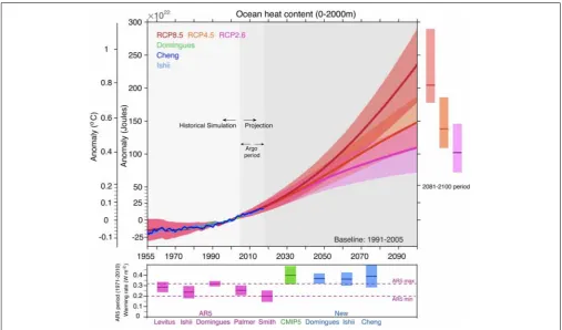
Investigating ocean heat content products, Abrams et al. (2013) concluded that a major source of error was in the interpolation-methods of the underlying time series.Cheng et al. (2017)identified the culprit in assuming in the interpolation that missing data can be treated as background climatological field. This assumption creates a low bias in the estimates, that for global heat content becomes a significant fraction of the trend (Figure 5). New estimates agree better with, and lie with the spread of, CMIP5 simulations of the historical period.
Controlling these biases demands high quality reference temperature dates sets with expendable measurements from Argo and XBT lines from ship of opportunities as done in
8www.glodap.info
the IQuOD project. Additionally, the analysis and gridding of the observations should be monitored through systematic reviews and assessments. Finally, it is essential that the observed records are tested against those from climate models (Figure 5, lower panel).
Critical for reanalyses and objective analyses is the provision of uncertainties for each observational based product, ideally in form of error covariances. However, uncertainty information needs to be provided also for model results, and in either case should account for omissions, sampling and systematic errors.
Finally, an important downstream application is the initialization of coupled subseasonal to decadal prediction systems (Marotzke et al., 2016), where improved data assimilation schemes have led to increased predictability (Bellucci et al., 2011;
Polkova et al., 2014;Liu et al., 2017). However, model-consistent coupled assimilation schemes will ultimately be required to optimize prediction skills and improve model biases.
SUMMARY AND FINAL REMARKS
[image:13.595.44.552.371.669.2]Climate monitoring requires long, sustained and high-quality measurements of essential and process-oriented climate parameters in the ocean, including surface fluxes of heat, freshwater, and momentum. For climate purposes, the
length of uninterrupted timeseries, and the stability of the measurements are critical.
The climate observing system needs to include both satellite
andin situobservations. A mix of platforms and technologies,
in orbit and in situ, will greatly improve the chance to meet user requirements, regionally, and globally. Synergies between all components and platforms are fundamental also to insure the cross-calibration of parameters for quality purposes. Each satellite mission should have an in-situ counterpart that optimizes data calibration, stability and space/time sampling, and vice versa. Such a system is parameter oriented; to maximize its use and utility, the subsequent required step is the merging of observations into a parameter time series. Ocean and climate syntheses are therefore an integral part of this endeavor.
Subsurface measurements are critical to monitor and investigate the ocean role in the climate system. It is a priority to expand the Argo program to the full water column and under sea ice, and to augment high-quality sections and timeseries networks, especially in BCs. A global, continuous,in situnetwork of gliders would contribute effectively toward this objective. All existing elements should include O2 and CO2 sensors, as well as nutrient monitoring, a testimony of the increasingly interdisciplinary nature of climate science. Improving both quality and coverage of surface flux measurements of heat, carbon, freshwater, and momentum is mandatory. At the same time the existing satellite fleet should be sustained and expanded, to ensure that surface salinity, gravity, and winds etc are part of a long-term, stable monitoring system.
The climate observing system cannot be static, but needs to evolve scientifically and technically, considering new sampling needs, new sensors and technological advances. Reviewing the adequacy of present-day observing system and its future requirements will allow to focus research and innovation in areas where existing technologies do not meet expectations and needs. Finally, building and sustaining a climate observing system in the ocean relies critically on capacity building, cooperation, and coordination among the international community. It is indispensable to motivate and support the scientific communities
in emerging and developing economies to take ownership for long-term, quality-controlled climate observations, and to use them to produce actionable climate information. This last step is indispensable to the generation of regionally relevant climate information.
AUTHOR CONTRIBUTIONS
DS and AB created the outline of topics and wrote the proposal of the manuscript. All authors contributed to the writing and editing processes of the manuscript, and recommended the references and examples.
FUNDING
This work was partly supported by the DFG funded excellence center CliSAP of the Universituat Hamburg (DS). AB was supported by the National Science Foundation through award NSF-1658174 and by the NOAA through award NA16OAR4310173. SM was supported by the Earth Systems and Climate Change Hub of the Australian Government’s National Environmental Science Program.
ACKNOWLEDGMENTS
Comments from the two reviewers are gratefully acknowledged. We thank all the CLIVAR panel members who contributed with helpful comments and suggestions to this work. The International Cooperation that CLIVAR enjoys would not be possible without the organizational leadership of the CLIVAR ICPO hosted by the First Oceanographic Institute (FIO) in Qingdao, China, the continuous support of the US-CLIVAR office, and the scientific leadership and support of the World Climate Research Programme. NCAR is sponsored by the US National Science Foundation. BD acknowledges supports from FONDECYT (project 1171861).
REFERENCES
Abernathey, R. P., Cerovecki, I., Holland, P. R., Newsom, E., Mazloff, M., and Talley, L. D. (2016). Water-mass transformation by sea ice in the upper branch of the Southern Ocean overturning.Nat. Geosci.9, 596–601. doi: 10.1038/ ngeo2749
Abrams, J. P., Baringer, M., Bindoff, N. L., Boyer, T., Cheng, L. J., Church, J. A., et al. (2013). A review of global ocean temperature observations: implications for ocean heat content estimates and climate change.Rev. Geophys.51, 450–483. doi: 10.1002/rog.20022
Astudillo, O., Dewitte, B., Mallet, M., Frappart, F., Ruttlant, J., Ramos, M., et al. (2017). Surface winds off Peru-Chile: observing closer to the coast from radar altimetry.J.Rem. Sens. Environ.191, 179–196. doi: 10.1016/j.rse.2017.01.010 Balmaseda, M. A., Hernandez, F., Storto, A., Palmer, M. D., Alves, O., Shi, L.,
et al. (2015). The ocean reanalyses intercomparison project (ORA-IP).J. Operat.
Oceanogr.8, s80–s97. doi: 10.1080/1755876X.2015.1022329
Bellucci, A., Gualdi, S., Masina, S., Storto, A., Scoccimarro, E., Cagnazzo, C., et al. (2011). Decadal climate predictions with a coupled OAGCM initialized with oceanic reanalyses.Clim. Dyn.40, 1483–1497. doi: 10.1007/s00382-012-1468-z
Belmadami, A., Echevin, V., Codron, F., Takahashi, K., and Junquas, C. (2014). What dynamics drive future wind scenarios for coastal upwelling off Peru and Chile? Clim. Dyn. 43, 1893–1914. doi: 10.1007/s00382-013-2015-2
Blanke, B., Speich, S., Madec, G., and Maugé, R. (2002). A global diagnostic of interior ocean ventilation.Geophys. Res. Lett.29, 108-1–108-4.
Blunden, J., Arndt, D. S., and Hartfield, G. (eds). (2018). State of the climate in 2017.Bull. Am. Meteorol. Soc.99:Si-S310. doi: 10.1175/2018BAMSStateofthe Climate.1
Bond, N. A., Cronin, M. F., Freeland, H., and Mantua, N. (2015). Causes and impacts of the 2014 warm anomaly in the NE Pacific.Geoph. Res. Lett.42, 3414–3420. doi: 10.1002/2015GL06330
Bourassa, M. A., Gille, S. T., Bitz, C., Carlson, D., Cerovecki, I., Clayson, C. A., et al. (2013). High latitude ocean and sea ice surface fluxes: challenges for climate research.Bull. Am. Meteorol. Soc.94, 403–423. doi: 10.1175/BAMS-D-11-00244.1
Breitburg, D., Levin, L. A., Oschlies, A., Grégoire, M., Chavez, F. P., Conley, D. J., et al. (2018). Declining oxygen in the global ocean and coastal waters.Science