using a wavelet multiresolution analysis
.
White Rose Research Online URL for this paper:
http://eprints.whiterose.ac.uk/74606/
Monograph:
Guo, L.Z., Billings, S.A. and Coca, D. (2007) Multiscale identification of spatio-temporal
dynamical systems using a wavelet multiresolution analysis. Research Report. ACSE
Research Report no. 947 . Automatic Control and Systems Engineering, University of
Sheffield
[email protected] https://eprints.whiterose.ac.uk/
Reuse
Unless indicated otherwise, fulltext items are protected by copyright with all rights reserved. The copyright exception in section 29 of the Copyright, Designs and Patents Act 1988 allows the making of a single copy solely for the purpose of non-commercial research or private study within the limits of fair dealing. The publisher or other rights-holder may allow further reproduction and re-use of this version - refer to the White Rose Research Online record for this item. Where records identify the publisher as the copyright holder, users can verify any specific terms of use on the publisher’s website.
Takedown
If you consider content in White Rose Research Online to be in breach of UK law, please notify us by
Multiscale identification of spatio-temporal dynamical systems
using a wavelet multiresolution analysis
Guo, L. Z., Billings, S. A., and Coca, D.
Department of Automatic Control and Systems Engineering
University of Sheffield
Sheffield, S1 3JD
UK
Multiscale identification of spatio-temporal
dynamical systems using a wavelet multiresolution
analysis
Lingzhong Guo,
Stephen A Billings,
and Daniel Coca
Abstract— In this paper, a new algorithm for the multiscale
identification of spatio-temporal dynamical systems is derived. It is shown that the input and output observations can be represented in a multiscale manner based on a wavelet multires-olution analysis. The system dynamics at some specific scale of interest can then be identified using an orthogonal forward least-squares algorithm. This model can then be converted between different scales to produce predictions of the system outputs at different scales. The method can be applied to both multiscale and conventional spatio-temporal dynamical systems. For multiscale systems, the method can generate a parsimonious and effective model at a coarser scale while considering the effects from finer scales. Additionally, the proposed method can be used to improve the performance of the identification when measurements are noisy. Numerical examples are provided to demonstrate the application of the proposed new approach.
Index Terms— Multiscale identification, spatio-temporal
sys-tem, orthogonal least squares algorithm, multiresolution analysis
I. INTRODUCTION
T
HE identification of spatio-temporal systems has recievedincreasing attention in recent years with applications in a variety of scientific and engineering areas (Voss, Bunner, Abel 1998, Coca and Billings 2001, 2002, McSharrya, Elle-polab, von Hardenberga, Smitha, Kenning 2002, Yan, Hu, Zhou, and Liu 2004, Billings, Guo, and Wei 2006, Guo and Billings 2006, Guo, Billings, and Wei 2006). Both discrete and continuous time models have been developed including coupled map lattice (CML) models, lattice dynamical system (LDS) models, and partial differential equations (PDE) to describe the underlying spatio-temporal dynamical systems based on observations of the system response. In addition, many useful identification algorithms have also been derived for the detection of the system structure, determination of the unknown system parameters, and the removal or modelling of noise. However, identifying a model of a spatio-temporal system from observations is still far from straightforward. Among the major difficulties that remain, two will be given special attention in this paper. The first arises from multiscale problems, and the second is associated with noise on the observations.
Multiscale phenomena have been widely observed in many diverse fields including physics, chemistry, biology, ecol-ogy, and network traffic systems (Mandelbrot 1967, Car
The authors are with the Department of Automatic Control and Systems Engineering, The University of Sheffield, Sheffield, S1 3JD, UK.
and Parrinello 1985, Littlewood and Maniatty 2005, Lorenz 1996, Chaudhari, Yan, and Lee 2003, Bindal, Khinast, and Ierapetritou 2003, Muller-Buschbaum, Bauer, Pfister, Roth, Burghammer, Riekel, David, and Thiele 2006, Louie and Kolaczyk 2006, Huerta, Rabinovich, Abarbanel, Bazhenov 1997, Feldmann, Gilbert, Willinger, and Kurtz 1998, Eck 2004). There are also a variety of multiscale systems including chaotic systems, molecular dynamics, and solar systems. Due to the presence of different scales, modelling, analysis and prediction of multiscale problems often involves the problem of how to describe the interactions between the different laws of physics at different scales, how to analyse the properties of such systems both qualitatively and quantitatively, how to cope with irregularly sampled data, and how to obtain exact/approximate solutions either analytically or numerically. All these problems require new methods and tools to find a solution. Existing methods of modelling, analysis and computation of multiscale systems include Fourier analysis, multigrid methods, domain decomposition methods, fast mul-tipole methods, adaptive mesh refinement methods, wavelet-based methods, homogenisation methods, quasi-continuum methods, and the Heterogeneous Multiscale Method (HMM) (see reviews given by E and Engqiust (2003), E, Engquist, Li, Ren, and Vanden-Eijnden (2006) and references therein). Considering the difficulties of modelling such systems, it would be advantageous if a model could be identified from the observed multiscale data. The model could then be used for the analysis of system behaviour or in control. To the best of our knowledge, there is currently very little research on the identification problem for multiscale systems from observed data and this important problem will therefore be studied in this paper.
In this paper, a new solution to the identification problem of spatio-temporal dynamical systems directly from observations is proposed to tackle the above mentioned two difficulties. The idea behind the proposed method is that an infinite dimensional spatio-temporal system is projected onto a finite dimensional subspace using a wavelet multiresolution analysis so that the system can be viewed at different scales. It has been shown in Coca and Billings (2002) that the wavelet coefficients at a scale form a finite dimensional system of ordinary differential equations which can be used to represent an finite dimensional approximation at some scale of the original system . The system dynamics at a specific scale of interest can then be identified using an orthogonal forward regression (OFR) least-squares algorithm (Billings, Chen, and Kronenberg 1989). It is shown that this model can then be converted between different scales to produce predictions of the system outputs at dif-ferent scales using wavelet decomposition and reconstruction techniques. Because of the filtering properties of wavelets it is also shown that the new method naturally combines the identification procedure with a filtering process.
Section 2 presents a multiscale representation of spatio-temporal dynamical systems using a wavelet multiresolution analysis. In section 3, the identification method and the imple-mentation strategy are presented including a discussion about the properties of the OFR algorithm. Section 4 illustrates the proposed approach using some examples. Finally conclusions are drawn in section 5.
II. AMULTISCALE REPRESENTATION OF
SPATIO-TEMPORAL DYNAMICAL SYSTEMS
Consider the following evolution equation of a spatio-temporal dynamical system
du
dt +Lu=f, u(0) =u0 (1)
where L : V → V∗ is a nonlinear operator with V ⊂
L2(Ω) a Sobolev space, and where Ω ⊂ Rn is a nice
spatial domain. The evolution of equation (1) can represent a partial differential equation model for both conventional and multiscale spatio-temporal dynamical systems.
To generate a multiscale representation of the system (1),
let Vj ⊂V, j ∈Z be a multiresolution approximation of the
spaceV. That is,Vj, j∈Zis an increasing sequence of closed
subspaces ofL2(Ω)with the following properties (Chui, 1992)
1) Vj ⊂Vj+1,
2) f(x)∈Vj⇐⇒f(2x)∈Vj+1, j∈Z,
3) S
j∈ZVj is dense in L2(Rn)and
T
j∈ZVj =∅,
4) A scaling function φ(x) ∈ V0 exists such that the set
{φ(x−k)|k∈Zn} forms a Riesz basis ofV
0.
Following the definition of the multiresolution analysis, the set
of functions{φj,k = 2j/2φ(2jx−k)} is a Riesz basis ofVj.
Let Wj be a complementary space of Vj inVj+1, such that
Vj+1 =VjLWj. Consequently
M
j∈Z
Wj =L2(Rn). (2)
Wj is called a wavelet subspace. A functionψ(x)is a wavelet
if the set of functions {ψ(x−k)|k ∈ Zn} is a Riesz basis
of W0. It follows that the set of wavelet functions {ψj,k =
2j/2ψ(2jx−k)} is a Riesz basis of L2(Rn).
At resolution j the projection Pj (resp. Qj) of a function
f onto Vj (resp. Wj) that corresponds to the above split of
L2(Rn)can be written with the use of a dual scaling function
˜
φ(resp. dual wavelet functionψ˜) as follows
Pjf(x) =
X
k
< f,φ˜j,k> φj,k(x) (3)
Qjf(x) =
X
k
< f,ψ˜j,k> ψj,k(x)
where < · > denotes the inner product. Such wavelets are
called biorthogonal wavelets. Generally, φ˜ 6= φ and ψ˜ 6= ψ
except when orthogonality holds. The definition of a
multires-olution analysis implies that for anyf(x)∈L2(Ω)
lim
j→∞Pjf(x) =f(x)
(4)
f(x) =X
j
Qjf(x).
Since Wj is the complementary subspace of Vj in Vj+1,
that is Vj+1 = VjLWj, it follows that Pj+1f(x) =
Pjf(x) +Qjf(x). This gives an alternative representation of
the projection of a function f ∈ L2(Ω) at resolution j+ 1
using both the scaling and wavelet functions as
Pj+1f(x) = X
k
< f,φ˜j,k> φj,k(x)+
X
k
< f,ψ˜j,k> ψj,k(x).
(5)
In this way, it is understood that the projection Pj provides
an approximation of the functionf at some resolutionj and
the details left by this approximation are contained inQj. By
iteration, a wavelet decomposition can be obtained as follows
Pj+1f(x) = X
k
< f,φ˜j−l,k> φj−l,k(x) (6)
+
j
X
i=j−l
X
k
< f,ψ˜i,k > ψi,k(x).
It should be noted that a discretisation of (1) can be
considered as replacing (1) with an approximation in Vj+1.
The operatorLis replaced by a operatorLj+1:Vj+1→Vj+1
defined by
< Luj+1, wj+1>=< Lj+1uj+1, wj+1>, wj+1 ∈Vj+1.
(7) Then the discretised dynamics of the system (1) at a
scale/resolutionj+ 1can be described as the following initial
value problem inVj
duj+1
where uj+1(t, x) = Pj+1u(t, x) = Pk <
u(t, x),φ˜j+1,k(x) > φj+1,k(x) and fj+1(t, x) = Pj+1f(t, x) =Pk < f(t, x),φ˜j+1,k(x)> φj+1,k(x).
Consider the decompositionVj+1=Vj⊕Wj, the projection
from Vj+1 ontoVj andWj yields
uj(t, x) = Pjuj+1(t, x) = X
k
uj,k(t)φj,k(x) (9)
fj(t, x) = Pjfj+1(t, x) = X
k
fj,k(t)φj,k(x)
on Vj withuj,k(t) =< uj+1(t, x),φ˜j,k(x)>andfj,k(t) =<
fj+1(t, x),φ˜j,k(x)>, and
u′
j(t, x) = Qjuj+1(t, x) =
X
k
u′
j,k(t)ψj,k(x) (10)
f′
j(t, x) = Qjfj+1(t, x) =
X
k
f′
j,k(t)ψj,k(x)
onWj withu′j,k(t) =< uj+1(t, x),ψ˜j,k(x)>andfj,k′ (t) =<
fj+1(t, x),ψ˜j,k(x)>, which satisfies
uj+1(t, x) = uj(t, x) +u′j(t, x) (11)
fj+1(t, x) = fj(t, x) +fj′(t, x).
Applying the projectionsPj andQj to eqn. (8) generates the
following two equations
duj
dt +PjLj+1(uj+u
′
j) = fj (12)
du′
j
dt +QjLj+1(uj+u
′
j) = f
′
j.
Following the Corollary 3.1 (Coca and Billings 2002), there exists a finite dimensional system of ordinary differential
equations with the wavelet coefficients {uj,k, u′j,k}j and
{fj,k, fj,k′ }j as the output and input of the system such
that uj(t, x) =Pkuj,k(t)φj,k(x) forms a finite dimensional
approximation at the scale j of the solution of the original
system. Furthermore, this finite dimensional system of ordi-nary differential equations can generally be decoupled into two effective equations: one describes the coarse dynamics at
scale j
duj,k
dt =Fj(uj,k(t), fj,k(t), f
′
j,k(t)) (13)
and the second describes the corresponding detailed dynamics for this scale
du′
j,k
dt =F
′
j(u
′
j,k(t), fj,k(t), fj,k′ (t)). (14)
By repeating the above decomposition process, a multiscale representation as eqns. (13) and (14) of the original spatio-temporal dynamical system is obtained.
It should be noted that eqn. (13) represents an
approxima-tion to the original dynamical systems at scalej. The presence
of the detailsf′
k,j in eqn. (13) indicates that the influence from
a finer scale is accommodated within this model.
III. MULTISCALE IDENTIFICATION OF SPATIO-TEMPORAL
DYNAMICAL SYSTEMS
For spatio-temporal dynamical systems, experimental mea-surements are often available in the form of a series of
snapshotsu(x, n∆t),n= 0,1,2,· · ·,x∈Ω, where∆tis the
time sampling interval. Assume the system to be considered
is spatially sampled at a sampling interval ∆x, then the
observations are discrete measurementsu(xi, tj)both in time
and space. This is equivalent to replacing the original system
in the infinite dimensional space V with an approximation
in some finite dimensional subspaceVj. The objective of the
identification is to obtain one model for the system from these observations.
A. Comments on multiscale identification problems
As mentioned earlier, the objective of multiscale identi-fication for spatio-temporal dynamical systems is to obtain an effective model or a set of models from observed spatio-temporal patterns. Eqns. (13) and (14) at any scale can be used to describe the underlying spatio-temporal dynamics at that specific scale once the representation is estimated or extracted by using some identification algorithm. Ideally, the identification technique should be able to produce a concise model structure with a low spatial dimension. This ensures that the obtained model is parsimonious and can readily be interpreted either for simulation or analysis. Once eqns. (13) and (14) are approximated by some function space such as polynomials, they will be in the form of a linear-in-the-parameters model, therefore, theoretically any least-squares-type algorithm can be employed to produce a model. However, there are several problems related to multiscale identification which also need to be addressed:
1) Choosing the proper approximation subspaceVj, that is
the mesh size over a spatial domain is very important. In identification, the mesh size represents the sampling period in the spatial domain and reflects the number of measurement locations and determines the scale of interest. In the case that the mesh size can be made sufficiently small, a system model can theoretically be identified using the data from the finest scale, which can resolve the dynamical behaviours at all scales. However, the finer the mesh size is, the higher the dimension of the approximation subspace becomes, that means the dimension of the resulting finite dimensional model will be extremely large and computationally expensive if not formidable. In this case, it is worth considering projecting the data into a coarser scale to obtain a lower dimensional and effective model. In some other cases, it will be of interest to construct system equations on a coarse scale that account for the contributions from these finer scales, such as in molecular dynamics. These requirements translate into the need to identify an effective and economical model for the coarse scale with a lower dimension.
scales directly from the measurements. However, the observations from the best obtainable scale can be used to identify a model at the specific scale, which represents a coarse behaviour of the original system and it would be beneficial if an equivalent finer model could be obtained whose solutions have the same coarser behaviour as the original unknown complicated systems.
3) The presence of noise on the measured data can affect the accuracy of the identified models.
To overcome these problems, in this paper a new approach is proposed by applying the Orthogonal Forward Regression (OFR) least-squares algorithm to data at some available scale. The proposed method has the following characteristics.
1) The proposed method does not assume any a priori knowledge regarding the structure or parameters of the underlying spatio-temporal dynamical system.
2) The measured data are not limited to the finest scale. In the case that the system can be observed at the finest scale, the proposed method can be used to obtain a simpler model at some coarse scale and this identified model can be used to predict the outputs of the system at different scales including the finest scale. In the case that the system can not be measured at its finest scale, a coarser model can be identified at some observable scale, by which an approximation of the finest scale behaviour can be made.
3) The multiscale representation using wavelets provides a natural filter for systems with measurement noise. This is because the coarser the data are, the less the noise is. 4) The OFR least-squares algorithm can effectively deter-mine the model structure and provide parameter esti-mates in a forward term selection manner.
In what follows, the multiscale identification method and some simulation examples will be presented.
The multiscale identification algorithm proposed in this paper can be summarised as follows.
1) Perform a multiresolution analysis for the measured data to obtain a multiscale representation of the system. 2) Choose a suitable scale and apply the OFR algorithm to
generate a model structure and parameter estimates. 3) Using wavelet decomposition and reconstruction
meth-ods predict the outputs of the system at different scales.
B. The OFR algorithm
Given a set of (candidate terms) basis functions from a regressor class, the objective of the identification algorithm is to select the significant terms from this set while estimating the corresponding monomial coefficients. In this paper, the OFR least-squares algorithm is applied to a set of polynomial basis functions. The OFR algorithm involves a stepwise or-thogonalisation of the regressors and a forward selection of the relevant terms based on the Error Reduction Ratio criterion. The algorithm provides the optimal least-squares estimate of the polynomial coefficients.
Formally, the classical OFR least-squares algorithm can be stated as follows (Billings, Korenberg, and Chen 1988).
Consider the following linear relationship
y(t) =
n
X
i=1
θipi(t) +ξ(t) (15)
wherepi(t)are regressors andy is the dependent variable.
Letp0(t), p1(t),· · ·, pn(t)andy(t),t= 1,2,· · ·, N be the
series of observations. Denote Y = (y(1), y(2),· · ·, y(N))T
and Pi = (pi(1), pi(2),· · ·, pi(N))T, i = 0,1,· · ·, n, then the following linear regression model can be formed
Y =P θ+ Ξ (16)
where P = (P0, P1,· · ·, PN) is the regression matrix,
θ = (θ1, θ2,· · ·, θn)T represents the unknown parameters
to be estimated, and Ξ = (ξ(1), ξ(2),· · · , ξ(N))T is some
modelling error vector.
Assume that the matrix PTP is symmetric and positive
definite, the matrix decomposition theorem states that the
matrixPTP can be repressed as
PTP =ATDA (17)
whereA is a unit upper-triangle matrix withA−1A=I and
D is diagonal with all positive elements. Then (16) can be
written as follows
Y =P θ+ Ξ =P(A−1A)θ+ Ξ =XAθ+ Ξ =Xg+ Ξ (18)
whereX=P A−1 is anN×(n+ 1)matrix with orthogonal
columns Xi such that XTX = D, and g = Aθ. The
orthogonal least squares solutionˆg to (18) is then given by
ˆ
g=D−1XTY. (19)
The parametersgˆandθˆsatisfy the triangular equation
Aθˆ= ˆg. (20)
Because of the orthogonality properties, the termXi and the
quantitygi can be calculated in an independent manner. This
is achieved by applying the algorithm in a forward way with the error reduction ratio (ERR) as selection criterion at each
step. The ERR caused by termi,i= 0,1,· · ·, nis defined as
ERRi=
g2
iXiTXi
YTY . (21)
C. Properties of the OFR least-squares algorithm
In order to discuss the properties of the OFR algorithm, some assumptions are needed.
Assumption 1: There is no undermodelling, that is, the
input-output data was generated by some true dynamic system
that can be represented by (15) with the parameters θi, i =
1,· · · , n, and the system is input-output bounded uniformly with probability one.
Assumption 2: ξ(t) is a zero mean white sequence with
a finite covariance σ2 and is uncorrelated with p
i(t), i =
Assumption 3: All processes involved are (jointly) ergodic
of at least second order and the inputs are persistently exciting of sufficiently high order with probability one.
Assumption 4: The matrixPTP is symmetric and positive definite.
From (19)
ˆ
g=D−1XTY =D−1XT(Xg+ Ξ) =g+D−1XTΞ. (22)
Let˜g= ˆg−g, then it is easy to show that under Assumptions
1 and 2 the estimates will be unbiasedE{ˆg}=g(Korenberg,
Billings, Liu, and Mcilroy 1988).
In what follows, the convergence issue of the OFR algorithm
will be addressed. Here, ˆg will be written as ˆg[N] to indicate
that there areN observations used for identification. Note that
the covariance of the parameter error ˜g[N] is given by
cov(˜g[N]) =E{(ˆg[N]−g)(ˆg[N]−g)T}=σ2(XTX)−1. (23)
From (23) and PTP = ATXTXA with A a unit
upper-triangle matrix, the following result can be given
Theorem 1. Under Assumptions 1 and 2,
lim
N→∞k˜g
[N]k= 0 (24)
if and only if
lim
N→∞λ(P
TP) =∞ (25)
or equivalently
lim
N→∞λ(X
TX) =∞ (26)
where k · k denotes the Euclidean norm and λ(M) is the
minimum eigenvalue of the matrixM.
Theorem 2. Under Assumption 1 to 4 limN→∞gˆ[N] =g
with probability one.
Outline of the proof. Assumptions 1 and 3 mean the system is input-output bounded uniformly and there is no
any particular eigenvector of PTP along with the energy
of the system is concentrated with probability one and it follows that the ratio of the largest to the smallest eigenvalues
of PTP is bounded uniformly in N with probability one.
Then according to Aderson and Taylor (1979), it only needs
to prove that limN→∞λ(PTP) = ∞ with probability one.
This is equivalent to showing limN→∞λ(XTX) = ∞ with
probability one. Note that XTX is a diagonal matrix as
XTX =
PN
t=1X02(t)
PN
t=1X12(t)
. ..
PN
t=1Xn2(t)
(27)
Note that PN
t=1Xi2(t), i = 0,1,· · ·, n are the
eigenvalues of PTP. Without loss of generality, let
PN
t=1X02(t) be the minimum eigenvalue of XTX. Suppose
limN→∞
PN
t=1X02(t) <∞ with probability one, then there
must exist an integer T > 0 such that X0(t) = 0 for all
t ≥ T with probability one, which is in contradiction with
Assumption 3.
D. Predictions between different scales
Once a system model at certain scale is identified, it can be used to calculate the wavelet coefficients at different scales in terms of the wavelet decomposition and reconstruction method.
DecompostionVj =Vj−1⊕Wj−1:
ul,j−1(t) = X
k
hk−2luk,j(t) (28)
u′
l,j−1(t) =
X
k
gk−2luk,j(t)
wherehandg are the wavelet filter coefficients.
ReconstructionVj+1=Vj⊕Wj:
ul,j+1(t) = X
k
hl−2kuk,j(t) +
X
k
gl−2ku′k,j(t) (29)
wherehandg are the wavelet filter coefficients.
Note that if the details at all scales are available, then the reconstruction process (29) can be carried out up to the finest scale. If the details are not available, the reconstruction process can still be performed by just ignoring all the details at finer scales. In this case, the obtained prediction is an approximation of the original behaviours at these finer scales.
E. Noise reduction analysis
The presence of noise in the observations generally prevents the OFR algorithm from selecting the correct terms in the model and consequently can produce erroneous parameter
estimates. The relationship between the values of ERRi and
the signal-to-noise ratio has been analysed in detail in Guo and Billings (2007). Here a brief discussion is given.
Note that from the definition of ERR (21), it can be observed that the OFR is equivalent to maximising the product moment correlation coefficient. In fact, the product moment correlation
coefficientρi of termi satisfies
ρ2i =
cov(Y, Wi)2
var(Y)var(Wi) =ERRi
(30)
Letρ¯i be the correlation coefficient of the termi obtained
from noisy data, then
¯
ρi =
ηY
p
η2
Y + 1
s
< Wi, Wi>
<W¯i,W¯i >
ρi (31)
+
i−1
X
j=0
< Pi, Wj >
< Wj, Wj>
ηY
p
η2
Y + 1
s
< Wj, Wj>
<W¯i,W¯i>
ρj
−
i−1
X
j=0
<P¯i,W¯j >
¯
Wj,W¯j
s
<W¯j,W¯j>
<W¯i,W¯i>
¯
where P¯ and W¯ are the noisy version of P and W.
ηY = var(Y)/σε2 with ε the output noise. Note that ηY =
var(Y)/σ2
ε can be considered as the signal-to-noise ratio.
From (31) it can be observed that when the signal-to-noise
ratio is sufficiently high, then ρ¯ will be sufficiently close to
the true value ρ. Therefore it is highly desirable to have a
signal with a high signal-to-noise ratio. Wavelet decomposition provides such a way to reduce the noise from observations and therefore increase the signal-to-noise ratio. By applying a wavelet multiresolution analysis to the data space, a set of coarser signals with high signal-to-noise ratios can be obtained. It follows that an accurate model can be obtained from data at a coarse scale. It can be expected that better predictions of the system behaviour at different scales can be given by using such an accurate model.
IV. SIMULATION STUDIES
A. Example 1 - Non-homogeneous wave equation
Consider the following non-homogeneous wave equation
∂2u(t, x)
∂t2 −C
∂2v(t, x)
∂x2 =f(t, x), x∈[0,1] (32)
with initial conditions
u(0, x) = 0 (33)
du(0, x)
dt = 4exp(−x) +exp(−0.5x)
where
f(t, x) =−13exp(−x)cos(1.5t)−9.32exp(−0.5x)cos(2.1t)
(34)
For C = 1.0 the exact solution u(t, x) of the initial value
problem (32), (34) is
u(t, x) = 4exp(−x)cos(1.5t) + 2exp(−0.5x)cos(2.1t)(35)
−4exp(−x)exp(−t)−2exp(−0.5x)exp(−0.5t)
The measurement function was taken as
y(t, x) =u(t, x) (36)
The reference solution was sampled at 24 = 16 equally
spaced points over the spatial domain Ω = [0,1], x =
{x0,· · ·, x15}. This sampling process can be viewed as
re-placing (35) with an approximation in a finite dimensional
subspace Vn, n = 4. From each location, 1000 input/output
data points sampled at ∆t =π/105were generated. To test
the performance of the proposed approach, a sequence of
noise with zero-mean and variance0.01is added to the output
y(t, x), which results in a signal-to-noise ratio of 26.212dB.
After applying a single level wavelet decomposition with Haar wavelets (other wavelets can be also used), a coarse
approximation of the original data in subspace Vn−1 was
obtained with a signal-to-noise ratio of 29.256dB. Note that
the signal-to-noise ratio has been increased for the signal at the
Terms Estimates ERR STD
yi(t−1)) 1.8166e-001 9.9598e-001 2.1673e-001
yi(t−2)) 1.3340e-001 5.8750e-004 2.0024e-001
yi+1(t−1)) 6.8620e-002 6.1609e-004 1.8140e-001
yi−1(t−1)) 1.3783e-001 4.4141e-004 1.6658e-001
yi−1(t−2)) 2.3862e-001 1.2535e-004 1.6212e-001
u′
i(t−2) 8.4634e+000 1.3364e-005 1.6160e-001
u′
i(t−1)) -8.4172e+000 1.0446e-003 1.1793e-001
ui(t−1) -2.0234e-001 7.3185e-005 1.1429e-001
ui(t−2) 1.9207e-001 9.5179e-005 1.0932e-001
yi+1(t−2) 1.8647e-001 3.4899e-005 1.0744e-001
constant 1.2969e-004 1.2338e-009 1.0744e-001
TABLE I
EXAMPLE1: THE TERMS AND PARAMETERS OF THE FINAL MODEL AT THE
COARSE SPACEVn−1
0 200 400 600
800 1000
0 5 10 15 −10
−5 0 5 10
t x
y(t,x)
Fig. 1. Example 1: Spatio-temporal signal at the original scalen= 4
coarse scale and this should significantly increase the accuracy of the model. The data are plotted in Fig.(1) and Fig.(2).
In this simulation, a model at the coarse scale is to be
identified. The inital neighbourhood was selected to bei−1
and i+ 1 in the spatial domain andt−1, t−2 in the time
domain. A set of 200 observations randomly selected among the data set was used for identification. In addition, 200 input
and output dataui(t), yi−1(t)andyi+1(t)from neighbouring
locationsi−1, i+ 1acted as inputs during the identification.
The identified model using the OFR least squares algorithm with a linear model structure, are listed in Table (I), where ERR denotes the Error Reduction Ratio and STD denotes the standard deviations.
The model predicted output of the identified model is plotted in Fig.(3). Fig.(4) shows the model predicted error between the exact solution and the identified CML model predicted output. Although there are errors between the real output and the model predicted output it is clearly observed that the identified
CML model is able to reproduce the system behaviour inVn−1
with very high fidelity. Furthermore, the obtained model in Table (I) was used to produce a prediction for the system
behaviour at the original scalen= 4. The prediction has been
[image:8.595.329.551.102.228.2]0 200 400 600
800 1000
0 2 4 6 8 −10 −5 0 5 10
t x
y(t,x)
Fig. 2. Example 1: Spatio-temporal signal at single-level coarser scalen−1
0 200 400
600 800 1000
0 2 4 6 8 −10 −5 0 5 10
t x
[image:9.595.356.522.115.233.2]y(t,x)
Fig. 3. Example 1: Model predicted output at the coarse scale
0 200 400
600 800 1000
0 2 4 6 8 −1 −0.5 0 0.5 1
t x
[image:9.595.94.260.118.240.2]e(t,x)
Fig. 4. Example 1: Model predicted error at the coarse scale
0 200 400
600 800 1000
0 5 10 15 −10
−5 0 5 10
t x
y(t,x)
Fig. 5. Example 1: Model predicted output with high frequency detail at the original scale using the identified coarse model
0 200 400 600
800 1000
0 5 10 15 −1 −0.5 0 0.5 1
t x
[image:9.595.357.522.291.410.2]e(t,x)
Fig. 6. Example 1: Model predicted error with high frequency detail at the original scale using the identified coarse model
0
200 400 600
800 1000
0 5 10 15 −10
−5 0 5 10
t x
[image:9.595.94.259.294.410.2]y(t,x)
Fig. 7. Example 1: Model predicted output without high frequency detail at the original scale using the identified coarse model
B. Example 2 - Two-dimensional deterministic CML
Consider the following two-dimensional deterministic CML with symmetrical nearest neighbour coupling
xi,j(t) = (1−ε)f(xi,j(t−1)) +
ε
4(f(xi,j−1(t−1)) (37)
+f(xi,j+1(t−1)) +f(xi−1,j(t−1)) +f(xi+1,j(t−1)))
wherexi,j(t)i, j = 1,· · ·, N is the state of the CML located
at site (i, j) at discrete time t, ε is the coupling strength,
and N is the size of lattice. Periodic boundary conditions,
that is x1,j(t) = xN,j(t), xi,1(t) = xi,N(t) for all i, j and
t, are used throughout this study. The evolution of the CML
on the lattice sites is governed by the local mapf, which is
generally a nonlinear function chosen to be the logistic map in this simulation
f(x) = 1−ax2. (38) This model has been extensively studied. It has been observed
that for small ε (< 0.3) the system evolves from a frozen
random state to pattern selection and to fully developed spatio-temporal chaos via spatio-spatio-temporal intermittency. For stronger
couplingε >0.3neither a frozen random pattern nor a pattern
selection regime is formed which implies there are no pattern changes in this case (Kaneko 1989).
The model (37) with (38) was simulated for a lattice of
the size 50 × 50 with random initial conditions, periodic
[image:9.595.90.259.467.585.2] [image:9.595.93.258.639.758.2]Terms Estimates ERR STD yi,j(t−2) -3.1531e-001 8.7128e-001 3.9711e-001
y2
i,j(t−2) 3.7868e-001 3.4649e-002 3.4637e-001
yi,j(t−1)yi,j(t−2) 2.0228e-001 3.0380e-002 2.7692e-001
yi,j(t−1)yi−1,j(t−2) -3.3424e-002 2.1891e-002 2.3042e-001
yi,j+1(t−1)yi+1,j(t−1) -3.8419e-002 5.2035e-003 2.1488e-001
constant 1.2349e+000 4.0395e-003 2.0377e-001 y2
i,j(t−1) -4.2798e-001 2.0705e-002 1.2293e-001
y2
i,j−1(t−1) -4.1401e-002 1.4045e-003 1.1542e-001
y2
i−1,j(t−2) 5.0840e-002 1.2054e-003 1.0855e-001
y2
i+1,j(t−1) -3.2564e-002 8.0166e-004 1.0373e-001
TABLE II
EXAMPLE2: THE TERMS AND PARAMETERS OF THE FINAL MODEL AT THE
COARSE SCALE
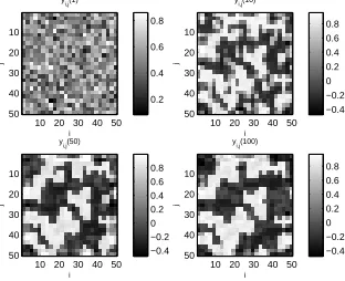
The observation variable was set to be yi,j = xi,j. Some
snapshot patterns are shown in Fig.(8). With these parameters, the system is actually in a chaotic regime with a maximal
Lyapunov exponent λ1 = 0.016046, which was calculated
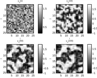
from the spatial average values of the snapshots by using a numerical algorithm proposed by Rosenstein, Collins, and De Luca (1993). A double-level wavelet decomposition was applied to the data with Haar wavelets as a basis, the obtained coarse snapshots are shown in Fig. (9) at the first level and Fig. (10) at the second level. For the coarser data, the numerically
calculated maximal Lyapunov exponent is 0.016046 at the
first scale which is the same as the one calculated from the
finer data and0.018615. This shows that chaotic systems are
essentially self-similar and multiscale.
In the identification, the same set of 200observation pairs
randomly selected among the coarse data set were used. The neighbourhood was set to be the nearest four sites, that is,
(i, j−1),(i, j+ 1),(i−1, j), and(i+ 1, j)and the time lag
was set to be 2. The identified model is listed in Table (II) The model predicted snapshots of the identified model are plotted in Fig.(11) and the maximal Lyapunov exponent for
the model predicted data is 0.014055which is quite close to
the value 0.016946. The obtained model in Table (II) was
also used to produce predictions for the system behaviour at a finer scale and a coarser scale. The results are shown in Figs. (12) to (14). The corresponding maximal Lyapunov exponents are 0.014055 and 0.014055 for the finer scale predictions
with and without high frequency details, and 0.015152 for
the coarser scale prediction. From the simulation results it can be observed that the identified model is able to reproduce the chaotic behaviour at different scales of the underlying spatio-temporal system with high performance.
V. CONCLUSIONS
A novel approach to the multiscale identification of spatio-temporal dynamics has been introduced. It has been demon-strated that the wavelet multiresolution analysis provides a powerful approximation tool for the multiscale representation of the spatio-temporal dynamics. It is also shown that it is possible to extract a system model at some coarse scale, which can then be used to produce predictions for the system behaviour at different scales with or without high frequency
i
j
y
i,j(1)
10 20 30 40 50 10 20 30 40 50 0.2 0.4 0.6 0.8 i j y i,j(10)
10 20 30 40 50 10 20 30 40 50 −0.5 0 0.5 i j y i,j(50)
10 20 30 40 50 10 20 30 40 50 −0.5 0 0.5 i j y i,j(100)
[image:10.595.50.315.102.211.2]10 20 30 40 50 10 20 30 40 50 −0.5 0 0.5
Fig. 8. Example 2: Some snapshots of data (att= 1,10,50, and100)
i
j
y
i,j(1)
5 10 15 20 25 5 10 15 20 25 0.5 1 1.5 i j y i,j(10)
5 10 15 20 25 5 10 15 20 25 −1 −0.5 0 0.5 1 1.5 i j y i,j(50)
5 10 15 20 25 5 10 15 20 25 −1 −0.5 0 0.5 1 1.5 i j y i,j(100)
[image:10.595.360.517.106.235.2]5 10 15 20 25 5 10 15 20 25 −1 −0.5 0 0.5 1 1.5
Fig. 9. Example 2: Some snapshots of data (att= 1,10,50, and100) at the first coarse scale
i
j
yi,j(1)
2 4 6 8 10 12 2 4 6 8 10 12 1.5 2 2.5 i j
yi,j(10)
2 4 6 8 10 12 2 4 6 8 10 12 −1 0 1 2 3 i j
yi,j(50)
2 4 6 8 10 12 2 4 6 8 10 12 −1 0 1 2 3 i j
yi,j(100)
2 4 6 8 10 12 2 4 6 8 10 12 −1 0 1 2 3
Fig. 10. Example 2: Some snapshots of data (att= 1,10,50, and 100) from the second-level wavelet decomposition
i
j
y
i,j(1)
5 10 15 20 25 5 10 15 20 25 0.5 1 1.5 i j y i,j(10)
5 10 15 20 25 5 10 15 20 25 −0.5 0 0.5 1 1.5 i j y i,j(50)
5 10 15 20 25 5 10 15 20 25 −0.5 0 0.5 1 1.5 i j y i,j(100)
5 10 15 20 25 5 10 15 20 25 −0.5 0 0.5 1 1.5
[image:10.595.360.516.278.403.2] [image:10.595.361.512.455.581.2]i
j
y
i,j(1)
10 20 30 40 50 10 20 30 40 50 −0.5 0 0.5 1 i j y i,j(10)
10 20 30 40 50 10 20 30 40 50 −0.5 0 0.5 1 i j y i,j(50)
10 20 30 40 50 10 20 30 40 50 −0.5 0 0.5 1 i j y i,j(100)
[image:11.595.99.255.102.230.2]10 20 30 40 50 10 20 30 40 50 −0.5 0 0.5 1
Fig. 12. Example 2: Some snapshots of reconstructed outputs (at t = 1,10,50, and100) with details at the original scale using the identified coarse model
i
j
y
i,j(1)
10 20 30 40 50 10 20 30 40 50 0.2 0.4 0.6 0.8 i j y i,j(10)
10 20 30 40 50 10 20 30 40 50 −0.4 −0.2 0 0.2 0.4 0.6 0.8 i j y i,j(50)
10 20 30 40 50 10 20 30 40 50 −0.4 −0.2 0 0.2 0.4 0.6 0.8 i j y i,j(100)
10 20 30 40 50 10 20 30 40 50 −0.4 −0.2 0 0.2 0.4 0.6 0.8
Fig. 13. Example 2: Some snapshots of reconstructed outputs (at t = 1,10,50, and100) without details at the original scale using the identified coarse model
information of the original dynamics. The proposed approach can not only generate a simple, effective model for the system but can significantly reduce the noise contained in the signals. Simulation results were included to demonstrate that the new wavelet-based identification procedure can produce excellent models with a very good model predictive performance.
ACKNOWLEDGMENT
The authors gratefully acknowledge financial support from EPSRC (UK).
REFERENCES
[1] Aderson, T. W. and Taylor, J. B., (1979) Strong consistency of the least squares estimates in dynamic models, The annals of Statistics, Vol. 7, No.3, pp. 484-489.
[2] Billings,S. A., Chen, S., and Kronenberg, M. J. (1988) Identification of MIMO nonlinear systems using a forward-regression orthogonal estima-tor,Int. J. Contr., Vol. 49, No. 6, pp. 2157-2189, 1989.
[3] Billings, S. A., Guo, L. Z., and Wei, H. L., (2006) Identification of coupled map lattice models of spatio-temporal patterns using wavelets,
Int. J. Syst. Sci., Vol. 37, No. 14-15, pp.1021-1038.
[4] Bindal, A., Khinast, J. G., and Ierapetritou, M. G., (2003) Adaptive multiscale solution of dynamical systems in chemical processes using wavelets,Computers and Chemical Engineering, Vol. 27, pp. 131-142. [5] Car, R. and Parrinello, M., (1985) Unified approach for molecular
dynamics and density-functional theory,Physical Review Letters, Vol. 55, No. 22, pp. 2471-2474.
[6] Chaudhari, A., Yan, C., and Lee, S. L., (2003) Multifractal scaling analysis of autopoisoning reaction over a rough surface,Journal of Physics A: Mathematical and General, Vol. 36, pp. 3757-3772.
i
j
y
i,j(1)
2 4 6 8 10 12 2 4 6 8 10 12 1.5 2 2.5 i j y i,j(10)
2 4 6 8 10 12 2 4 6 8 10 12 −1 0 1 2 3 i j y i,j(50)
2 4 6 8 10 12 2 4 6 8 10 12 −1 0 1 2 3 i j y i,j(100)
[image:11.595.361.512.103.231.2]2 4 6 8 10 12 2 4 6 8 10 12 −1 0 1 2 3
Fig. 14. Example 2: Some snapshots of reconstructed outputs (at t = 1,10,50, and100) at second coarse scale using the identified coarse model
[7] Chui C. K., (1992)An Introduction to Wavelets, San Diego: Academic Press, Inc.
[8] Coca, D. and Billings, S. A., (2001) Identification of coupled map lattice models of complex spatio-temporal patterns,Phys. Lett., A287, pp. 65-73. [9] Coca, D. and Billings, S. A., (2002) Identification of finite dimensional models of infinite dimensional dynamical systems,Automatica, Vol. 38, pp. 1851-1856.
[10] E., W. N., Engquist, B., Li, X., Ren, W., and Vanden-Eijnden, E., (2006) The heterogeneous multiscale method: A review, preprint, http://www.math.princeton.edu/multiscale/review.pdf
[11] E., W. N., and Engquist, B. (2003) Multiscale modelling and Computa-tion,Notices of the AMS, Vol. 50, No.9, pp.1062-1070.
[12] Eck, C., (2004) Analysis of a two-scale phase field model for liquid-solid phase transitions with equiaxed dendritic microstructures,Multiscale Modeling and Simulation, Vol. 3, No. 1, pp. 28-49.
[13] Feldmann, A., Gilbert, A. C., Willinger, W., and Kurtz, T. G., (1998) The changing nature of network traffic: scaling phenomena, Computer Communications Review, Vol. 28, No. 2, pp. 5-29.
[14] Kaneko, K., (1989) Spatiotemporal chaos in one- and two-dimensional coupled map lattices,Physica, D37, pp. 60-82.
[15] Korenberg, M., Billings, S. A., Liu, Y. P., and Mcilroy, P. J., (1988) Orthogonal parameter estimation algorithm for non-linear stochastic sys-tems, Int. J. Contr., Vol. 48, No.1, pp. 193-210.
[16] Guo, L. Z. and Billings, S. A., (2006) Identification of partial differential equation models for continuous spatio-temporal dynamical systems,IEEE Trans. Circuits and Systems – II: Express Briefs, Vol. 53, No. 8, pp. 657-661.
[17] Guo, L. Z., Billings, S. A., and Wei, H. L., (2006) Estimation of spatial derivatives and identification of continuous spatio-temporal dynamical systems,Int. J. Contr., Vol.79, No. 9, pp. 1118-1135.
[18] Guo, L. Z. and Billings, S. A., (2007) A modified orthogonal forward regression least-squares algorithm for system modelling from noisy regressors,Int. J. Contr., Vol.80, No. 3, pp. 340-348.
[19] Huerta, R., Rabinovich, M. I., Abarbanel, H. D. I., and Bazhenov,M., (1997) Spike-train bifurcation scaling in two coupled chaotic neurons,
Physical Review E, Vol. 55, No. 3, pp. R2108-2110.
[20] Littlewood, D. J. and Maniatty, A. M., (2005) Multiscale modelling of crystal plasticity in AL 7075-T651, inProceedings of VIII International Conference on Computational Plasticity, Barcelona, Spain, pp. 618-621. [21] Lorenz, E. N., (1996) Predictability: a problem partly solved, inProc.
Seminar on Predictability, Vol. 1, ECMWF, Reading, Berkshire, UK, pp. 1-18.
[22] Louie, M. M. and Kolaczyk, E. D., (2006) A multiscale method for disease mapping in spatial epidemiology,Statistics in Medicine, Vol. 25, No. 8, pp. 1287-1308.
[23] Mandelbrot, B. B., (1967) How long is the coast of Britain? Statistical self-similarity and fractional dimension,Science, Vol. 156, pp. 636-638. [24] McSharrya, P. E., Ellepolab, J. H., von Hardenberga, J., Smitha, L. A., and Kenning, D., (2002) Spatio-temporal analysis of nucleate pool boiling: identification of nucleation sites using non-orthogonal empirical functions,Int. J. Heat & Mass Transfer, Vol. 45, No. 2, pp. 237-253. [25] Muller-Buschbaum, P., Bauer, E., Pfister, S., Roth, S. V., Burghammer,
[image:11.595.98.254.291.418.2][26] Rosenstein, M. T., Collins, J. J., and De Luca, C. J., (1993) A practical method for calculating largest Lyapunov exponents from small data sets,
Physica, D65, pp. 117-134.
[27] Schwartz, I. B., Morgan, D. S., Billings, L., Lai, Y. C., (2004) Multi-scale continuum mechanics: From global bifurcations to induced high-dimensional chaos,Chaos, Vol. 14, No. 2, pp. 373-386.
[28] Voss, H., Bunner, M. J. Bunner, and Abel, M., (1998) Identification of continuous, spatiotemporal systems,Physical Review E, Vol. 57, No.3, pp. 2820-2823.