The Impact of Walking Time on U Shaped Assembly Line Worker Allocation Problems

(1)

www.ej.eng.chula.ac.th ENGINEERING JOURNAL : VOLUME 14 ISSUE 2 ISSN 0125-8281 : ACCEPTANCE DATE, APR. 2010

53

T

HE

I

MPACT OF

W

ALKING

T

IME

ON

U

-SHAPED

A

SSEMBLY

L

INE

W

ORKER

A

LLOCATION

P

ROBLEMS

Ronnachai Sirovetnukul and Parames Chutima*

Department of Industrial Engineering, Faculty of Engineering,

Chulalongkorn University, Bangkok, Thailand 10330

E-mail : [email protected] and [email protected]*

ABSTRACT

The one-piece flow manufacturing line of single and customized products is

usually organized as a U-shaped assembly layout. In this study, the

characteristics of a single U-line are described and modeled. The worker

allocation problem is hierarchically concerned with the task assignment into a

U-line and allocate task to workers in sequence. Several products are

assembled in 7-task to 297-task problems, and each problem is performed

with a given cycle time. The primary purpose is to identify the impact of

walking time on both symmetrical and rectangular U-shaped assembly layouts.

The minor purpose is to compare the number of workers between two fixed

layouts. Coincidence algorithm demonstrates clarifying solutions. To respond

to two previous aims, the primary objective function of a number of workers is

used. Finally, with the Pareto-optimal frontier between the deviation of

operation times of workers and the walking time, its computational study is

exemplified to identify good task assignment and walking path.

KEYWORDS

(2)

54 ENGINEERING JOURNAL : VOLUME 14 ISSUE 2 ISSN 0125-8281 : ACCEPTANCE DATE, APR. 2010 www.ej.eng.chula.ac.th

I . Introduction

Traditionally, a straight assembly line is suitable for mass production. In the circumstance of product variety, an assembly line is replaced with the U-shaped line. The decision to transform straight-line assembly systems to U-shaped assembly line systems constitutes a major layout design change and investment for assembly operations. Proponents of the lean manufacturing and just-in-time (JIT) philosophies assert that U-shaped assembly systems offer several benefits over traditional straight-line layouts [1] especially an improvement in labor productivity. U-lines have become popular in order to obtain the main benefits of smoothed workload, multi-skilled workforce and other principles of the JIT philosophy. Many researchers agree that U-lines are one of the most important components for a successful implementation of JIT production systems [2],[3]. The U-line is equivalent to the straight line for any allocation of tasks or machines to workers so long as a worker does not work together with other stations (i.e. no crossing loop). The number of workers required on a U-line is never more than that required on a straight U-line [1]. However, a worker can be either in the similar line or across from the front line to the back line or vice versa. Thus, the historical results of a number of workers from the straight line balancing cannot be used due to lack of the addition of walking time. Walking time is also negligible for U-line balancing problems in most papers [4] - [8] but walking time should be considered as workers follow circular paths and walk on the beginning (front), the ending (back) and the middle (side) U-line to complete their tasks. There are two research gaps to be filled in this paper. The first research question is whether and how much the appropriate walking time between tasks should be considered in the U-line instead of the ignorance as often modeled in the straight line problem. Secondly, the research question is whether different fixed U-shaped layouts affect the number of workers. This paper remarks that adding the walking time at the early percentage of average processing time significantly increases the number of workers. The line balancing problem can be replaced with the worker allocation problem if a single worker can handle multiple tasks. Hierarchically after solving the minimum number of workers, the rest of multi-objective coincidence algorithm for tackling the U-shaped worker allocation problem is developed in this research. The objective of the described study is to allocate workers in single U-shaped assembly line problems having manually operated machines by determining the average processing time percentage.

The structure of this paper is as follows. In Section II, previous related literature is reviewed. Section III describes the physical and mathematical models. This model is primarily used to minimize a number of workers needed to perform tasks. Secondly, dual objectives are to minimize the deviation of operation times of workers and their walking time simultaneously with the development of evolutionary algorithm. The combinatorial optimization with the coincidence algorithm and its numerical example are explained in Section IV. Experimental results are presented in Section V. The last section concludes the work and discusses the potential future work.

Il. Literature Review

2.1 U-shaped assembly line balancing problems

(3)

55

Miltenburg and Wijngaard [10] were the first to compare a U-shaped line with a straight line. There are many papers that reveal advantages of the U-shaped layout over the linear layout [1],[6],[11],[12],[13] Cheng et al. [1] found collectively that the benefits and factors favoring U-lines are better volume flexibility, worker flexibility, number of workstations, material handling, visibility and teamwork, and rework. Miltenburg [14] analyzes the U-line facility problem where a multi-line station may include tasks from two adjacent U-lines. To solve the problem, a dynamic programming approach is used. Sparling [15] also investigates the multiple U-line problems and presents several heuristic approaches to solve the N U-line facility problem. More complex U-lines, which are not a single or simple U-line, are named multi-lines in a single U, double-dependent U-lines, embedded U-lines, figure-eight-pattern U-lines, and multi-U-line facility [16]. Travel time between tasks are hardly considered; however, at present only Miltenburg [3] in the issue of line balancing and Shewchuk [17] in the issue of worker allocation consider walking time. Miltenburg [3]’s 10-task problem of a single U-line was studied hierarchically in USALBP-1. It gives us the optimal number of workstations with walking distance (one unit for adjacent machines (at the same row) and two units for opposite machines). The paper of Shewchuk studied the same problem of 5-20 machines (or tasks) with walking time (one second for adjacent machines (same row) and two seconds for opposite machines). This research relaxes Shewchuk’s assumption that does not guarantee minimum walking times on page 3,489 [17]. It will be studied in the following experiments in this research. However, it did not refer to the input of the precedence graph. As a result, its optimum number of workstations with walking time cannot be compared.

2.2 Data sets of U-shaped assembly line balancing problems

The well-known Talbot’s data set based on 12 precedence networks with 8-111 tasks, each of which is combined with several cycle times is adapted to build a total of 64 instances [18]. Miltenburg [14] noted that U-line problem sets with more than 26 tasks may be too difficult to solve in more restricted constraints. However, Scholl’s data sets are composed of 168 instances with 25-297 tasks [19]. All instances form the combined data set with 269 instances. Complete descriptions of all data sets are given in chapter 7.2 of Scholl [19] and can be downloaded from http://www.assembly-line-balancing.de. These sets are used for testing ULINO which is applied directly to the U-shaped Assembly Line Balancing Problem of type I (UALBP-I)

2.3 U-shaped worker allocation problems

(4)

2.4 Worker allocation objective functions

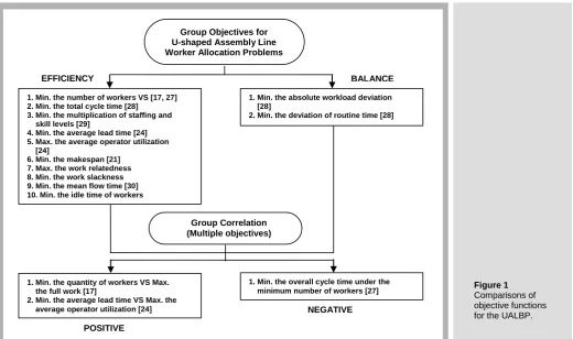
Historical single and multiple objective functions have been studied by several researchers. Efficiency and balance performance measures influencing just-in-time manufacturing (especially in UALBP) are reviewed and shown in Figure 1. In the study of decision making, terms such as multiple objectives, multiple attributes, and multiple criteria are used interchangeably. Multiple objectives decision making consists of a set of conflicting goals that cannot be achieved simultaneously. The motivation to consider the problem of generating the efficient set of the worker allocation problem comes from the variety of industrial cases where the criteria are related to the minimum number of workstations, smoothed workload in a sense of equity, and minimum walking time to save the space needed for the actual size of a U-shaped line and shorten distance for communication between workers.

Authors(Year) Problem

description Problem set Objectives

Walking

time Solution techniques

Miltenburg and

Wijngaard (1994) [10] Single model

Up to 11 tasks

Up to 111 tasks Number of workstations No

DP formulation RPWT-based heuristic Miltenburg and

Sparling (1995) [21] Single model Up to 40 tasks Number of workstations No

DP-based exact algorithm Depth-first and breath-first B&B Ajenblit and

Wainwright (1998) [4] Single model Up to 111 tasks

Number of workstations and

workload balance No Generic algorithm

Miltenburg (1998) [14]

U-line facility with several individual U-lines

Individual U-lines with up to 22 tasks

idle time in a single station No DP-based exact algorithm Sparling and

Miltenburg (1998) [15] Mixed model Up to 25 tasks Number of workstations No Heuristic Urban (1998) [16] Single model Up to 45 tasks Number of workstations No IP formulation Scholl and Klein

(1999) [7] Single model Up to 297 tasks Number of workstations No B&B-based heuristic Miltenburg (2001) [3] Single model 10 tasks Number of workstations Yes* ILP and DP formulation

Hwang and Katayama

(2008) [13] Mixed model 19, 61 and 111 tasks

workload variation No Genetic algorithm

Shewchuk (2008) [16]** Lean single U-_lines Up to 20 tasks Number of workstations and _{maximize full work} Yes Heuristic

This research study

Single&mixed model with several single U-lines

Up to 297 tasks

Number of workstations, workload smoothness, and walking time

Yes Multi-objective evolutionary algorithm

[image:4.595.41.449.59.276.2]

*Walking time is set at one unit for adjacent tasks at the same row and two units for opposite tasks. **Shewchuk [16] did not use the standard problems of precedence constraints and given cycle time.

Table 1 Summary of the papers conducted on single U-shaped assembly lines.

1. Min. the number of workers VS [17, 27] 2. Min. the total cycle time [28]

3. Min. the multiplication of staffing and skill levels [29]

4. Min. the average lead time [24] 5. Max. the average operator utilization [24]

6. Min. the makespan [21] 7. Max. the work relatedness 8. Min. the work slackness 9. Min. the mean flow time [30] 10. Min. the idle time of workers

1. Min. the absolute workload deviation [28]

2. Min. the deviation of routine time [28]

1. Min. the quantity of workers VS Max. the full work [17]

2. Min. the average lead time VS Max. the average operator utilization [24]

1. Min. the overall cycle time under the minimum number of workers [27]

EFFICIENCY BALANCE

POSITIVE

NEGATIVE Group Objectives for

U-shaped Assembly Line Worker Allocation Problems

[image:4.595.39.560.485.793.2]

Group Correlation (Multiple objectives)

(5)

57

2.5 Solution techniques

Using exact solution for small size problems of U-shaped assembly line balancing is studied in some papers. It is well known that traditional assembly line balancing problems (ALBP) fall into the NP-hard class of combinatorial optimization problems [8] As a result of the problem complexity, it is difficult to find an optimal solution in polynomial time. Since both the MALBP and the UALBP are subsets of the ALBP, they are also NP-hard. Therefore, mathematical methods that evaluate the entire solution space are not suitable for large sized problems and heuristics need to be employed in order to efficiently search the solution space. Since last two decades there has been many multiple objective evolutionary algorithms as mentioned by Chutima and Pinkoompee [31]. However, the COINcidence algorithm [26] is preferable to Non-dominated Sorting Genetic Algorithm (NSGA-II) [32] due to the additional use of negative knowledge that renders faster convergence speed and less CPU time. The details of COIN are later described in Section VI.

III. Model Configurations

3.1 Problem development

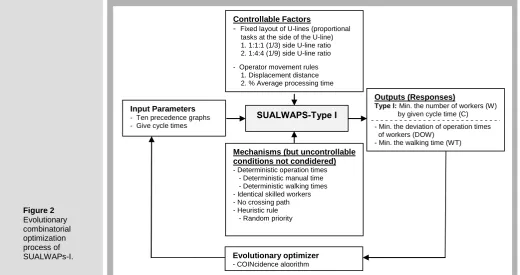
[image:5.595.42.563.518.793.2]

The Just-in-time (JIT) production system has been adopted extensively in today’s manufacturing industries such as the apparel industry to meet production demands. A U-shaped production line can be described as a special type of cellular manufacturing used in JIT production systems. In recent decades, many apparel manufactures have installed several production systems on their apparel assembly lines such as the traditional progressive bundle system and the automated unit production system [33]. The assembly line to be studied in this paper is a modular production system (or a single U-line). There are no automated processing machines in the production system. After each worker operates an item at a machine, a worker walks with several patterns such as a circular loop, a rectangular loop, or a straight-line loop and takes it to the next machine and at the end of each intra loop. Generally a worker hands it over to the adjacent worker along the sequence of U-line. From some of the sample companies, there is no equity of workload although line efficiency has been continuously improved. In practice, most companies manage the assembly line problem of type F (given number of workstations and given cycle time) and improve line efficiency by avoiding the complexity of the problem. However, this paper studies the problem of type I: the minimum number of workstations at given cycle times. The evolutionary combinatorial optimization process of Single U-shaped Assembly Line Worker Allocation Problems of type I (SUALWAPs-I) minimizing the number of workers given a target cycle time is illustrated in Figure 2.

Figure 2 Evolutionary combinatorial optimization process of SUALWAPs-I.

Controllable Factors

- Fixed layout of U-lines (proportional tasks at the side of the U-line) 1. 1:1:1 (1/3) side U-line ratio 2. 1:4:4 (1/9) side U-line ratio

- Operator movement rules 1. Displacement distance 2. % Average processing time

Input Parameters - Ten precedence graphs - Give cycle times

Mechanisms (but uncontrollable conditions not condidered) - Deterministic operation times - Deterministic manual time - Deterministic walking times - Identical skilled workers - No crossing path - Heuristic rule - Random priority

Evolutionary optimizer - COINcidence algorithm

SUALWAPS-Type I

Outputs (Responses)

Type I: Min. the number of workers (W) by given cycle time (C)

- Min. the deviation of operation times of workers (DOW)

(6)

3.2 Input parameters

In any time period, the number of jobs is deterministic and job arrivals come from not only new customer orders but also remaining jobs from the previous planning period that were not completed. Each job is an entity worked on many tasks. No job priority (i.e. no preemption job) constraint is allowed: that is, each job is allowed to start its processing whenever it is ready. These jobs are sorted by the daily production order excluding the sequencing problem. The ten standard precedence graphs (7-task to 297-task assembly networks) and various cycle times (the time which is available at each station to perform all the tasks assigned to the station) are input in U-shaped assembly line worker allocation problems [26]. They are referred to in column one and two of Table 4 in Section 3.5. Given precedence graphs for an assembly line are produced from the process of making intermediate parts in the final assembly line.

3.3 Characteristics of a single assembly U-line

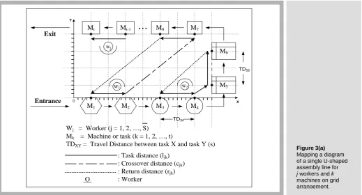
Although there are many types of lines, the configuration of this study is a single U-shaped assembly line only. The U-line arranges machines or tasks around a U-U-shaped line in the order in which production tasks are serial. The sequence of tasks on the U-line is not fixed, making it possible to reallocate tasks to different U-line locations. Thus, the assignment of tasks to line locations can be altered. The system is one-piece flow manufacturing moving one piece at a time between tasks within a U-line. One floating worker supervises both the entrance and the exit of the line. The task efficiency is proportional to the worker’s performance. Machine-work is not separated from worker-work. Standard operation charts specify exactly how all work is done. Workers can be reallocated periodically when production requirements change (or cycle time changes). This requires workers to have multi-functional skills to operate several different machines or tasks. It also requires workers to work standing up and walking because they need to operate at different locations. Whenever a worker arrives at a task, one performs any needed tasks at the task location, and then walks to the next task. Following the last task of a path, the worker returns to the starting point and works or waits for the start of the next cycle. The characteristics of the single U-shaped assembly line worker allocation problem of type I are shown in Figure 3(a).

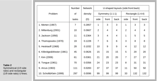
The U-line layouts illustrated in Table 2 are configured with symmetrical and rectangular shapes at the side ratios of 1/3 (1:1:1) and 1/9 (1:4:4), respectively. They are representative enough for the workable single U-line. The line consists of M

Figure 3(a) Mapping a diagram of a single U-shaped assembly line for j workers and k

machines on grid arrangement.

Mt Mt-1 M8 M7

M1 M2 M3 M4

M6

M5

Entrance Exit

Wj = Worker (j = 1, 2, …, S)

Mk = Machine or task (k = 1, 2, …, t)

TDXY = Travel Distance between task X and task Y (s)

: Task distance (ljk)

: Crossover distance (cjk)

: Return distance (rjk)

O : Worker

w1

wj

...

0 _X

Y

w2

TD34

[image:6.595.40.560.449.729.2]

(7)

59

machines or k tasks in a U-shape arrangement with the side of Modd or Meven. Walking distance and travel speed of each worker are considered into walking time in section 3.5. The values of network density (D) are also shown in column III of Table 2. Network density, a characteristic which measures the strength of this relationship, has been found to be an important factor in influencing heuristic performance in previous investigations of the line balancing problem [18]. The density of the assembly network is defined as the ratio ofD, Let d denote the total number of precedence relations in the precedence graph, and N denote the number of task on a U-line. Then, D = 2d/[N(N - 1)] where D1.0. Values of D close to 1 indicate a highly interconnected network with fewer alternatives available for assigning tasks to a work station. Values of D close to 0 indicate relatively fewer precedence relationships, and more opportunities for assigning tasks to a work station.

3.4 Mathematical model

In this section, a mathematical model for solving the worker allocation problem is described. The symbols used are listed and explained in the next section.

3.4.1 Notation used

The notation used in this section can be summarized as follows:

Indices

j = index on workers

k = index on tasks

Parameters

t = number of tasks in the U-line

C = given cycle time

P = {( , ) :k l task kmust be completed before task lcan begin}– precedence

constraints

k

t = time to complete manual task at task k

 = coefficient of walking time

Variables

S = number of workers in the U-line

jk

[image:7.595.38.561.200.470.2]

C _{= cycle time at task}kassigned to worker j Table 2

Symmetrical (1/3 side ratio) and rectangular (1/9 side ratio) U-lines.

Number Network U-shaped layouts (side:front:back)

Problem of density Symmetry (1:1:1) Rectangle (1:4:4)

tasks (D) side front back side front back

1. Merten (1967) 7 0.2857 1 3 3 1 3 3

2. Miltenburg (2001) 10 0.0667 2 4 4 2 4 4

3. Jackson (1956) 11 0.2364 3 4 4 1 5 5

4. Thomopoulos (1970) 19 0.1228 7 6 6 3 8 8

5. Heskiaoff (1968) 28 0.1032 10 9 9 4 12 12

6. Kilbridge&Wester (1961) 45 0.0626 15 15 15 5 20 20

7. Kim (2006) 61 0.0361 21 20 20 7 27 27

8. Tongue (1961) 70 0.0356 24 23 23 8 31 31

9. Arcus (1963) 111 0.0283 37 37 37 11 50 50

(8)

m = minimum number of workers

jk

l _{= task distance at task}kassigned to worker j

jk

c _{= crossover distance at task}kassigned to worker j

jk

r _{= return distance at task}kassigned to worker j

jk

T = task time at task kassigned to worker j

jk

WT = walking time at task kassigned to worker j

Decision variables

   

1 if task k is located on front of line and assigned to worker j 0 otherwise

jk

x

1

0

if task k is located on back of line and assigned to worker j otherwise

   

jl y

    jl

x 1 if task l is located on front of line and assigned to worker j

0 otherwise

1

0

if task l is located on back of line and assigned to worker j otherwise

   

jl y

1

0 j z  



if worker j is used otherwise

3.4.2 Model formulation

This section identifies the minimum number of workers (workstations) in Eq. (1) required in the U-line to obtain the optimum of dual objectives. Besides aiming to increase productivity (minimizing the number of workers or the cycle time), some other goals are important for the addition of high productivity achievements, i.e., a sense of equity among workers and the shortest travel path. Hierarchically both objective functions are calculated accordingly in the same unit of time from Eq. (2), (3), and (4). An ineffective allocation of workers to tasks and machines would yield long idle times (imbalance workload) and long walking time.

Then select x_jk,y_jk,z_j to,

(ILP) Minimize



S_j_₁z_j (1)

After computing the minimum number of workers in the first step, it is necessary to evaluate and minimize the deviation of operation times of workers (DOW) and the walking time (WT) as seen in Section 3.4.2.1 with Pareto-optimal frontier.

3.4.2.1 Objective functions

I. Min. the deviation of operation times of workers (DOW)

DOW =

2

1 1( )

S t

jk

j k C C

m

  

 

(2)

Cycle Time (C_jk) = Task Time (T_jk) + Walking Time (WT_jk) (3)

(U-Worker Balancing) (U-line Balancing)

II. Min. the walking time (WT)

WT 

 

s_j_₁ _kt_₁



l_jkc_jkr_jk



(4)

3.4.2.2 Constraints

Subject to:

(9)

61



_j(S j 1)(x_jkx_jl)0 for all

 

k l, P (6)

( 1)( _jl _jk) 0

j S j y y 



for all

 

k l, P (7)

x_jk,y_jk,z_j 

 

0,1 for all j, k (8)

The first constraint in Eq. (5) ensures that every task is located on the front or back of the line and is assigned to one worker. The next constraint in Eq. (6) ensures that the precedence constraints are satisfied for each task assigned to the front of the line. The following constraint in Eq. (7) does the same for the tasks of the equation (6) assigned to the back of the line. In other words, constraint (6) enforces task sequence assigned on the U-line by a set of ordered pairs of tasks reflecting the precedence relationships; for example, P = (3,1), (5,10) and (6,9) is the ordered pair of Miltenburg’s 10-task problem indicating task k precedes task l. X_jkor/and Xjl is 1 when worker jdoes

task k or/and task l. Otherwise, its value is 0 or their values are 0. Constraints (7) is the same, but is reversed because task on the U-line can be also assigned at the back line. The variables of x, y, and z are binary solution in Eq. (8). However, Miltenburg [3] does not take walking distance into account and may not find the best U-line design. Thus, the last constraint of walking time in Eq. (9) is essential to complete the worker allocation problem. The constraint proves that the sum of the manual task times for the tasks in each worker in the first term and the total walking distance in the second term does not exceed the cycle time, C. The coefficient of walking time( ) is varied by TDXY in Figure 3(a)

or the percentage of Average Processing Time (APT) from one task to another task. The average processing time is defined as APT =



t_k_₁t_k/t.



   

W_j _jT_jk _j(l_jk+ c_jk+ r_jk) C

for all j,k (9)

3.4.2.3 Illustrative example

For Miltenburg’s 10-task problem, the precedence graph is (3,1), (5,10) and (6,9) and taskManual time is 13, 24, 32, 42, 54, 64, 73, 82, 92, 102. Suppose that Task Sequence (TS) on the U-line is -1_7_2_-10_6_5_8_9_4_3. This means task 1, which is assigned to the back location of the line. Then task 7 is assigned to the front location on the front of the line. Finally, the rest of task sequence is assigned. The sequence is feasible because the precedence constraints are satisfied with five tasks on the front and five tasks on the back. Suppose C = 10 seconds, and  = 1 at 35% average processing time. Then the assigned task to workers is [-1_7]_[2_-10]_[6_5]_[8_9_4]_[3] shown in Figure 3(b). Tasks 1 and 7 are in the worker 1 and the manual times (T_jk) of T11 and T17 are 3 and 3,

respectively. From Eq. (3), W₁(T₁₁T₁₂)  WT₁k;where WT1k l11l12c11r12.

Thus, W₁       (3 3) 1 (0 0 2 2) 10seconds. After that, the cycle times (C_jk) of worker 2 to worker 5 are computed as the same.

7

2

6

5

8

9

4

3

10

1 Exit

Entrance

Front

Back

Figure 3(b)

[image:9.595.38.558.593.792.2]

(10)

3.4.3 Assumptions

In this study, the SUALWAPs-I is subjected to the following assumptions:

 A U-line comprises inexpensive and small non-automated machines. Several identical machines may be found and machines are enough to be allocated in a single U-line;

 Machines or tasks are located via a grid arrangement with the same distance of %APT between adjacent task locations in the same row. For other non-adjacent task locations, the walking distance is calculated by the displacement of Euclidean distance;

 Trained homogeneous skilled workers have the same efficiency and multi- functional skills and are able to operate any processes or machines. They walk in a circle inside the U-line (also called the zone constraint – machines allocated to each worker must be adjacently located within a loop);

 A worker is assigned to one station (or one loop) only;

 All parameters and variables such as processing times and walking times are deterministic (known and constant);

 The completion time of a machine or task summed with many subordinate tasks is known and a task cannot be split between two or more workers;

 Precedence relationships of the problem are consistent from model to model. That is, if task

k

precedes task

l

in any model there is no other model where task

l

must precede task

k

. Each unit of products is processed through all tasks in the same precedence order;

 Setup times (assumed to be less than 10% compared with processing time) are negligible. U-lines can be operated as single-model and mixed-model lines where each worker is able to produce any product in any cycle. Consequently, job sequence is regardless at any period;

 The mixed-model task times use the weight of composite demand to transform average task time into the task of a single model. However, a floating worker may be assisted unless task times in some model are feasible;

 Learning effect has no consideration since it is assumed that worker performance runs into steady state already;

The mathematical model of this research is not studied in depth because minimizing the number of workers, DOW and WT at the same time make the exact solution too complex to deal with.

3.5 Determination of walking time

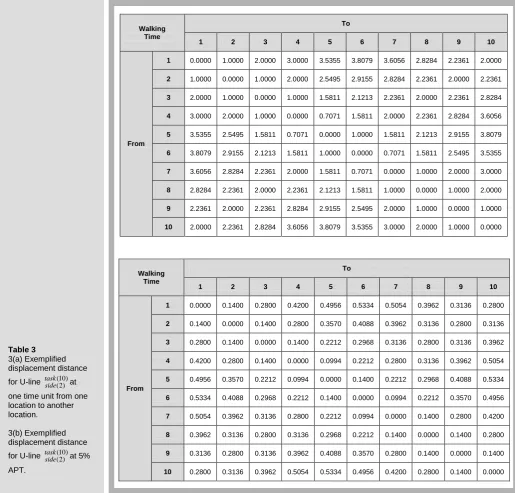
In the previous papers [3], [17], [26] the coefficient of walking time ( ) is required to travel a unit of distance or one time unit. Thus, in this study the adjacent matrix (From-To chart) of walking times under displacement distance for each problem of the symmetrical and rectangular shape is initially constructed at one time unit from one location to another location. Each of the walking times between a pair of tasks is directly proportional to Euclidean distance between locations. The example of walking times for the 10-task problem is shown in Table 3 (a). For example, the displacement gives us a travel distance of 0.7071 distance units (or time units), calculated as the

sum of distance between location (3, 0), (3.5, 0.5)  (3.5 - 3)2(0.5 - 0)2 0.7071,where is a Euclidean distance operator. Note that: Location 1 is assumed to be an origin (0,0).

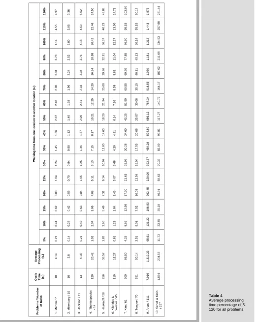
In practice, a worker keeps walking more than one second. However, Balakrishnan et al. [34] assumingly use two values of travel time for each problem instance, (i.e. walking time = the five or ten percentage of Average Processing Times (APT), where APT is the expected value of processing times which is defined as APT



t_k_₁t_k/t;

where tk is task time k and tis the summation of task 1 to k. In this study, the values

(11)

[image:11.595.48.564.140.633.2]

63 Table 3

3(a) Exemplified displacement distance

for U-line task_side(10)₍₂₎ at one time unit from one location to another location.

3(b) Exemplified displacement distance

for U-line task_side(10)₍₂₎ at 5% APT.

Walking Time

To

1 2 3 4 5 6 7 8 9 10

From

1 0.0000 1.0000 2.0000 3.0000 3.5355 3.8079 3.6056 2.8284 2.2361 2.0000

2 1.0000 0.0000 1.0000 2.0000 2.5495 2.9155 2.8284 2.2361 2.0000 2.2361

3 2.0000 1.0000 0.0000 1.0000 1.5811 2.1213 2.2361 2.0000 2.2361 2.8284

4 3.0000 2.0000 1.0000 0.0000 0.7071 1.5811 2.0000 2.2361 2.8284 3.6056

5 3.5355 2.5495 1.5811 0.7071 0.0000 1.0000 1.5811 2.1213 2.9155 3.8079

6 3.8079 2.9155 2.1213 1.5811 1.0000 0.0000 0.7071 1.5811 2.5495 3.5355

7 3.6056 2.8284 2.2361 2.0000 1.5811 0.7071 0.0000 1.0000 2.0000 3.0000

8 2.8284 2.2361 2.0000 2.2361 2.1213 1.5811 1.0000 0.0000 1.0000 2.0000

9 2.2361 2.0000 2.2361 2.8284 2.9155 2.5495 2.0000 1.0000 0.0000 1.0000

10 2.0000 2.2361 2.8284 3.6056 3.8079 3.5355 3.0000 2.0000 1.0000 0.0000

Walking Time

To

1 2 3 4 5 6 7 8 9 10

From

1 0.0000 0.1400 0.2800 0.4200 0.4956 0.5334 0.5054 0.3962 0.3136 0.2800

2 0.1400 0.0000 0.1400 0.2800 0.3570 0.4088 0.3962 0.3136 0.2800 0.3136

3 0.2800 0.1400 0.0000 0.1400 0.2212 0.2968 0.3136 0.2800 0.3136 0.3962

4 0.4200 0.2800 0.1400 0.0000 0.0994 0.2212 0.2800 0.3136 0.3962 0.5054

5 0.4956 0.3570 0.2212 0.0994 0.0000 0.1400 0.2212 0.2968 0.4088 0.5334

6 0.5334 0.4088 0.2968 0.2212 0.1400 0.0000 0.0994 0.2212 0.3570 0.4956

7 0.5054 0.3962 0.3136 0.2800 0.2212 0.0994 0.0000 0.1400 0.2800 0.4200

8 0.3962 0.3136 0.2800 0.3136 0.2968 0.2212 0.1400 0.0000 0.1400 0.2800

9 0.3136 0.2800 0.3136 0.3962 0.4088 0.3570 0.2800 0.1400 0.0000 0.1400

(12)

64 ENGINEERING JOURNAL : VOLUME 14 ISSUE 2 ISSN 0125-8281 : ACCEPTANCE DATE, APR. 2010 www.ej.eng.chula.ac.th W a lk in g t im e f ro m o n e l o c a ti o n t o a n o th e r lo c a ti o n ( s .)

120% 4.9

7 3 .3 6 5 .0 2 2 4 .5 0 4 3 .8 8 1 4 .7 2 1 0 3 .8 0 6 0 .1 7 1 ,5 7 5 2 8 1 .4 4 110 % 4 .5 5 3 .0 8 4 .6 0 2 2 .4 6 4 0 .2 3 1 3 .5 0 9 5 .1 5 5 5 .1 5 1 ,4 4 3 2 5 7 .9 8

100% 4.1

4 2 .8 0 4 .1 8 2 0 .4 2 3 6 .5 7 1 2 .2 7 8 6 .5 0 5 0 .1 4 1 ,3 1 2 2 3 4 .5 3

90% 3.7

3 2 .5 2 3 .7 6 1 8 .3 8 3 2 .9 1 1 1 .0 4 7 7 .8 5 4 5 .1 3 1 ,1 8 1 2 1 1 .0 8

80% 3.3

1 2 .2 4 3 .3 4 1 6 .3 4 2 9 .2 6 9 .8 2 6 9 .2 0 4 0 .1 1 1 ,0 5 0 1 8 7 .6 2 70 % 2 .9 0 1 .9 6 2 .9 3 1 4 .2 9 2 5 .6 0 8 .5 9 6 0 .5 5 3 5 .1 0 9 1 8 .5 6 1 6 4 .1 7

60% 2.4

8 1 .6 8 2 .5 1 1 2 .2 5 2 1 .9 4 7 .3 6 5 1 .9 0 3 0 .0 8 7 8 7 .3 4 1 4 0 .7 2

50% 2.0

7 1 .4 0 2 .0 9 1 0 .2 1 1 8 .2 9 6 .1 4 4 3 .2 5 2 5 .0 7 6 5 6 .1 2 1 1 7 .2 7

40% 1.6

6 1 .1 2 1 .6 7 8 .1 7 1 4 .6 3 4 .9 1 3 4 .6 0 2 0 .0 6 5 2 4 .8 9 9 3 .8 1

35% 1.4

5 0 .9 8 1 .4 6 7 .1 5 1 2 .8 0 4 .2 9 3 0 .2 8 1 7 .5 5 4 5 9 .2 8 8 2 .0 9

30% 1.2

4 0 .8 4 1 .2 5 6 .1 3 1 0 .9 7 3 .6 8 2 5 .9 5 1 5 .0 4 3 9 3 .6 7 7 0 .3 6

25% 1.0

4 0 .7 0 1 .0 5 5 .1 1 9 .1 4 3 .0 7 2 1 .6 3 1 2 .5 4 3 2 8 .0 6 5 8 .6 3

20% 0.8

3 0 .5 6 0 .8 4 4 .0 8 7 .3 1 2 .4 5 1 7 .3 0 1 0 .0 3 2 6 2 .4 5 4 6 .9 1

15% 0.6

2 0 .4 2 0 .6 3 3 .0 6 5 .4 9 1 .8 4 1 2 .9 8 7 .5 2 1 9 6 .8 3 3 5 .1 8

10% 0.4

1 0 .2 8 0 .4 2 2 .0 4 3 .6 6 1 .2 3 8 .6 5 5 .0 1 1 3 1 .2 2 2 3 .4 5

5% 0.2

1 0 .1 4 0 .2 1 1 .0 2 1 .8 3 0 .6 1 4 .3 3 2 .5 1 6 5 .6 1 1 1 .7 3 Ave ra g e P ro c e s s in g (s .) 4 .1 4 2 .8 4 .1 8 2 0 .4 2 3 6 .5 7 1 2 .2 7 8 6 .5 0 5 0 .1 4 1 ,3 1 2 .2 3 2 3 4 .5 3 Cyc le T im e (s .)

10 10 13 120 256 110 600 251 ₇,91

[image:12.595.41.568.83.739.2]

(13)

65

IV. Multiple Objective Coincidence Algorithm

4.1 Proposed algorithm

Wattanapornprom et al. [35] developed a new effective evolutionary algorithm called

combinatorial optimization with coincidence (COIN) originally aiming to solve traveling

salesman problems. Several benchmarks are compared to the experiment of Robles et al. [36]. The idea is that most well-known algorithms such as Genetic Algorithm (GA) search for good solutions by sampling through crossover and mutation tasks without much exploitation of the internal structure of good solution strings. This may not only generate large number of inefficient solutions dissipated over the solution space but also consume long CPU time. In contrast, COIN considers the internal structure of good solution strings and memorizes paths that could lead to good solutions. COIN replaces high computation time of crossover and mutation tasks of GA and employs a joint probability matrix as a means to generate neighborhood solutions. It prioritizes the selection of the paths with higher chances of moving towards good solutions.

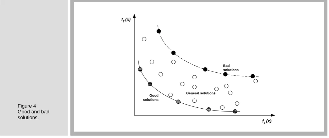
Apart from traditional learning from good solutions, COIN allows learning from below average solutions as well. Any coincidence found in a situation can be statistically described whether the situation is good or bad. Most traditional algorithms always discard the bad solutions without utilizing any information associated with them. In contrast, COIN learns from the coincidence found in the bad solutions and uses this information to avoid such situations to be recurrent; meanwhile, experiences from good coincidences are also used to construct better solutions in Figure 4. Consequently, the chances that the paths being parts of the bad solutions are always used in the new generations are lessened. This lowers the number of solutions to be considered and hence increases the convergence speed.

COIN uses a joint probability matrix (generator) to create the population. The generator is initialized so that it can generate a random tree with equal probability for any configuration. The population is evaluated in the same way as traditional evolutionary algorithms. However, COIN uses both good and bad solutions to update the generator. Initially, COIN searches from a fully connected tree and then incrementally strengthening or weakening the connections. As generations pass by, the probabilities of selecting certain paths are increased or decreased depending on the incidences found in the good or bad solutions. The algorithm of COIN can be stated as follows.

1. To initialize the joint probability matrix (generator); 2. To generate the population using the generator; 3. To evaluate the population;

4. To make diversity preservation;

5. To select the candidates according to two options: (a) good solution selection (select the solutions in the first rank of the current Pareto frontier), and (b) bad solution selection (select the solutions in the last rank of the current Pareto frontier);

General solutions Good

solutions

Bad solutions

f2 (x)

[image:13.595.36.562.371.592.2]

f1 (x) Figure 4

(14)

6. For each joint probability matrix H x x( ,_i _j), to adjust the generator according to the reward and punishment scheme as Eq.(10);

 

     

 

   

   

i j ij ij i j

i

ij i j

i

n n

j j

k

x t x t r t p t

n np

k

p t r t

n np

, , , ,

, ,

1 1

2

( 1) ( ) { ( 1) ( 1)}

( 1 )

{ ( 1) ( 1)}

( 1 )

where x_{i j}_, = the element ( , )i j of joint probability matrix H x( _i/x_j), k = the learning coefficient, r_{i j}_, = the number of coincidences ( ,x x_i _j) found in the good solutions, p_{i j}_,

= the number of coincidences ( ,x x_i _j)found in the bad solutions, t = generation number,

n = the size of the problem, and np_i = the number of the direct predecessors of task i; 7. To apply a strategy to maintain elitist solutions in the population, and then repeat step 2 until the terminating condition is met.

4.2 Numerical example

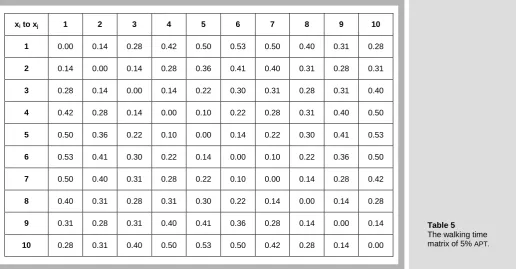
The 10-task problem of the single product with 10-minute cycle time originated by Miltenburg [3] is used to elaborate the algorithm of COIN. The manual task times are two time units for tasks 3, 4, 8, 9, 10, three time units for tasks 1, 7, and four time units for tasks 2, 5, 6. The precedence constraints are (3,1), (5,10), and (6,9). The fixed U-shaped layout of the side, front, and back is 2, 4, and 4 respectively. The walking time from one task to another task is five percent of average processing time. Since the total tasks time is 28, 0.05*(28 /10)  0.14. As a result, the walking time matrix of 5% APT for each element (x_{i j}_, ) is shown in Table 5. The task assignment rule is randomized. Learning probability ( )k and reward or punishment values are assumed to be 0.1. Population size is ten chromosomes and two generations are described step by step as follows.

4.2.1 Joint probability matrix initialization

The number of tasks to be considered is 10. Therefore, the dimension of From-To joint probability matrix H x x( ,_i _j) is the matrix 10x10. The value of each element (x_{i j}, ) in the matrix is the probability of selecting task j after task i. In order to incorporate some precedence relationship into the matrix, in each row the element which belongs to the direct predecessor of the task is set to 0 to prohibit producing such a task before its direct predecessor. For example, the direct predecessor of task 1 is task 3; hence,

1 3,

x = 0. Also, x_{1 1}, = 0, since it cannot move within itself. Initially, the value of the

xi to xj 1 2 3 4 5 6 7 8 9 10

1 0.00 0.14 0.28 0.42 0.50 0.53 0.50 0.40 0.31 0.28

2 0.14 0.00 0.14 0.28 0.36 0.41 0.40 0.31 0.28 0.31

3 0.28 0.14 0.00 0.14 0.22 0.30 0.31 0.28 0.31 0.40

4 0.42 0.28 0.14 0.00 0.10 0.22 0.28 0.31 0.40 0.50

5 0.50 0.36 0.22 0.10 0.00 0.14 0.22 0.30 0.41 0.53

6 0.53 0.41 0.30 0.22 0.14 0.00 0.10 0.22 0.36 0.50

7 0.50 0.40 0.31 0.28 0.22 0.10 0.00 0.14 0.28 0.42

8 0.40 0.31 0.28 0.31 0.30 0.22 0.14 0.00 0.14 0.28

9 0.31 0.28 0.31 0.40 0.41 0.36 0.28 0.14 0.00 0.14

[image:14.595.41.558.391.660.2]

10 0.28 0.31 0.40 0.50 0.53 0.50 0.42 0.28 0.14 0.00

Table 5 The walking time matrix of 5% APT.

(15)

67

remaining elements in the first row of the matrix are equal to

1

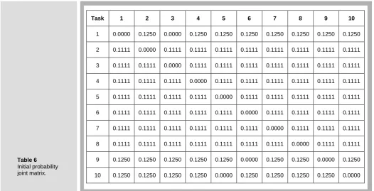
1/(n 1 np) 1/(10 1 1)   0.125. Continuing this computation for all the remaining tasks (rows), the initial joint probability matrix is shown in Table 6.

4.2.2 Population generation

The order representation scheme is used to create chromosomes. The task order list in a chromosome is created by moving forward from one task to another task. If more than one possible task can be selected, the probability of selecting any task will depend on its value on the joint probability matrix. In each generation, the first task (or the first order pair) is selected from the current elitist of the first Pareto-ranked chromosome(s). The same probability of selection will be randomized. For example, task 7 is randomly selected for the first position. After selecting the row of task 7, the set of eligible tasks comprises tasks 1 to 6 and 8 to 10. From row 7 of the joint probability matrix, a task is randomly selected according to its probability of selection

(p7,j0.1111, forj1,2,3,4,5,6,8,9,10). Supposing that task 6 is selected, the new set of

eligible tasks becomes tasks 1 to 5 and 8 to 10. This mechanism is continued as long as all positions in the task order list are filled in and the task order list of

L1={7,6,2,3,1,4,8,9,5,10} is obtained. As the population size is assumed to be 10, the nine remaining initial population consists of chromosomes L2={8,6,5,3,1,9,10,2,4,7},

L3={5,4,6,8,9,3,2,1,7,10}, L4={8,5,7,2,10,4,6,3,9,1}, L5={3,1,7,6,8,5,4,9,10,2}, L6={3,7,4,8,5,6,1,10,2,9},

L7={5,3,2,6,4,10,9,1,8,7}, L8={4,8,7,5,10,6,3,2,1,9}, L9={2,4,7,8,6,3,9,5,10,1}, and L10={2,3,6,8,4,1,7,5,10,9}.

4.2.3 Population evaluation

To find tentative tasks to be allocated on the U-line, all tasks have to be searched through the task order list in both forward and backward directions. The tentative task on forward or backward searching is found first. The task has its task time and walking time to the next task less than or equal to the remaining worker cycle time. If both forward and backward tentative tasks are found, either one is selected randomly. If any task from the task order list has not yet being allocated, a new workstation is opened. This procedure is repeated for the remaining task order list to obtain the number of workers (or workstations), walking time and worker load distribution for each of them. An example chromosome (L1) is shown in Table 7. The deviation of operation times of workers is calculated from Eq. (3) with Cjk= 7.28, 9.46, 6.46,and 6 28. respectively. Thus,

[image:15.595.36.563.87.356.2]

it is equal to 2.918 time units. The walking times of 0.14, 0.14, 0.14, 0.14, 0.10, 0.22, 0.10, 0.10, 0.14, 0.22, 0.14, and 0.14 are summed and the total walking time is equal to 1.72 time units. Having obtained feasible worker allocations three objectives have to be evaluated for each chromosome. Table 8 indicates that all chromosomes give the

Table 6 Initial probability joint matrix.

Task 1 2 3 4 5 6 7 8 9 10

1 0.0000 0.1250 0.0000 0.1250 0.1250 0.1250 0.1250 0.1250 0.1250 0.1250

2 0.1111 0.0000 0.1111 0.1111 0.1111 0.1111 0.1111 0.1111 0.1111 0.1111

3 0.1111 0.1111 0.0000 0.1111 0.1111 0.1111 0.1111 0.1111 0.1111 0.1111

4 0.1111 0.1111 0.1111 0.0000 0.1111 0.1111 0.1111 0.1111 0.1111 0.1111

5 0.1111 0.1111 0.1111 0.1111 0.0000 0.1111 0.1111 0.1111 0.1111 0.1111

6 0.1111 0.1111 0.1111 0.1111 0.1111 0.0000 0.1111 0.1111 0.1111 0.1111

7 0.1111 0.1111 0.1111 0.1111 0.1111 0.1111 0.0000 0.1111 0.1111 0.1111

8 0.1111 0.1111 0.1111 0.1111 0.1111 0.1111 0.1111 0.0000 0.1111 0.1111

9 0.1250 0.1250 0.1250 0.1250 0.1250 0.0000 0.1250 0.1250 0.0000 0.1250

(16)

same number of workstations; therefore, all of them are eligible for Pareto ranking based on Deviation of Operation times of Workers (DOW) and Walking Time (WT) objectives. The Pareto ranking technique proposed by Goldberg [32] is used to classify the population into non-dominated frontiers with a dummy fitness value that lower value is better. They are assigned to each chromosome in Figure 5.

Chromosome Number

Number of

workers DOW WT

Pareto

Frontier Crowding Distance

L5 4 2.8608 1.7373 1 Infinite

L1 4 2.9179 1.7197 1 Infinite

L10 4 2.8608 1.7783 2 Infinite

L2* 4 3.1136 1.7197 2 Infinite

L3* 4 3.1136 1.7197 2 Infinite

L8 4 2.9605 1.7960 3 Infinite

L7 4 3.1297 1.8773 4 Infinite

L4** 4 3.6619 1.9593 5 Infinite

L9** 4 3.6619 1.9593 5 Infinite

L6 4 4.0981 2.2400 6 Infinite

Table 8

Objective functions of each chromosome from the first

generation.

Dev iation of Operation times of Workers (seconds)

W a lk in g T im e ( s e c o n d s ) 4.25 4.00 3.75 3.50 3.25 3.00 2.3 2.2 2.1 2.0 1.9 1.8 1.7

Scatterplot of Pareto frontier

L6 Frontier#6 L4,L9 Frontier#5 L7 Frontier#4 L5 #1 L1 #1 L8 #3 L10 #2 L2,L3

#2 _{Figure 5}

[image:16.595.34.559.116.795.2]

Pareto frontier of each chromosome.

Table 7

An example of worker allocation in a single U-line.

Worker or Workstatio n Task considered Front graph Task considered Back graph

Task assignment on a U-line

(3) Total (1) + (2) Cycle time (time unit) (4) WT to Origin (time unit) (5) Given cycle time Idle time (time unit) (5)-(3)-(4) Task (1) WT (time unit) (2) Task time (time unit) 1 1 7 6 - 10 - 10 7 6 - 0.14 3 4 3 4.14 [7.14] - 0.14 10 7 2.72 2 2 2 2 3 1 - 10 - 10 - 10 2 3 1 - 0.14 0.10 4 2 3 4 2.14 [6.14] 3.10 [9.24] - 0.14 0.22

10 6

3.72 0.54 3 3 3 4 8 9 - 10 - 10 - 10 4 8 9 - 0.10 0.14 2 2 2 2 2.10 [4.10] 2.14 [6.24] - 0.10 0.22

10 8

(17)

69

4.2.4 Diversity preservation

COIN employs a crowding distance approach [32] to generate a diversified population uniformly spread over the Pareto frontier and avoids a genetic drift phenomenon (a few clusters of populations being formed in the solution space). The salient characteristic of this approach is that there is no need to define any parameter in calculating a measure of population density around a solution. The crowding distances computed for all solutions are infinite since at least two solutions are found for each frontier. Although both objectives of the chromosome L2 are the same as L3, and L4 are the same as L9, task sequence of each chromosome is different.

4.2.5 Solution selection

Having defined the Pareto frontier, the good solution is the chromosome located on the first Pareto frontier (dummy fitness = 1) and there is only one chromosome by the multiplication of reward value and population sizes, i.e. 0.1*10 = 1 solution. However, there are two solutions (L1and L5) in the first rank. One of both is randomized, i.e. L5 = {3,1,7,6,8,5,4,9,10,2}. In contrast, the bad solution is one located on the last Pareto frontier (dummy fitness = 6) and there is only one chromosome by the multiplication of punishment value and population sizes, i.e. 0.1*10 = 1, L6={3,7,4,8,5,6,1,10,2,9}.

4.2.6 Joint probability matrix adjustment

The adjustment of the joint probability matrix is crucial to the performance of COIN. Reward will be given to xi, j if the order pair (i, j) is in the good solution to increase the

chance of selection in the next round. For example, the first order pair (3,1) is the good solution of the chromosome L5 = {3,1,7,6,8,5,4,9,10,2}. Assumed that k=0.1 ; therefore, the value of xi, j where i=3 and j=1 is increased by k/(n-1-np3)=0.1/(10-1-0)=0.0111 The

updated value of xi, j of the order pair (3,1) becomes 0.1111+0.0111=0.1222 The values of the other order pairs located in the same row of the order pair (3,1) is reduced by k/(n-1-np3)

2

=0.1/(10-1-0)2=0.1/81=0.0012For example, the value xi, j where i=3 and j=1 is 0.1222-0.0012=0.121 For the other positions of j in the third row, each adjusted joint probability is 0.1111-0.0012=0.1099 Previously, the summation of probability of x3,j is equal to one. Continuing this procedure to all order pairs located in the good solution; the revised joint probability matrix is obtained in Table 9.

On the contrary, if the order pair (i, j) is in the bad solution, xi, j will be penalized to

reduce the chance of selection in the next round. For example, the first order pair (3,7) is in the bad solution of the chromosome L6={3,7,4,8,5,6,1,10,2,9}. Assuming thatk = 0.1;hence, the value of xi, j where i = 3 and j7 is decreased by k/(n-1-np3) =

0.1/(10-1-0) = 0.0111 The updated value of xi, j of the order pair (3,7), which is later

adjusted from Table 9 becomes 0.1099 – 0.0111 = 0.0988. The values of the other

order pairs located in the same row of the order pair (3,7) is increased by k/(n-1-np3)

2

=0.1/(10-1-0)2=0.1/81=0.0012 For example, the value xi, j where i=3 and j=7 is 0.0988+0.0012=0.1000. For the position of j=1 in the 3rd row, the adjusted joint probability is 0.1210+0.0012=0.1222. For the other positions of j in the third row,

Task 1 2 3 4 5 6 7 8 9 10

1 0.0000 0.1238 0.0000 0.1238 0.1238 0.1238 0.1349 0.1238 0.1238 0.1238

2 0.1111 0.0000 0.1111 0.1111 0.1111 0.1111 0.1111 0.1111 0.1111 0.1111

3 0.1210 0.1099 0.0000 0.1099 0.1099 0.1099 0.1099 0.1099 0.1099 0.1099

4 0.1099 0.1099 0.1099 0.0000 0.1099 0.1099 0.1099 0.1099 0.1210 0.1099

5 0.1099 0.1099 0.1099 0.1210 0.0000 0.1099 0.1099 0.1099 0.1099 0.1099

6 0.1099 0.1099 0.1099 0.1099 0.1099 0.0000 0.1099 0.1210 0.1099 0.1099

7 0.1099 0.1099 0.1099 0.1099 0.1099 0.1210 0.0000 0.1099 0.1099 0.1099

8 0.1099 0.1099 0.1099 0.1099 0.1210 0.1099 0.1099 0.0000 0.1099 0.1099

9 0.1238 0.1238 0.1238 0.1238 0.1238 0.0000 0.1238 0.1238 0.0000 0.1349

[image:17.595.39.560.475.655.2]

10 0.1238 0.1349 0.1238 0.1238 0.0000 0.1238 0.1238 0.1238 0.1238 0.0000 Table 9

(18)

each adjusted joint probability is 0.1099+0.0012=0.1111. Continuing this procedure to all order pairs located in the bad solution, the revised joint probability matrix is obtained in Table 10.

4.2.7 Elitism

To keep the best solutions found and to survive in the next generation, COIN uses an external list with the same size as the population size to store elitist solutions. All non-dominated solutions created in the previous population are combined with the current elitist solutions. Goldberg’s Pareto ranking technique is used to classify the combined population into several dominated frontiers. Only the solutions in the first non-dominated frontier are filled in the new elitist list. If the number of solutions in the first non-dominated frontier is less than or equal to the size of the elitist list, the new elitist list will contain all solutions of the first non-dominated frontier. Otherwise, tournament selection for Pareto domination [37] is exercised. Two solutions from the first non-dominated solutions are randomly selected and then the solution with larger crowding distance measure and not being selected before is added to the new elitist list. This approach not only ensures that all solutions in the elitist list are non-dominated solutions but also promoting diversity of the solutions. According to our example, the first-ranked elitist list from the first generation is L1={7,6,2,3,1,4,8,9,5,10} and

L5={3,1,7,6,8,5,4,9,10,2}. From Table 11, the task order list of the population size is

L11={7,6,2,3,1,4,8,9,5,10}, L12={8,2,7,5,10,4,3,6,1,9}, L13={8,4,7,2,5,6,3,9,1,10}, L14={3,5,7,4,2,10,1,6,8,9},

L15={4,3,5,7,1,10,6,9,2,8}, L16={5,4,3,2,10,7,6,9,1,8}, L17={8,3,2,1,5,4,7,10,6,9}, L18={6,5,4,2,9,7,8,10,3,1},

L19={7,5,8,3,6,10,9,1,2,4}, and L20={2,5,3,1,8,6,9,10,4,7}. The solutions in the current first non-dominated frontier is L11={7,6,2,3,1,4,8,9,5,10}, L13={8,4,7,2,5,6,3,9,1,10}, L15={4,3,5,7,1,10,6,9,2,8} and L20={2,5,3,1,8,6,9,10,4,7}. When the number of the combined solutions is less than the size of the elitist list, both solutions are added to the new elitist. Hence, five good solutions of current elitist list are L1 or L11={7,6,2,3,1,4,8,9,5,10}, L5={3,1,7,6,8,5,4,9,10,2},

[image:18.595.38.491.88.268.2]

L13={8,4,7,2,5,6,3,9,1,10}, L15={4,3,5,7,1,10,6,9,2,8} and L20={2,5,3,1,8,6,9,10,4,7}.

Table 10 Revised joint probability matrix (bad solution).

Task 1 2 3 4 5 6 7 8 9 10

1 0.0000 0.1250 0.0000 0.1250 0.1250 0.1250 0.1361 0.1250 0.1250 0.1139

2 0.1123 0.0000 0.1123 0.1123 0.1123 0.1123 0.1123 0.1123 0.1012 0.1123

3 0.1222 0.1111 0.0000 0.1111 0.1111 0.1111 0.1000 0.1111 0.1111 0.1111

4 0.1111 0.1111 0.1111 0.0000 0.1111 0.1111 0.1111 0.1000 0.1222 0.1111

5 0.1111 0.1111 0.1111 0.1222 0.0000 0.1000 0.1111 0.1111 0.1111 0.1111

6 0.1000 0.1111 0.1111 0.1111 0.1111 0.0000 0.1111 0.1222 0.1111 0.1111

7 0.1111 0.1111 0.1111 0.1000 0.1111 0.1222 0.0000 0.1111 0.1111 0.1111

8 0.1111 0.1111 0.1111 0.1111 0.1111 0.1111 0.1111 0.0000 0.1111 0.1111

9 0.1238 0.1238 0.1238 0.1238 0.1238 0.0000 0.1238 0.1238 0.0000 0.1349

(19)

71

4.2.8 Worker allocation

Finally, the results of 10-task worker allocation of a chromosome L1 or L11 in a single U-shaped assembly line are exemplified in Table 12 and Figure 6 and 7. Previously, its detailed calculation is clearly described in Table 7.

Task T (s.)

Worker 1:

7 6

3

3.14 7.28 10

Task Worker 4:

10 5

4 10

T (s.) 7.14

Task Worker 2:

1 3

9.2410 T (s.)

2

4

6.14

Task Worker 3:

9 8

2 4.24 10

T (s.)

4

4.10

4.14 6.24

9.46

2.10 6.246.46 4.14 6.146.28

Figure 7

Work load routines, showing allocation of four workers: solid line = manual time; wavy line = walking time; dashed line = idle time.

Chromosome Worker Manual time

Travel distance

time

Idle time

Allocated tasks (tk)

1 or 11 1 7 0.14 2.72 7 (3), 6 (4)

2 9 0.24 0.54 2 (4), 3 (2), 1 (3)

3 6 0.24 3.54 4 (2), 8 (2), 9 (2)

[image:19.595.41.561.43.236.2]

4 6 0.14 3.72 5 (4), 10 (2)

Table 12 Final exemplified results of Miltenburg’s 10-task worker allocation problem for a chromosome L1 or

L11.

Table 11

Objective functions of each chromosome from the second generation.

Chromosome Number

Number of

workers DOW WT

Pareto Frontier

Crowding Distance

L15 4 2.8338 1.8193 1 Infinite

L13 4 2.9090 1.7373 1 2.0000

L11* 4 2.9179 1.7197 1 Infinite

L20* 4 2.9179 1.7197 1 Infinite

L18 4 3.6878 1.9366 2 Infinite

L16** 4 4.0792 1.9593 3 Infinite

L17** 4 4.0792 1.9593 3 Infinite

L12*** 4 4.0853 1.9593 4 Infinite

L14*** 4 4.0853 1.9593 4 Infinite

L19*** 4 4.0853 1.9593 4 Infinite

In

Out

7

6

2

3

1

4

8

9

5

10 W1

W2

W3

W4

Figure 6

Final exemplified 10-task worker allocation results of a

chromosome L1 or L11

[image:19.595.39.561.317.799.2]

(20)

V. Experimental Results

5.1 Multi-objective solutions

In order to demonstrate the effectiveness of the proposed approach, computational results with multiple objectives are obtained on a set of single U-shaped assembly line worker allocation problems, which have 7 to 297 tasks set. From the previous results of convergence to the Pareto-optimal set, spread and ratio of non-dominated solution, and CPU time, COIN seems to perform better than well-known NSGA-II for most problem sets [26]. The multi-objective solution in this study is solved with hierarchical procedure. First, the objective function of a number of workers is minimized. Secondly, only a minimum number of workers are selected to further evaluate a pair of minimum DOW and WT objective values as the Pareto-optimum frontier. In this paper, the multi-objective coincidence algorithm is encoded and programmed by using MATLAB R2008a on an AMD AthlonTM 64 Processor 3500+ 2.21 GHz PC with 960 MB DDR-SDRAM., and the set of test problems are run at the 30 generations that are enough for attaining the major and minor aims in the paper.

5.2 A number of workers

In this section, a variety of proposed average processing time percentages is tested in every problem. The computational results of a number of workers at the symmetrical and rectangular layouts are shown in Table 13(a) and 13(b), respectively. A number of tasks that are representative in each problem are shown in the first column. The second column displays the summation of processing times. The cycle time is determined from test-bed problems [3],[7],[13],[26] in the third column. The theoretical number of workers in the fourth column is calculated with the second column divided by the third column. However, no paper displays the minimum number of workers for 7-task to 297-task U-shaped worker allocation problems with mathematical optimization techniques. Thus, the straight-line ULINO for the line balancing problem of type I [7] is benchmarked as the lower bound on quantity of workers in the fifth column. The values of a number of workers in various %APT display from column six to column twenty-one in every problem. The results show that the greater the walking time or %APT is, the larger the number of workers are. An example is shown in Figure 7.

From the experimental results of symmetrical and rectangular U-shaped layouts in Table 14, increasing only one worker in the first objective is sensitive to determining the walking time at only five percent of average processing time (or 0.14 to 65.61 seconds) in most problems. The 11-task problem is at the ten %APT (or 0.42 seconds.); the 19-task problem is at the 20 %APT (or 4.08 s.); and the 45-task problem is at the 15 %APT (or 1.84 seconds). It gives a conclusion that a decision to change a little walking time significantly effects the supplement of a larger number of workers in a single U-line. For every problem, the fixed average process time percentage shown in the second and third columns is representative to initial walking time that makes a number of workers different from the straight-line layout that is not taking walking time into account. The differences of a number of workers between both layouts for all problems are shown in the fourth column. A number of workers at the symmetrical U-line are the same as a number of workers at the rectangular U-U-line throughout a range of percentage for 7-task and 10-task problems due to their identical layouts at 1:3:3 and 2:4:4, respectively. From 11-task to 297-task problems, the first different values of number of workers between symmetrical and rectangular layouts are shown as each of %APT. However, from Table 13(a) and 13(b) they are different only one worker and for the rest of the first %APT of every problem a number of workers are mostly the same between symmetrical and rectangular U-line.