Power quality in microgrids

(1)

Power Quality in Microgrids

Thesis submitted in accordance with the requirements of the University of Liverpool for the degree of Doctor in Philosophy

by

Tomas Hornik

(2)

Abstract

Rapidly increasing energy demand from the industrial and commercial sector, especially in the current climate of high oil prices, steadily reducing energy sources and at the same time increased concerns about environmental changes, have caused fast development of Distributed Power Generation Systems (DPGS) based on renewable energy. A recent concept is to group DPGS and the associated loads to a common local area forming a small power system called a microgrid. This small autonomous system formed by DPGS can oer increased reliability and eciency of future power system networks. Furthermore, the improvement of the control capabilities and operational features of microgrids brings environmental and economic benets. The introduction of microgrids improves power quality, reduces transmission line congestion, decreases emission and energy losses, and eectively facilitates the utilisation of renewable energy resources.

As a consequence of the fast expanding DPGS based on renewable energy sources, Transmission System Operators (TSO) have issued strict interconnection requirements (grid code compliance), e.g., on power quality control, reactive power control, fault ride-through etc. Among these dierent requirements issued by the grid operators, power quality have recently gained a lot of attention due to excessive non-linear and unbalanced loads over-stressing the power systems and causing system failure. As nonlinear and/or unbalanced loads can represent a high proportion of the total load in small-scale systems, the problem with power quality is a particular concern in microgrids.

In this work, dierent control strategies are proposed and implemented for the grid and microgrid connected voltage-source inverters (VSI), based on H∞ and repetitive control techniques. The repetitive control, which is regarded as a simple learning con-trol method, oers very good performance for voltage and current tracking as it can deal with a very large number of harmonics simultaneously. This leads to a very low Total Harmonic Distortion (THD) of the output voltage and/or the current even in the presence of nonlinear loads and/or grid distortions.

(3)

controller can cope with grid frequency variations in the grid-connected mode. This mechanism allows the controller to maintain very good tracking performance over a wide range of grid frequencies.

Then, a H∞ repetitive control strategy for the inverter current is proposed and validated with experiments. As a result, the power quality and tracking performance are considerably improved. In order to demonstrate the improvements, the proposed controller is compared with the traditional resonant (PR), proportional-integral (PI) and predictive deadbeat (DB) controllers.

Finally, the advantages of the proposed voltage and current controllers based on H∞ and repetitive control techniques are put together for consideration in microgrid applications and experimentally tested. The proposed cascaded current-voltage control strategy is not a simple combination of the two control strategies, but a complete re-design after realising that the inverter LCL lter can be split into two separate parts for the design of the controllers. As a consequence, the cascaded controller is able to maintain low THD in both the microgrid voltage and the current owing into/from the grid at the same time. It also enables seamless transfer of the operation mode from standalone to grid-connected or vice versa. It turns out that the voltage controller can be reduced to a proportional gain cascaded with the internal model (in a re-arranged form), which can be easily implemented in real applications.

(4)

Acknowledgement

I would like to thank my supervisor Professor Qing-Chang Zhong for his encouragement, guidance and great support during the course of my PhD study. He was always ready to discuss the details of this work and share his expertise in control theory and power electronics, which has made this project enjoyable.

I would also like to thank my wife Pavla for her support and encouragement through-out my PhD.

Moreover, I would like to acknowledge the nancial support from the EPSRC UK (under the DTA scheme), and the departmental Research Support Budget.

(5)

List of Figures

2.1 Example of the microgrid structure with power electronics interfaced DPGS 7

2.2 General structure of the DPGS with full-scale power converters . . . 9

2.3 The block diagram of the conventional three-phase PLL system imple-mented indq synchronous reference frame . . . 13

2.4 The block diagram of a current-controlled VSI in the synchronously ro-tating reference frame (dq) . . . 14

2.5 The block diagram of a current-controlled VSI in the stationary reference frame (αβ) . . . 15

2.6 The block diagram of a current-controlled VSI in the natural frame (abc) 16 2.7 The standard H∞ optimal control problem . . . 19

2.8 The block diagram of an internal model . . . 20

2.9 The block diagram of the H∞ repetitive voltage control scheme . . . 21

2.10 Formulation of theH∞control problem . . . 22

3.1 Experimental setup . . . 24

3.2 Power electronics inverter board . . . 26

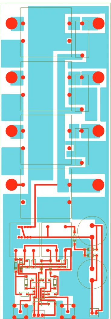
3.3 PCB 1 layout: three-phase LC lter and neutral point measurements . . 28

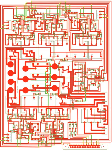
3.4 PCB 2 layout: three-phase voltage and current measurements . . . 29

4.1 The block diagram of a voltage-controlled VSI with the H∞ repetitive voltage controller in the natural frame . . . 31

4.2 The block diagram of the H∞ repetitive voltage control scheme . . . 32

4.3 Single phase representation of the plant P . . . 32

4.4 Bode plots of the discretised internal model . . . 35

4.6 Bode plots of the original and reduced controllers . . . 39

4.7 Stand-alone mode with a resistive load: (a) local load voltage uA, its reference voltageuref and voltage tracking erroreu, (b) local load current iA and (c) local load voltage uA and currentiA spectra . . . 40

(10)

4.9 Stand-alone mode with an unbalanced load: (a) local load voltages at the PCC and local load currents and (b) local load voltage uA and current

iA spectra . . . 42

4.10 Grid-connected mode without local load: (a) local load voltage uA, its referenceuref and voltage tracking error eu, (b) grid output currentiA, its referenceiref and current tracking errorei and (c) local load voltage uA and grid currentiA spectra . . . 43

4.11 Grid-connected mode with a resistive local load:(a) local load voltageuA, its reference uref and voltage tracking error eu, (b) grid output current iA, its reference iref and current tracking error ei and (c) local load voltageuA and grid currentiA spectra . . . 44

4.12 Grid-connected mode with a non-linear local load: (a) local load voltage uA, its reference uref and voltage tracking erroreu, (b) grid output cur-rentiA, its referenceiref and current tracking error ei and (c) local load voltageuA and grid currentiA spectra . . . 45

4.13 Grid-connected mode with an unbalanced local load: (a) local load volt-ages, (b) inverter (upper) and grid output currents (lower) and (c) local load voltageuA and grid current iA spectra . . . 47

4.14 Transient response in the grid-connected mode without local load to1A step change inId∗: (a) local load voltageuA, its referenceuref and voltage tracking erroreu, (b) grid output currentiA, its referenceiref and current tracking errorei . . . 48

4.17 Responses to grid frequency variations (f = 50.00Hz) with (a) and with-out (b) the frequency adaptive mechanism (local load voltage uA, its reference voltageuref and tracking error eu) . . . 49

4.15 Responses to grid frequency variations with (left) and without (right) the frequency adaptive mechanism: (a) f = 49.85Hz, (b) f = 49.90Hz and (c) f = 49.95Hz (local load voltage uA, its reference voltage uref and tracking erroreu) . . . 50

4.16 Responses to grid frequency variations with (left) and without (right) the frequency adaptive mechanism: (a) f = 50.05Hz, (b) f = 50.10Hz and (c) f = 50.15Hz (local load voltage uA, its reference voltage uref and tracking erroreu) . . . 51

5.1 The block diagram of a current-controlled VSI with the H∞ repetitive current controller in the natural frame . . . 54

5.2 The block diagram of the H∞ repetitive current control scheme . . . 55

5.3 Single phase representation of the plant P . . . 55

5.5 Bode plots of the original and reduced controllers . . . 60

(11)

6.1 The block diagram of a current-controlled VSI in the natural frame (abc) 63 6.2 Single phase representation of the plant . . . 63 6.3 Root locus of the closed loop system . . . 64 6.4 Bode plots of the open-loop system for dierent Ki . . . 65

6.5 Single phase representation used to derive DB controller equation . . . . 66 6.6 Dierent current control strategies comparison in the grid-connected mode

without local load: (a) H∞ repetitive controller, (b) PR controller, (c) PI controller and (d) DB controller . . . 69 6.7 Current spectra comparison in the grid-connected mode without local

load: (a) H∞ repetitive controller, (b) PR controller, (c) PI controller and (d) DB controller . . . 69 6.8 Dierent current control strategies comparison in the grid-connected mode

with a resistive local load: (a)H∞repetitive controller, (b) PR controller, (c) PI controller and (d) DB controller . . . 70 6.9 Current spectra comparison in the grid-connected mode with a resistive

local load: (a) H∞ repetitive controller, (b) PR controller, (c) PI con-troller and (d) DB concon-troller . . . 70 6.10 Dierent current control strategies comparison in the grid-connected mode

with an unbalanced local load: (a)H∞repetitive controller, (b) PR con-troller, (c) PI controller and (d) DB controller . . . 72 6.11 Current spectra comparison in the grid-connected mode with an

unbal-anced local load: (a) H∞ repetitive controller, (b) PR controller, (c) PI controller and (d) DB controller . . . 72 6.12 Dierent current control strategies comparison in the grid-connected mode

with a non-linear local load: (a) H∞ repetitive controller, (b) PR con-troller, (c) PI controller and (d) DB controller . . . 73 6.13 Current spectra comparison in the grid-connected mode with a non-linear

local load: (a) H∞ repetitive controller, (b) PR controller, (c) PI con-troller and (d) DB concon-troller . . . 73 6.14 Transient responses comparison in the grid-connected mode without local

load: (a) H∞ repetitive controller, (b) PR controller, (c) PI controller and (d) DB controller . . . 74

7.1 The block diagram of a VSI with the cascaded H∞ repetitive current-voltage controller in the natural frame(abc) . . . 77 7.2 The block diagram of the H∞ repetitive voltage control scheme . . . 78 7.3 Single-phase representation of the control plantPufor the voltage controller 79

(12)

7.8 Bode plots of the original and reduced controllers . . . 84 7.9 Stand-alone mode with a resistive load: (a) local load voltage uA, its

reference voltageuref and voltage tracking erroreu, (b) local load current

iA and (c) local load voltage uA and currentiA spectra . . . 85

7.10 Stand-alone mode with a non-linear load: (a) local load voltage uA, its

reference voltageuref and voltage tracking erroreu, (b) local load current

iA and (c) local load voltage uA and currentiA spectra . . . 87

7.11 Stand-alone mode with an unbalanced load: (a) local load voltage at the PCC and local load currents, (b) local load voltage uA and current iA

spectra . . . 88 7.12 Grid-connected mode without local load: (a) local load voltage uA, its

referenceuref and voltage tracking error eu, (b) grid output currentiA,

its referenceiref and current tracking errorei and (c) local load voltage

uA and grid currentiA spectra . . . 89

7.13 Grid-connected mode with a resistive local load: (a) local load voltageuA,

its reference uref and voltage tracking error eu, (b) grid output current

iA, its reference iref and current tracking error ei and (c) local load

voltageuA and grid currentiA spectra . . . 91

7.14 Grid-connected mode with a non-linear local load: (a) local load voltage uA, its reference uref and voltage tracking erroreu, (b) grid output

cur-rentiA, its referenceiref and current tracking error ei and (c) local load

voltageuA and grid currentiA spectra . . . 92

7.15 Grid-connected mode with an unbalanced local load: (a) local load volt-ages, (b) inverter (upper) and grid output currents (lower) and (c) local load voltageuA and grid current iA spectra . . . 93

7.16 Transient response in the grid-connected mode without local load to1A step change inId∗: (a) local load voltageuA, its referenceuref and voltage

tracking erroreu, (b) grid output currentiA, its referenceiref and current

tracking errorei . . . 94

7.17 Transient response of the inverter, while transferred from stand-alone to the grid-connected mode and vice versa: (a) grid output current iA, its

reference iref and current tracking error ei, and (b) local load voltage

uA, its reference uref and voltage tracking error eu . . . 95

7.18 Detail of the response to transfer from stand-alone to grid-connected mode at timet= 1sec: (a) grid output current iA, its reference iref and

current tracking errorei, and (b) local load voltageuA, its referenceuref

(13)

7.19 Detail of the step response to change in the grid output current I_d∗ ref-erence from 0A to 1.5A at time t = 3sec: (a) grid output current iA,

its referenceiref and current tracking errorei, and (b) local load voltage

uA, its reference uref and voltage tracking error eu . . . 97

7.20 Detail of the response to transfer from grid-connected to stand-alone mode at timet = 7.08sec: (a) grid output current iA, its reference iref

and current tracking errorei, and (b) local load voltageuA, its reference

(14)

List of Tables

2.1 Maximum current harmonic distortion . . . 8

4.1 Parameters of the plant . . . 33

6.1 Current spectra comparison in the grid-connected mode without local load . . . 68 6.2 Current spectra comparison in the grid-connected mode with a resistive

local load . . . 71 6.3 Current spectra comparison in the grid-connected mode with an

unbal-anced local load . . . 71 6.4 Current spectra comparison in the grid-connected mode with a non-linear

local load . . . 74

7.1 Current and voltage spectra comparison in the stand-alone mode with a resistive local load . . . 86 7.2 Current and voltage spectra comparison in the stand-alone mode with a

non-linear local load . . . 86 7.3 Current and voltage spectra comparison in the stand-alone mode with

an unbalanced local load . . . 87 7.4 Current and voltage spectra comparison in the grid-connected mode

with-out local load . . . 90 7.5 Current and voltage spectra comparison in the grid-connected mode with

a resistive local load . . . 90 7.6 Current and voltage spectra comparison in the grid-connected mode with

a non-linear local load . . . 90 7.7 Current and voltage spectra comparison in the grid-connected mode with

(15)

Chapter 1

Introduction

1.1 Motivation

The DPGS are usually active at the distribution level and provide an alternative to the traditional large centralised facilities, such as coal, nuclear or gas powered power plants, where currently most of the electricity is generated. DPGS are usually small-scale, typ-ically in the range of 3 kW to 10MW. Rapidly increasing energy consumption on one side and steadily reducing energy sources and climate change on the other side, lead to the need for DPGS based on renewable energy sources, mainly from wind and solar energy. The electricity generated from these sources is not in the form needed by the public grid and often needs to be processed so that it can be connected to the grid. Fol-lowing technological developments, especially higher power ratings, lower losses, more reliable performance and lower price, modern power electronics are becoming more and more attractive and are used as an interface between DPGS and the utility grid, as they match the characteristics of the DPGS and the requirements of grid connections. For example wind turbines using power converters can operate with a variable speed and are designed to achieve maximum aerodynamic eciency over the wide range of wind speed. Since the wind turbine operates at a variable rotational speed, the electrical frequency of the generator varies and must therefore be decoupled from the frequency of the grid. The electrical system of the variable-speed turbine is more complex, how-ever using power electronics increases its energy capture, improves power quality and reduces the mechanical stress on the wind turbine. In general, power electronics im-prove the performance of the DPGS and provide the DPGS with power system control capabilities, improve power quality and their eect on power system stability.

(16)

integration into the power system. For example, the increasing size of the wind farms resulted in an interconnection request at the transmission level. As a consequence, grid operators requirements are becoming stricter and there is strong emphasis on the ability of the DPGS to have power plant characteristics. This means that DPGS have to be able to behave as an active controllable component in the power system and meet very high technical standards, such as voltage and frequency control, active and reactive power control, quick responses during faults in the utility grid, harmonics minimisa-tion etc. DPGS based on the renewable energy sources are changing from being minor energy sources to acting as important power sources with power plant characteristics in the energy systems. The control strategies applied to DPGS have become of high interest and need to be further investigated and developed [1, 2, 3].

A more recent concept is to group a cluster of loads and parallel DPGS in a com-mon local area to form a microgrid. Being a larger entity, a microgrid possesses a larger power capacity and more control exibilities to full system-reliability and power-quality requirements, in addition to all inherited advantages of a single DPGS. Moreover, improving the control capabilities and operational features of microgrids brings environmental and economic benets. The introduction of microgrids leads to improved power quality, reduces transmission lines congestion, decreases emission and energy losses, and eectively facilitates the utilisation of renewable energy resources [4, 5, 6, 7, 8, 9, 10, 11, 12, 13].

In this work, dierent control strategies based on the H∞ and repetitive control techniques are proposed for grid and microgrid connected VSI. The main objective of the proposed controllers is to inject a clean sinusoidal voltage and current to the power system, even in the presence of non-linear loads or grid voltage distortions. The repeti-tive control technique, based on the well-known internal model principle, is adopted as it can deal with a very large number of harmonics simultaneously and oers excellent performance for voltage and current tracking and harmonics reduction.

1.2 Outline of the thesis

The thesis is organised as follows. In Chapter 2, the development and importance of microgrids are discussed and the general structure of DPGS based on renewable energy sources is described. The main control tasks of the grid-side converter are summarised and primary grid operators requirements are shortly introduced. In addition, the dier-ent control schemes and classical control methods implemdier-ented to the grid-side converter are presented. Finally, the former work on H∞ repetitive voltage controller design is briey described.

(17)

In Chapter 4, a voltage controller based on H∞ and repetitive control techniques proposed in literature is further developed and experimentally tested. Attention is paid to improving power quality and tracking performance, and considerably reducing the complexity of the controller design. Moreover, a frequency adaptive mechanism is proposed so that the controller can cope with grid frequency variations in the grid-connected mode.

In Chapter 5, the voltage control strategy proposed in Chapter 4 is replaced with a current control strategy and the H∞ repetitive current controller is developed and experimentally tested. As a result, the power quality and tracking performance are considerably improved.

In order to demonstrate the improvements, the proposed H∞ repetitive current controller is compared, in Chapter 6, with the traditional PR, PI and DB controllers with the main focus on harmonics distortion and tracking performance.

The advantages of voltage and current controllers based on the H∞ and repetitive control techniques are brought forward for consideration in microgrid applications and experimentally tested in Chapter 7. We show that, the proposed control strategy is able to maintain low THD in both the microgrid voltage and the current owing into/from the grid at the same time.

Finally, the main conclusions of the thesis are summarised and possible future work is proposed in Chapter 8.

1.3 Major contributions

1.3.1 H∞ repetitive voltage controller

The voltage controller based onH∞ and repetitive control techniques proposed in [14] is further developed and experimentally tested. We have strived to improve power quality and tracking performance, while considerably reducing the complexity of the controller design. We propose a frequency adaptive mechanism, so that the controller can cope with grid frequency variations, while operating in the grid-connected mode. This mechanism allows the controller to maintain very good tracking performance over a wide range of grid frequencies. Another major improvement in this work with respect to [14] is that, following extensive simulations and real-time experiments, the model of the plant has been reduced to single-input-single-output (SISO) repetitive control design. As a consequence, the design becomes much simpler than the one proposed in [14] and the stability evaluation is easier.

1.3.2 H∞ repetitive current controller

(18)

a result, the power quality and tracking performance are considerably improved. In addition, the proposed controller is compared with the traditional PR, PI and DB con-trollers with the main focus on harmonics distortion and tracking performance.

1.3.3 H∞ repetitive cascaded current-voltage controller

The advantages of voltage and current controllers, proposed in this work, are put to-gether for consideration in microgrid applications and experimentally tested. The strat-egy adopts a voltage repetitive controller cascaded with a current repetitive controller and is not a simple combination of the two control strategies, but a complete re-design after realising that the inverter LCL lter can be split into two separate parts for the design of the controllers. A strategy simultaneously reduces the THD in both the mi-crogrid voltage and the current owing to/from the grid at the same time. What is novel and inventive is that low THD in both the current and voltage can be achieved simultaneously. The known strategies can achieve only one or the other. It is also worth mentioning that the current controller is in the outer loop and the voltage controller is in the inner loop. Normally, when a current controller and a voltage controller are cascaded, the current controller is in the inner loop and the voltage controller is in the outer loop. Moreover, the strategy allows a smooth seamless transition of operation mode between the standalone mode and the grid-connected mode. The strategy can be used for single-phase systems or three-phase systems.

1.4 List of publications

Research monograph

1. Q.-C. Zhong and T. Hornik. Control of Power Inverters for Distributed Generation and Renewable Energy, Wiley-IEEE Press, to appear in 2011.

Journal papers

1. T. Hornik and Q.-C. Zhong. H∞repetitive voltage control of grid-connected inverters with frequency adaptive mechanism. IET Power Electronics, accepted for publication, July 2010.

2. T. Hornik and Q. -C. Zhong. A current control strategy for grid-connected voltage-source inverters based onH∞ and repetitive control, under review. 3. Q. -C. Zhong and T. Hornik. CascadedH∞ repetitive current-voltage control of

(19)

Conference papers

1. T. Hornik and Q.-C. Zhong. Control of grid-connected DC-AC converters in distributed generation: Experimental comparison of dierent schemes. In proceedings of the6th International Conference-Workshop Compatibility and Power Electronics (CPE 2009), pages 271 278, May 2009.

2. T. Hornik and Q.-C. Zhong. H∞repetitive current controller for grid-connected inverters. In proceedings of the35th _{Annual Conference of IEEE Industrial}

Electronics (IECON 2009), pages 554 559, November 2009.

3. T. Hornik and Q. -C. Zhong. Voltage control of grid-connected inverters based onH∞ and repetitive control. In proceedings of the 8th World Congress on Intelligent control and Automation (WCICA 2010), July 2010, Shortlisted for: Best student paper and Best application paper.

(20)

Chapter 2

Background

In this chapter, the development and importance of the microgrids are discussed. The general structure of the DPGS based on renewable energy sources are described. The main control tasks of the grid-side converter are summarised and primary grid operators requirements are shortly introduced. In addition, the dierent control schemes and classical control methods implemented to the grid-side converter are presented. The developments of theH∞and repetitive control techniques are also introduced. Finally, the former work of the voltage controller design is briey presented.

2.1 Microgrids

Microgrids are emerging as a consequence of rapidly growing distributed power gen-eration systems. Compared to a single DPGS, the microgrid has more capacity and control exibilities to full system reliability and power quality requirements. In a typical microgrid, the micro-sources may be rotating generators or Distributed Energy Resources (DER) interfaced by power electronic inverters. The installed DERs may be biomass, fuel cells, geothermal, solar, wind, steam or gas turbines. The microgrid also oers opportunities for optimising DPGS through the combined heat and power (CHP) generation, which is currently the most important means of improving energy eciency. The connected loads may be critical or non-critical. Critical loads require a reliable source of energy and good power quality [11, 15]. An example of the microgrid structure with power electronics interfaced DPGS is shown in Figure 2.1. The microgrid is connected to the utility system through a circuit breaker, also called Static Transfer Switch (STS) at the Point of Common Coupling (PCC). The circuit breaker ensures that the microgrid can be disconnected from the main grid promptly in the event of a utility interruption. As shown in Figure 2.1, two DPGS are employed in the micro-grid. Each DPGS system comprises an energy source, an energy storage system, and a grid-interfacing inverter.

(21)

Energy

source storage Energy Inverter

Critical load 1

Energy

source storage Energy Inverter

Critical load 2

Non-critical load Microgrid

DPGS 1 DPGS 2

Circuit breaker PCC

[image:21.595.125.515.70.320.2]

Line Line

Figure 2.1: Example of the microgrid structure with power electronics interfaced DPGS

to supply at least a part of the load after being disconnected from the distribution system and to remain operational as a standalone (islanded) system [5, 8, 10]. Traditionally, the inverters used in microgrids behave as current sources when they are connected to the grid and as voltage sources when they work autonomously [16]. This involves the change of the controller when the operational mode changes from standalone to grid-connected or vice versa.

As nonlinear and/or unbalanced loads can represent a high proportion of the total load in small-scale systems, the problem with power quality is a particular concern in microgrids [17]. Moreover, unbalanced utility grid voltages and utility voltage sags, which are two most common utility voltage quality problems can aect microgrid power quality [18, 19]. The microgrid control and operational features should be able to cope with an unbalanced utility grid voltages and voltage sags within the range given by the nature and waveform quality requirements of the local loads and/or microgrids. When critical loads are connected to a microgrid, severe unbalanced voltages are not generally acceptable and the microgrid should be disconnected from the utility grid. However, when the voltage unbalance is not so serious or the local load is not very sensitive to it, the microgrid can remain connected.

2.2 Requirements of Transmission System Operators

(22)

on renewable systems, the system operators have issued more strict interconnection requirements, e.g., on power quality control, reactive power control, fault ride-through etc. [1, 2, 20]. The interconnection requirements dier signicantly between countries. This depends on the properties of each power system as well as the level of the DPGS penetration (mainly wind power systems). In other words, countries with a very low DPGS penetration do not necessarily need to accept strict requirements as countries that have substantial proportion of the DPGS connected to the power system. In general the requirements are intended to ensure that the DPGS have the control and dynamic properties needed for operation of the power system with respect to both short-term and long-short-term security of supply, voltage quality and power system stability. For example in Denmark, the country with the largest penetration of wind power in the power system, the wind farm has to be able to contribute to the control task on the same level as conventional power plants, constrained only by the limitation of existing wind conditions [1].

Odd harmonics Maximum harmonics current distortion

<11th _<_4%

11th₋₁₅th _<_2%

17th−21st <1.5% 23rd−33rd <0.6%

>33rd <0.3%

Table 2.1: Maximum current harmonic distortion

A common requirement in all standards is the power quality of the distributed power. The power quality assessment, is mainly based on harmonics. Harmonics are a phenomenon associated with the distortion of the voltage and current waveforms (periodic voltage or current disturbances with frequencies multiple of the fundamental frequency). Harmonics, induced by non-linear loads, increase the total Root-Mean-Square (RMS) value of line currents, and thus may cause additional power losses on grid lines and abnormal heating of transformers, induction motors, power-factor correction capacitors etc.. Depending on the harmonic order, these may cause excessive stress and damage of various kinds to the dierent types of electrical equipment. Furthermore, an important property of harmonics is that they tend to be cumulative on a power system, i.e. the contributions of the various harmonics sources add up to some degree. Consequently, harmonics currents have a negative impact on power systems [21, 22].

THD is used in electrical engineering to evaluate the disturbance extent and can be calculated as

T HD=

s

∞

P

I2

n n=2

I1 (2.1)

where, I1 is the fundamental current magnitude in RMS and In is nth harmonic

(23)

current harmonics [23, 24]. For both wind turbine and photovoltaic connected to the utility grid, the maximum limit for the total harmonic distortion of the output voltage

isT HD= 5% (120V-69kV).

2.3 Introduction to DPGS structure and control

A general structure of a distributed power generation system depends on the input power nature (wind, sun, etc.). Dierent hardware congurations are possible [21]. Figure 2.2 shows general structure of the DPGS using back-to-back full-scale power electronic converters. This bidirectional power converter, consists of two conventional pulse-width modulated (PWM) converters, and is nowadays becoming more and more attractive in DPGS integration [1]. The input-side converter, controlled by input-side controller, normally ensures that the maximum power is extracted from the input power source and transmits the information about any available power to the grid-side controller. The main objective of the grid-side converter is the interaction with the utility grid. The grid-side controller usually has the following tasks: power quality control, active and reactive power control and grid synchronisation [25]. In following subsections, the tasks of the grid-side controller are discussed in more details.

Input-side Converter

Grid-side Converter

Output Filter

Transformer

Input-side controller Grid-side controller

Power quality Power flow Grid synchronization DC-link voltage

Maximum power extraction Input–side protection

Figure 2.2: General structure of the DPGS with full-scale power converters

2.3.1 Power quality control

(24)

To compensate low-order harmonics and meet grid operators requirements, dier-ent control and harmonics compensation strategy approaches are employed. Usually the current controller is responsible for power quality issues and should have a very good harmonic rejection. Dierent types of controllers (for example PI controllers, PR controllers or non-linear controllers such as hysteresis or dead-beat) implemented in dierent reference frames provide the system with a dierent quality of the harmonics rejection [27, 28].

The switching frequency of PWM switching converter is usually a few kilohertz and high-order frequency harmonics are small in magnitude and can be removed by a l-ter. The lter is connected in parallel as an interface between inverter and utility grid [29, 30, 31, 32, 33, 34]. Short lter topologies description follows.

L Filter

This topology consists of an inductive lter connected in series with the inverter. Although being the topology with the fewer number of components, the system dy-namics is poor due to the voltage drop across the inductor causing long time responses. Moreover, in order to attenuate the inverter harmonics, the inverter switching frequency must be high [34, 35].

LC Filter

This topology consists of a capacitor and an inductor. With higher values of capaci-tance, the inductance can be reduced, leading to reduction of losses and cost. However, very high capacitance values are not recommended, since problems may arise with in-rush currents, high capacitance current at the fundamental frequency and dependence of the lter on grid impedance for overall harmonic attenuation. Moreover, using line-side capacitors for harmonics reduction, form together with lter inductance and/or line inductance an LC resonant circuit. A lightly damped LC resonance may cause serious oscillation or over-voltages that may destroy the switching devices and other components [22, 35, 36].

LCL Filter

The LCL lter has a better attenuation than an LC lter (lower ripple current stress) and small a dependence on the grid parameters, with smaller component values, which is a signicant advantage in high-power applications. Moreover, LCL lters pro-vide inductive output at the grid interconnection point to prevent inrush current [33, 35].

(25)

The simplicity and high reliability of this solution is therefore the reason that it is widely used in industry. However, the additional resistor losses are a substantial disadvantage. Therefore, nowadays, there is a tendency to replace passive damping by active damping [38, 39, 40, 41, 42].

2.3.2 Power ow control

One task of the grid-side controller is the power ow control. The power ow control means to regulate the active and reactive power exchange between DPGS and the utility grid.

The active power control is associated with frequency control. The frequency of a power system is proportional to the rotating speed of the synchronous generators operating in the system. Increasing the electrical load in the system tends to slow down the generators and reduce the frequency. The task of frequency control of the system is to increase or reduce the generated power so as to keep the generators operating within the specied frequency range. However, renewable resources can only produce when the source is available. In order to be able to increase the power output for frequency control, DPGS may have to operate at a lower power level than the available power, which means low utilisation of the energy resources. The situation may be improved by use of an energy storage technology, such as batteries or fuel cells [21].

While the active power is associated with frequency control, the reactive power is linked to voltage control. Conventional reactive power concepts are associated with the oscillation of energy stored in capacitive and inductive components in a power system. Reactive power is produced in capacitive components and consumed in inductive com-ponents. The current associated with the reactive power ow causes system voltage drop and also power losses. Furthermore, large reactive currents owing in a power sys-tem may cause voltage instability in the network due to the associated voltage drops in the transmission lines [21]. Following operators requirements, DPGS have to contribute to voltage regulation in the power systems. The requirements either refer to a certain voltage range that has to be maintained at the point of connection of the DPGS, or to a certain reactive power compensation that has to be provided [1].

As the real and reactive power control is important, the DPGS equipped with power electronics converters take advantage that the control of the reactive power can be decoupled from active power control. For this purpose, the synchronously rotating reference (dq) frame is commonly used, as the scheme has the particular advantage of independent control of the real and reactive current components.

2.3.3 Grid synchronisation

(26)

run over short grid disturbances (fault ride-through). This means maintaining running system, when short voltage or frequency variation occurs in the grid network. The phase angle used in DPGS generating the grid current reference, should be clean signal, synchronised with the grid voltage. Hence, it is important for DPGS to have a fast and accurate detection of the positive-sequence component of the utility voltage [43], in order to keep the generation up according to grid connection requirements. A short overview of dierent synchronisation methods follows.

Zero crossing method

One of the simplest methods for obtaining the phase information is to detect the zero crossing of the utility voltages. However, the zero crossing points can only be detected at every half cycle of the utility voltage frequency. Thus the dynamic performance of this technique is quite low [27, 28].

αβ anddq lter algorithms

The phase angle of the utility grid voltage can also simply be obtained by ltering the input signals. Depending on the reference frame, where the ltering is applied, two structures can be implemented: ltering inαβ stationary reference frame and ltering indqsynchronous rotating reference frame. Improved performance over the zero cross-ing method is reported, but still, the ltercross-ing technique encounters diculty to extract the phase angle when grid variations or faults occur in the utility network [27].

PLL

Nowadays, the phase-locked loop (PLL) technique is usually used to extract the phase angle of the grid voltage [27]. The conventional PLL system implemented within the dq synchronous reference frame [44], shown in Figure 2.3, uses a PI controller to track the phase angle of the grid voltages and the lock is realised by setting the refer-ence of the d−axis voltage to zero. Under ideal grid conditions, this PLL structure performs satisfactory. However, when the utility grid is unbalanced, improvements to the conventional three phases PLL are necessary.

(27)

abc

PI controller

θ

uα uβ

ua ub uc

-

αβ

αβ dq

ud*

ud

θ 1

s

uq

Figure 2.3: The block diagram of the conventional three-phase PLL system implemented indq synchronous reference frame

signal at the fundamental frequency, but also other sequence components at higher frequencies.

2.4 Control schemes for grid-side converters

Currently, most grid-side converters adopt the VSI topology with a current controller to regulate the current injected into the grid [49, 50, 51, 52]. Current controlled inverters have the advantages of the high accuracy control of an instantaneous current, a peak current protection, an overload rejection and very good dynamics [53]. The basic control structure of the grid-side controllers is a fast internal current loop, which regulates the grid current, and an external voltage loop, which controls the dc-link voltage [27]. The current loop is responsible for power quality issues and the dc-link voltage controller is designed for balancing the power ow in the system. Such control structures can be implemented into dierent reference frames. A basic division of the control schemes with respect to the dierent reference frames follows.

2.4.1 Synchronously rotating reference frame control

Synchronous reference frame control, also called dq, uses abc → dq transformation module to transform the control variables from their natural frame abc to a dq frame, which synchronously rotates with the frequency of the grid voltage. This transformation is commonly used in three-phase systems, where it is known as the Park transformation.

The grid voltage in natural frame can be represented as

vabc=Vm



 

cosθg

cos(θg−2₃π)

cos(θg+2₃π)





(28)

abc dq + - + -

Id Iq

θ

Id*

Iq*

Ud

Uq

uga ugc

PLL ugb PWM modulation Ud Uq + + + + dq abc DC power source Inverter bridge LC filter Transformer Current controller ia ib ic

abc dq θ Current controller -ωL ωL Iq

Id + +

Figure 2.4: The block diagram of a current-controlled VSI in the synchronously rotating reference frame (dq)

where Vm is the peak value of the grid voltage and θg is the phase angle. If the grid

voltage is balanced, the (2.2) can be expressed in stationary(αβ) frame as

vαβ =Tαβ∗vabc, (2.3)

wherevαβ =

h

vα vβ

iT

and transform matrix

Tαβ =

2 3

1 −1

2 − 1 2 0 − √ 3 2 √ 3 2 ! . (2.4)

Equation (2.3) can be further be expressed in synchronous(dq) reference frame as

vdq =Tdq∗vαβ, (2.5)

wherevdq =

h

vd vq

iT

and transform matrix

Tdq =

2 3

cosθg −sinθg

sinθg cosθg

!

. (2.6)

As a consequence, the control variables are DC signals, and controlling and/or ltering such values is easier. Thedq control algorithm is normally associated with PI control.

(29)

(oth-abc

αβ

+ -

Iα Iβ

Id*

Iq* uga ugc

PLL

ugb

PWM modulation

αβ

dq

DC power

source Inverter bridge filterLC

Transformer

ia ib ic

abc

αβ

θ uβ uα

Iβ* Iα* Current controller

Current controller

Figure 2.5: The block diagram of a current-controlled VSI in the stationary reference frame (αβ)

erwise, a controller can be introduced to regulate the DC-link voltage and to generate I_d∗ accordingly).

2.4.2 Stationary reference frame control

In the stationary reference frame control, also calledαβ, the grid voltages and currents are transformed into the reference frame using abc → αβ transformation (2.3). The control variables are sinusoidal and the diculty comes in designing a regulator with the correct gain against frequency characteristic to regulate the fundamental frequency and reject higher harmonic disturbances. PI regulators with their pole (innite gain) at zero-frequency are not best suited to this task and it is unable to eliminate steady state error [27]. A proportional resonant (PR) controller is usually used. The block diagram of a current-controlled VSI in the stationary reference frame (αβ) is shown in Figure 2.5. It has a current loop including a PR controller so that the current injected into the grid could track the reference currentsi∗_α and i∗_β, which are generated from the d, q-current reference I_d∗ and I_q∗ using a dq → αβ transformation. A PLL is used to provide the phase information of the grid voltage, which is needed to generate i∗_α and i∗_β. The real power and reactive power exchanged with the grid are determined by I_d∗ andI_q∗.

2.4.3 Natural frame control

(30)

DC power source

Inverter bridge

LC filter

Transformer

PWM modulation

Id*

Iq*

iref

abc dq θ

PLL

ugb

uga ugc

ia ib ic

- +

- + Current controller

Current controller

[image:30.595.128.508.74.230.2]

Current controller

Figure 2.6: The block diagram of a current-controlled VSI in the natural frame (abc)

be also implemented to theabcframe [25].

In a situation of an isolated neutral transformer (4 −Y), used as DPGS grid inter-face, only two of the grid currents can be independently controlled, the third one being the negative sum of the other two according to Kirchho's law. Hence, the implemen-tation of two controllers only is necessary.

All controllers used in this work are implemented in the abc frame with a Y −Y step-up transformer being used as the interface between utility grid and experimental setup. The system is implemented with a neutral point controller proposed in [54]. An individual controller is used for each phase (see Chapter 3 for more details).

2.5 Classical control methods

As stated in the previous Section 2.4, most of the grid-connected inverters currently adopt the VSI topology, with a current controller to regulate the current injected into the grid by using schemes such as proportional-integral (PI) controllers in the synchronously rotating reference frame (dq), proportional-resonant (PR) controllers in the stationary reference frame (αβ), predictive deadbeat controllers or hysteresis controllers in the natural (abc) frame [25, 27, 37, 49, 50, 51, 52, 55]. The short overview of the most popular control methods implemented in dierent frames follows.

2.5.1 Proportional-integral control

A PI [25, 56, 57] controller is normally associated with the synchronous reference frame control ordq control. The transfer function of the PI controller is given by

CP I(s) =Kp+

Ki

s , (2.7)

whereKp and Ki are proportional and integral gains respectively.

(31)

solution for regulating sinusoidal current in balanced three-phase systems, however is not good at correcting unbalanced disturbance currents which are a common feature of distribution systems [14]. Moreover, compensation capability of the low-order harmon-ics, using PI controllers, are poor. The PI controller in a synchronous frame is more complex with respect to a PR controller in the stationary frame, as it is requires two coordinate transformations with knowledge of the synchronous frequency. In addition the synchronousdq transformation can't be applied to single-phase systems.

To improve the performance of a PI controller in this structure, cross-coupling terms (±ωL) and/or feed-forward grid voltage (Ud and Uq), shown in Figure 2.4, can be

used [25, 27]. The feed-forward grid voltage is used in order to improve dynamics of the controller during grid voltage uctuation. Every deviation of the grid voltage amplitude is reected into thed- andq-axis component of the voltage, leading to a fast response of the control system [56]. In addition, the scheme has the particular advantage of independent control of the real and reactive current components, which translates directly to real and reactive power ow control. This is advantageous for application, where the grid supply currents can be directly regulated in the synchronous frame and transferred back into the natural frame to provide references for PWM modulation [37]. For more details, including PI controller design, see Chapter 6.

2.5.2 Proportional-resonant control

A PR [58, 59, 60, 61, 62] controller is usually used in a stationary reference frame control αβ, however it can easily be implemented in an abcframe. Such a controller has got a high gain around resonant frequency and thus is capable of eliminating a steady state error, when control variables are sinusoidal [25, 27, 61]. The transfer function of a proportional resonant controller is given by

CP R(s) =Kp+Ki

s

s2₊_ω2 (2.8)

where ω is resonant frequency. In this structure a low order harmonics compensator can be easily implemented to improve the performance of the current controller without inuencing its behaviour [25]. The transfer function of the harmonics compensator is given by

CHC(s) =

X

h=3,5,7,..

Kih

s

s2_{+ (}_ωh₎2 (2.9)

(32)

2.5.3 Deadbeat control

Deadbeat (DB) predictive controllers [63, 64, 65, 66, 67, 68, 69, 70, 71, 72, 73, 74, 75] are widely employed for sinusoidal current regulation of dierent applications due to its high dynamic response. This controller theoretically has a very high bandwidth, and hence, tracking of sinusoidal signals is very good. The principle of the DB controller is to calculate the derivative of the controlled variable in order to predict the eect of the control action. Deadbeat predictive control is widely used for current error compensation and oers high performance for current-controlled VSIs. However, it is quite complicated and sensitive to system parameters [55, 56]. For more details, including DB controller design, see Chapter 6.

2.5.4 Hysteresis control

Hysteresis control [76, 77, 78] is simple and brings fast responses. Normally, the output of the hysteresis comparator is the state of the switches in the power inverter, hence three hysteresis controllers are required (one for each leg of the inverter) in the case of a three phase inverter. Three-phase output currents of the inverter are detected and compared with the corresponding phase current references individually. The switch-ing signals are produced directly when the error exceeds an assigned tolerance band. Hysteresis control is insensitive to system parameters and is extremely simple for imple-mentation. Moreover, due to the closed-loop PWM, hysteresis control oers an inherent current protection and usually an outstanding dynamic response. However, since the three-phase currents are independently controlled with a control delay, which virtually eliminates the ability to generate zero voltage vectors, the output current ripples may be quite large and the THD of the output currents could be unacceptably high for power grids. Moreover, the inverter switching frequency depends largely on the load parameters and varies with the ac voltage. Due to the inherent randomness, caused by the limit cycle, the output lter design is dicult.

A number of proposals have been put forward to overcome variable switching fre-quency. Depending on the method used, the complexity of the controller can be in-creased considerably. Although the constant switching frequency scheme is more com-plex, it guarantees very fast response together with limited tracking error. The constant frequency hysteresis controls are well suited for high performance high-speed applica-tions [25, 27, 55, 76, 77, 79].

2.5.5 Multiloop control

(33)

with the outer loop ensuring steady-state reference tracking performance and the inner loop providing fast dynamic compensation for system disturbances (including sudden reference or load changes) and improving stability [80].

For example in [37] a strategy is proposed to control the grid output current of an inverter connected to the grid through a LCL lter. The PI controller is used to regulate the grid current, together with a simple inner capacitor current regulating loop to stabilise the system.

In stand-alone systems, a multiloop voltage controller with a capacitor current feed-back as inner loop can eliminate the output LC lter resonant peak to increase stability in load disturbance and enhance dynamic performance [81, 82, 83].

G

C

u

z

w

[image:33.595.234.412.250.381.2]

y

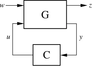
Figure 2.7: The standard H∞optimal control problem

2.6 H

∞

theory and repetitive control

In this section theH∞ and repetitive control techniques are briey introduced and the former work of the voltage controller design is presented.

2.6.1 Introduction to H∞ control theory

(34)

Riccati equations [84]. The mathematical symbol H∞ comes from the name of the mathematical space over which the optimisation takes place (hardy space). TheH∞is the space of matrix-valued functions that are analytic and bounded in the open right-half of the complex plane.

The standard H∞ optimal control problem is shown in Figure 2.7, where w rep-resents an external disturbance, y is the measurement available to the controller, u is the output from the controller, and z is an error signal that it is desired to keep small. The transfer function G represents not only the conventional plant to be con-trolled, but also any weighting function included to specify the desired performance. The H∞ optimal control problem is then to design a stabilising controller C, so as to minimise the closed loop transfer function from w to z,Tzw, in the H∞ norm, where

kTzwk∞=sup

ω∈<

¯

σ(Tzw(jω))[85].

Developed late in the last century, robust control has been widely used in industrial plants. TheH∞control method have been applied to power electronics, for example to boost converters [86], grid-connected inverters [14, 13], or a Dynamic Voltage Restorer (DVR) system [84].

W(s) e-τds

+ +

e

p

Figure 2.8: The block diagram of an internal model

2.6.2 Repetitive control

(35)

inverters [89, 90, 91, 92, 93, 94, 95, 96, 97], grid-connected inverters [14, 13, 98] and active lters [99, 100, 101].

2.6.3 H∞ repetitive voltage controller proposed in [14]

In this section the previous work from literature, which is the base of this work, is briey presented. For more details, please refer to [14].

The block diagram of the H∞ repetitive control scheme is shown in Figure 2.9, whereP is the transfer function of the plant,C is the transfer function of the stabilis-ing compensator and M is the transfer function of the internal model. The stabilising compensator C, designed by solving a weighted sensitivity H∞ problem, assures the exponential stability of the entire system, which implies that the tracking error e be-tween the voltage reference and the inverter output voltage will converge to a small steady-state error. The internal model M is a local positive feedback of a delay line cascaded with a low-pass lterW(s).

Vref

plant

stabilizing

compensator

u

e

Vg

i

d

ic

s d

e

s

W

(

)

−τ

+

internal model +

w

p

P

M

C

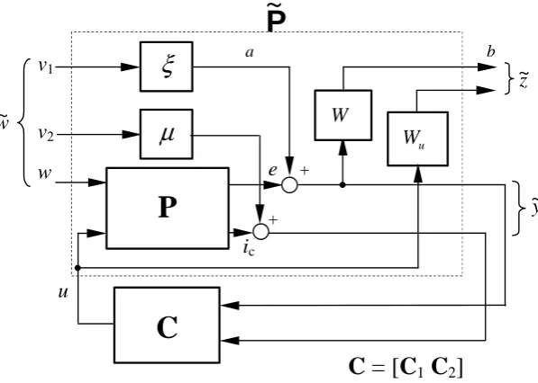
Figure 2.9: The block diagram of theH∞ repetitive voltage control scheme In order to guarantee the stability of the system, the H∞ control problem, as shown in Figure 2.10, is formulated to minimise the H∞ norm of the transfer func-tion Tz˜w˜ = Fl( ˜P , C) from w˜ = [v₁v₂w]T to z˜ = [ z₁ z₂ ]T, after opening the local positive feedback loop of the internal model and introducing weighting parameters ξ andµ. The closed-loop system is represented as

" ˜ z ˜ y

#

= ˜P

" ˜ w u

#

,

u=Cy,˜

(36)

P

C

u

e w

ic

W

+

µ

ξ

u W v1

v2

a b

P

~

z~

y

~

w~

[image:36.595.172.471.76.289.2]

C = [C

1

C

2

]

+

Figure 2.10: Formulation of the H∞control problem

However, in simulations and experiments, some practical problems were discovered. Some of these problems were already treated in [102], unfortunately the design becomes even more complex than the one presented in [14].

(37)

Chapter 3

Experimental setup

In order to carry out real-time experiments an experimental setup has been designed and built up. In this chapter, the experimental system design and development are briey described.

3.1 System structure

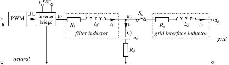
The experimental setup consists of an inverter board, a phase LC lter, a three-phase grid interface inductor, a three-three-phase local load, a board consisting of voltage and current transducers, a step-up transformer, a dSPACE DS1104 R&D controller board with ControlDesk software, and MATLAB Simulink/SimPower software package. The experimental setup and block diagram of the experimental setup are shown in Figures 3.1 (a) and (b) respectively.

The inverter board consists of two independent three-phase inverters and has the capability to generate PWM voltages from a constant 42V DC voltage source. The generated three-phase voltage is connected to the grid via a controlled circuit breaker and a step-up transformer. The grid voltage and the current injected into the grid are measured for control purposes. The sampling frequency of the controller is 5 kHz

and the PWM switching frequency is 12 kHz. A Yokogawa power analyser WT1600 is

used to measure the THD. Following sections consist of short descriptions of all major components of the experimental setup.

3.2 Software environment

(38)

(a) Experimental setup

Circuit breaker and grid interface

inductor Lg

Measure 2 Measure 1

PCB 2 PCB 1

Local load

DC power

source Inverter bridge filterLC

Transformer

dSpace 1104

da db dc if uf ig ug

[image:38.595.129.519.165.616.2]

(b) The block diagram of the experimental setup

(39)

ability test a variety of time-varying systems, including apart from other digital signal processing and controls.

SimPower Systems [104] extends the Simulink software with tools for modelling and simulating basic electrical circuits and detailed electrical power systems. These tools allow model the generation, transmission, distribution, and consumption of electrical power.

3.3 dSPACE Kit

The dSPACE Kit used in this work consists of three major components. These are DS1104 controller board [105, 106], CP1104 connector board and the ControlDesk soft-ware [107, 108].

DS1104 controller board is real-time hardware based on PC technology for controller development in various elds, such as drives, robotics, aerospace or automotive. The DS1104 controller board upgrades PC to a development system for rapid control proto-typing. This real time interface (RTI) provides MATLAB/Simulink with library blocks for graphical conguration of ADC, DAC, digital I/O lines, incremental encoders, PWM blocks etc.. Simulink models can be then easily congured and run by using these RTI blocks. This reduces the implementation time to a minimum.

CP1104 connector board is an I/O interface between the power electronics drives board and DS1104 controller board. CP1104 connector board is used to easily access I/O signals with BNC and Sub-D connectors.

Finally the ControlDesk is a test and experiment software for DS1104 controller de-velopment. The ControlDesk manages real-time and Simulink experiments. It performs all the necessary tasks in a single working environment. The ControlDesk can operate in two basic modes: the developer mode with the full functionality, and the operator mode. The control of Simulink simulations is integrated to validate controller models oine, switching into the dSPACE real-time and back again as required. The Con-trolDesk can use the same tool environment for virtual instrumentation, automation, and parameter set handling, without any modications at all.

3.4 Power electronics inverter board

(40)

before being fed to the drivers. The drive board consists of over-current protection for each inverter. Voltage measurement test points are provided to observe the inverter output voltages and current transducers are used to measure the output current of the inverters. The PWM/digital signals and other digital signals for the board are realised by the 37-pin DSUB connector.

Figure 3.2: Power electronics inverter board

3.5 Step-up transformer

The three-phase step-up transformer is used in this work to transform the low level voltages generated by the power electronics drives board to values necessary for utility grid connection. A transformer has been manufactured according to design requirements by the Majestic Transformer Company. Transformer specication: Three-phaseY −Y connection, primary voltage: 12VRM S (line to neutral) 50/60Hz, secondary voltage:

230VRM S (line to neutral), power rating: 400V A.

3.6 Filters, sensors and signal conditioning circuits

To build up an experimental setup, shown in Figure 3.1, two printed boards (PCB 1 and PCB 2) have been designed. PCB 1, shown in Figure 3.3, consists of a three-phase LC line lter (Lf and Cf), components to create neutral point and two independent

circuits to measure variables required for neutral point control. The three-phase LC line lter is provided to reduce higher-order harmonics generated by the power electronics inverter board. The neutral leg topology consists of two split capacitorsCN+and CN−

and inductor LN. The two variables to be measured which are required for neutral

point control are voltage shiftεof the neutral point and current through capacitors iC

(41)

PCB 2, shown in Figure 3.4, consists of a three-phase circuit breaker, grid inter-face inductorLg and two sets of three phase voltages and line currents measurements.

The rst set measures voltages and currents on the inverter-side of the circuit breaker including local load. The second set measures grid voltages and currents exchanged between grid and the experimental setup. The grid voltage measurements are necessary for synchronisation. Each of the measurement circuits consist of a LEM transducer and 2nd order low pass lters. The LV 25-P and LA 25-NP transducers are used to mea-sure voltages and currents respectively. Both transducer types have galvanic isolation between the primary circuit (high power) and the secondary circuit (electronic circuit). The analog output signal from each transducer (secondary circuit) is further processed through a 2nd order low pass lter, to eliminate ripples at switching frequency of the DC-AC converter. Since the total number of analog variables to be measured is higher with respect to availability of the input ADC channels on the dSPACE DS1104 Con-troller board, three four-channels analog multiplexers are introduced on PCB 2. The three-phase circuit breaker is realised by three independent relays controlled by signals from the dSPACE DS1104 Controller board.

(42)

[image:42.595.227.411.122.649.2]

(43)

R 2 C3 R 4 J 7 J 8 J 9 J 1 0 J 1 1 F 1 F 2 F 3 J 1 3 C5 R 3 C1 C4 R 1 C 7 C 9 C 1 0 R M 1 C3 4 C 8 R34 C27 C28 C29 R2 5 S O C K E T 4 M W C30 R1 0 R1 2 R 2 8 R30 S O C K E T 4 M N S O C K E T 4 M V S O C K E T 4 M P S O C K E T 4 M O S O C K E T 4 M M RM 5 1 0 6 1 M + _ 5 L A 2 5 N T RM 6 C 3 9 L M 3 5 8 A Q R M 1 2 C5 1 C 4 0 C3 1 C3 2 C3 5 C3 3 C3 6 C 3 7 C 3 8 R 1 3 R 1 4 R 1 5 R 1 6 R M 7 R M 8 10 6 1 M + _ 5 LA 25 NS 10 6 1 M + _ 5 LA 25 NU M _ + -H T +H T LV 25 V M _ + -H T +H T LV 25 T C 5 7 C 5 8 R M 1 1 C5 3 C5 4 C5 5 C5 6 C4 1 C4 2 M _ + -H T +H T LV 25 U C4 3 C4 4 C4 5 C4 6 C 4 7 C 4 8 C 4 9 C 5 0 L M 3 5 8 A R R 1 7 R 1 8 R 1 9 R 2 0 L M 3 5 8 A S R M 9 R M 1 0 C 5 9 C 6 0 M _ + -H T +H T LV 25 W R 2 2 R 2 3 R 2 4 R29 L M 3 5 8 A O 10 6 1

M + _

5 LA25NQ C15 C13 C12 R M 4 R M 3 R 8 R 7 R 6 R 5 C 2 0 C 1 9 C 1 8 C 1 7

M + _

-HT +HT LV25Q R2 6 S O C K E T 4 M U R M 2

M + _

-HT +HT

LV25P 10 6

1

M + _

5 LA25NP L M 3 5 8 A N C2 R V 7 ADG509D B N C 3 C 2 1 C 2 2 LM 35 8A P C 2 3 C 2 4 C 2 5 R9 R1 1 C 2 6 AD G5 09 B J 1 2 R V 9 R V 8 C5 2 R 2 1 B N C 4 ADG509E C 6 8 C14 C11 C 6 4 C 6 2 B N C 1 C16 1 0 6 1 M + _ 5 L A 2 5 N R RV6 T 1 SU B3 7 C 6 7 C 6 9 R V 1 0 C65 C 6 6 J 1 4 S O C K E T 4 M Q C6 3 C6 1 C6 S O C K E T 4 M S R E L B A R E L A Z R E L A Y S O C K E T 4 M R R M 1 R 2 C 1 0 R 1 C 9 C 2 C 8 ic 2 C 7 C 3 L M 3 5 8 A N C 5 C

4 C1

ia

1 va

[image:43.595.134.522.132.654.2]

1 R M 2 R 3 R 4 R 4 ib 2 -1 2 V R 3 R M 2 R M 1 R 2 C 1 0 R 1 C 9 C 1 C 2 C 8 C 6 C 7 C 3 L M 3 5 8 A N C 5 C 4 v a 2 ia 2 v c 1 v b 1 C6 G N D C 1 C 4 C 5 L M 3 5 8 A N C 3 C 7 C 6 C 8 C 2 C 9 R 1 C 1 0 R 2 R M 1 R M 2 R 3 R 4 C 8 C 2 C 9 R 1 C 6 v c 2 v b 2 C 1 C 4 C 5 L M 3 5 8 A N C 1 0 C3 LM 35 8A N C5 C4 C1 R 2 R M 1 R4 R3 RM 2 RM 1 R2 C1 0 R1 C9 C2 C8 + 1 2 V C7 R M 2 R 3 R 4 L M 3 5 8 A N C 5 C 7 C 3 C 4 C 1 C 3 C 7 C 6 C 8 C 2 C 9 R 1 C 1 0 R 2 R M 1 R M 2 R 3 R 4 ic 1 ib C 6 -1 2 V G N D + 1 2 V + 1 2 V -1 2 V G N D

Power quality in microgrids