Study of Flow Pattern in Jet Clarifier for Removal of Turbidity by Residence Time Distribution Approach

Article

Study of Flow Pattern in Jet Clarifier for Removal of

Turbidity by Residence Time Distribution Approach

Ploypailin Romphophak

_*

_{, Kritchart Wongwailikhit}

_{, Nattawin Chawaloesphonsiya}

_,

Pornsak Samornkraisorakit

_{, and Pisut Painmanakul}

1 Department of Environmental Engineering, Faculty of Engineering, Chulalongkorn University, Bangkok 10330, Thailand

2Metropolitan Waterworks Authority, Bangkok 10210, Thailand

3 Research Unit Control of Emerging Micropollutants in Environment, Chulalongkorn University, Bangkok 10330, Thailand

E-mail: a_{[email protected] (Corresponding author),} b_{[email protected]}

Abstract. This study aims to determine the performance of the jet clarifier for turbidity removal and its mechanisms for proposing the optimal operating conditions and design criteria. The experiment were performed continuously using a pilot scale jet clarifier with the volume of 243 L. Effects of liquid flow rates, types of liquid phase, and sludge blanket heights on turbidity removal efficiency were investigated. Moreover, the residence time distribution (RTD) study was carried outto investigate the flow pattern. The results indicated that the jet clarifier can effectively reduce the turbidity of the synthetic water with the efficiency of 80%under the optimal condition. The RTD results suggested that the flow pattern in the jet clarifier corresponded to the design as the plug flow and mixed flow conditions were found in the coagulation and the flocculation/sedimentation zones, respectively. The presence of the sludge blanket can reduce the bypass and recirculated flows. Besides, the increase of flow rate resulted in the increase recirculation in the tank. It can be suggested that the jet clarifier can be used for removing turbidity in the water treatment. The hydrodynamic in the reactor, which relates to flow pattern in the reactor, is one among the important factors in a jet clarifier.

Keywords: Jet clarifier, turbidity removal, residence time distribution (RTD).

ENGINEERING JOURNAL Volume 20 Issue 2 Received 21 September 2015

Accepted 19 November 2015 Published 18 May 2016

1.

Introduction

The jet clarifier is a type of solid contact clarifier considered as an effective and compact system for water treatment [1]. It can be implied as sludge recirculation units with a static mixer for destabilization. This system consists of two sections including mixing and settling zones. At the mixing zone, raw water is mixed with coagulants and injected through the centre of the reactor. Flocculation occurs as destabilized particles would aggregate into flocduring flowing upward. Flocs can be separated in a settling zoneand deposit forming a sludge blanket. Afterwards, sludge was separated from the clarified water in a settling zone where sludge is deposited and recirculated through the central zone by the induced zone. According from this process, the enrichment can induce the rapid flocculation and the formation of a dense precipitates. Moreover, the jet clarifier is also comprised of a sludge hopper in order to eliminate the excess sludge [1-3]. Consequently, hydrodynamical modelling of jet clarifier is highly important, at least from the following two perspectives: because of its influence on the performance of a given plant and because of its role in scaling-up from pilot tests.

Modern methods, residence time distribution (RTD) were developed and applied to predict hydrodynamic behaviors in reactor [4]. The measurement is obtained from tracer experiment that consists of an impulse response method. The injection of a tracer is conducted at the system inlet and a probe is introduced at the outlet to record the concentration-time relation [5]. The relationship can be used to construct the exit age distribution in reactor, which indicates the flow pattern in reactor. The different regions of a reactor can be modeled as that of mix flow or plug flow reactor having dead spaces with bypassing between zones [4]. The determination of RTD is frequently combined with the modelling of the system using one, two or three-parameter models, either based in mass balance or in statistical analysis [6, 7]. Therefore, RTD measurement can be an efficient tool for better understanding the hydrodynamic condition in the reactor. This information can be applied for designing reactor as well as scale-up, operation, and optimization [7, 8].

The objectives of this work were to determine the performance of jet clarifier for turbidity removal in the aspect of water treatment. Effects of flow rates, sludge blanket height, and water types were investigated. The flow behaviour in the reactor was also analysed by the RTD. The information obtained from this work could be utilized for designing the reactor design and suggesting the appropriate operation for a jet clarifier.

2.

Materials and Methods

2.1. Liquid Phases

The liquid phases were the synthetic raw water and the real surface raw water from Prapa canal along Samsen Water Treatment Plant. The synthetic water was prepared by mixing bentonite used as model colloidal particles with tap water. To simulate the real raw water, the initial turbidity was adjusted to 501 NTU, which equals the average raw water turbidity of the Samsen plant [9]. The stock synthetic raw water was stirred by an agitator to ensure that the bentonite particles were dispersed thoroughly.

2.2. Experiment Set-up

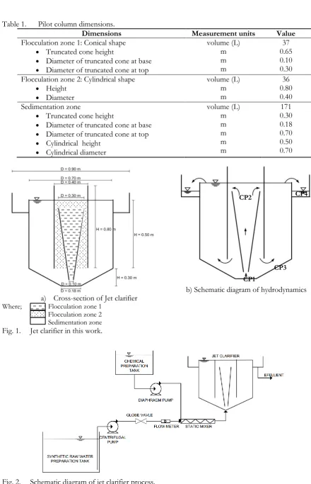
The reactor was made from an acrylic material with the dimension as presented in Table 1. Figure 1 shows a cross-section of the jet clarifier and a schematic diagram of hydrodynamics.

2.3. Experimental Procedures

The jet clarifier was operated continuously in both two parts of the experiments. The first part was to study the turbidity removal efficiency of the jet clarifier. Aluminum sulfate (Al2(SO4)3∙18H2O) was used as

Table 1. Pilot column dimensions.

Dimensions Measurement units Value

Flocculation zone 1: Conical shape

 Truncated cone height

 Diameter of truncated cone at base

 Diameter of truncated cone at top

volume (L) m m m

37 0.65 0.10 0.30 Flocculation zone 2: Cylindrical shape

 Height

 Diameter

volume (L) m m

36 0.80 0.40 Sedimentation zone

 Truncated cone height

 Diameter of truncated cone at base

 Diameter of truncated cone at top

 Cylindrical height

 Cylindrical diameter

volume (L) m m m m m

171 0.30 0.18 0.70 0.50 0.70

a) Cross-section of Jet clarifier Where; Flocculation zone 1

Flocculation zone 2 Sedimentation zone

b) Schematic diagram of hydrodynamics

Fig. 1. Jet clarifier in this work.

Fig. 2. Schematic diagram of jet clarifier process.

CP1 CP2

2.4. Operating Conditions of Jet Clarifier

The system can be divided into 2 parts including the rapid mixing by the static mixer and the slow mixing followed by the sedimentation in the jet clarifier. The retention time from each part at different flow rates is compared with those from the conventional processes for turbidity removal as shown in Table 2. The designed retention time of the jet clarifier was in the same range with the criteria. Note that G values in the static mixer and the jet clarifier were controlled by the liquid flow rates, while the gradient in the jar test were kept constant.

Table 2. Comparison of contact or retention time of the jet clarifier to the design criteria.

Category Flow rate _(L/hr) Coagulation _{time (s)} Flocculation _{time (min)} Sedimentation _{time (hr)} Reference

Design

criteria - 1 < t < 5 20 – 40 1 – 3 [1,10,11,12]

Jet clarifier

40 3.31 50 4.66

50 2.65 40 3.72

70 1.89 30 2.79

110 1.20 20 1.86

180 0.74 13.16 1.25

2.5. Analytical Methods

The turbidity and pH were measured by the turbidity meter (Lovibond, Germany) and the pH meter (Hach, USA), respectively. The standard methods 2540D and 2320B were applied for analysing suspended solid and alkalinity [13]. The turbidity removal efficiency was evaluated from Eq. (1).

 

i C f C i C % removal

Turbidity _

        (1)

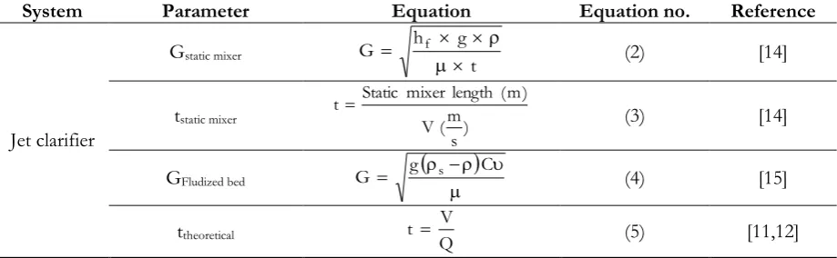
The considered parameters in this work can be calculated by Eq. (2) – (5) in Table 3.

Table 3. Parameters in jet clarifier experiments.

System Parameter Equation Equation no. Reference

Jet clarifier

Gstatic mixer

t g h G f     

 (2) [14]

tstatic mixer ₎

s m ( V ) m ( length mixer Static t 

(3) [14]

GFludized bed G  g





ttheoretical _Q

V

t  _{(5) [11,12]}

The residence time distribution (RTD) was conducted for analyzing the behavior of non-ideal reactors. Two single parameter flow model was used to characterize the RTD results. Although other analysis methods are available, the compartment model and the dispersion model were chosen due to their simplicity and applicability [16]. The method of moments and non-ideal device techniques were used to calculate the parameters from the experimental data, including mean residence time (tm), variance (2), exact

variance (2_{) and flow model parameter [17, 18]. The tracer (NaCl) pulse input data are presented using}

the exit-age distribution function E(t) which is defined as the fraction of material which has left the device between time t and t+dt. The function E(t) with the unit of min-1 _{can be expressed as}

dt = E(t) on; Distributi ime Resident T

0 (t)

) t ( C

C

where C(t) is the concentration of the tracer at time t. The mean residence time (tm) and variance (2) were

calculated by Eq. (7) and (8), respectively.

dt E t dt E E t

t

t

t







m

(

)

)

(

)

(

( (t)

0 m 2

2

 



 (8)

The exact variance (2_{) as in Eq. (9), which is the ratio of the variance to the square of the}

experimental mean residence time, is used to predict the dispersion number ( ). The is the dimensionless parameter that directly gives an indication of the flow regime. The value of one corresponds to the completely mixed, while the value of zero indicates the perfect plug-flow conditions.





2 m

2

2 _{1 e}

uL D 2 uL D 2 t                     (9)

where D = dispersion coefficient (m2_{/s), u = velocity gradient (m/s) and L = Flow distance (m).}

3.

Results and Discussions

3.1. Turbidity Removal by Jet Clarifier

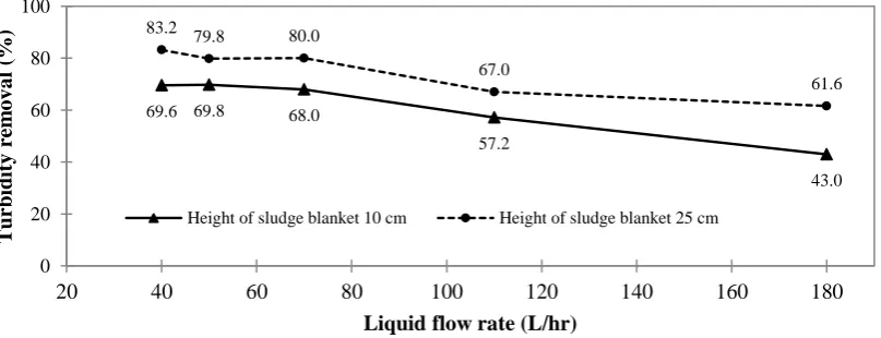
Effects of liquid flow rate and sludge blanket height on turbidity removal efficiency: Figure 3 illustrates the turbidity removal as a function of flow rates and sludge blanket heights. For the synthetic raw water, the efficiency was decreased when raising the flow rate. The highest efficiencies of 68% and 80% can be achieved at the flow rates of 40 – 70 L/hr for the blanket heights of 10 cm and 25 cm, respectively. Similar results were obtained from the actual raw water with the highest efficiency of 81% at 70 L/hr and 25 cm height; therefore, they are not shown here. Moreover, pH of the treated water was in the neutral range (7.0 – 7.5) [19]. In addition, the efficiency of this jet clarifier was similar to the approximately 80% of the Samsen Water Treatment Plant 1, which uses a jet pulsator and sedimentation in a conventional rectangular tank for 6 hours [20, 21].

Fig. 3. Comparison of turbidity removal efficiency as a function of liquid flow rates.

In summary, the liquid flow rates and the sludge blanket heights were key factors in the design and operation due to their effects on efficiency. The optimal condition in this work can be suggested at the sludge blanket height of 25 cm and the liquid flow rate of 70 L/hr (retention time of 197 minutes).Note that the lower efficiency of the jet clarifier compared to the jar test was a result of different operation modes, which are continuous and batch systems, respectively.

Effects of flow rate on the efficiency can be explained by the velocity gradient (G) and retention time (t). The lower flow rates of 40 L/hr and 50 L/hr gave insufficient G for slow mixing but provided large retention time. This allowed particles to separate from water by settling resulting in the good efficiency. On

69.6 69.8 _68.0

57.2

43.0

83.2 _{79.8 80.0}

67.0 61.6 0 20 40 60 80 100

20 40 60 80 100 120 140 160 180

T urbid it y re m o v a l (%)

Liquid flow rate (L/hr)

the contrary, the jet clarifier was ineffective in the turbidity removal at the flow rates higher than 70 L/hr due to its short retention time. Moreover, the height of the sludge blanket also affected the efficiency. As the cumulative sludge volume would be recirculated to the flocculation zone, it can increase the contact probability between particles and enhance the agglomeration of destabilized particles forming larger solid flocs [1, 11].

Effect of liquid flow rate on design parameters: Table 4 presents the parameters considered in this study at different operating conditions. The reasonable ranges of the liquid flow rates in this study suggested by the suitable G, t, and G∙t values in the design criteria were 50, 70, and 110 L/hr. These flow rateswere then applied to study the turbidity removal efficiency and effects of sludge blanket height.

Table 4. Operating conditions performed by various G, t and G∙t values.

Method Liquid flow _{rate (L/hr)} Mechanism _(sG _{-1) (s)} t (G∙t) sed a

(hr)

Jet b

(hr)

Design criteria*

- coagulation > 350 1 < t < 5 < 1700c

1-3 -

- flocculation < 5d _{1200-2400 10}4_-105

Pilot plant

40 _flocculation coagulation 243.76 _{0.562 3000} 3.31 807.68 ₁₆₈₆ 4.66 5.49

50 _flocculation coagulation 340.67 _{0.630 2400} 2.65 903.02 ₁₅₁₂ 3.72 4.39

70 _flocculation coagulation 564.32 _{0.743 1800} 1.89 1068.47 _1337.40 2.79 3.29

110 _flocculation coagulation 1111.65 _{0.931 1200} 1.20 _1117.20 1339.4 1.86 2.19

180 _flocculation coagulation 2326.96 _{0.937 789.6} 0.74 1713.37 _739.86 1.25 1.47

Note: * Reference [1,11,12,15];

a) Retention times of sedimentation zone b) Retention times of jet clarifier

c) Design criteria for static mixer (noritake) in rapid mix for water treatment d) Design criteria for fluidized bed (floc blanket clarifier)

From the result, the jet clarifier can be used for removing turbidity in the water treatment. In fact, it is a conceptually simple process, but complex in practice. The process design is mainly based on empirical rules and experience rather than on general design criteria [22]. As a result, the parameters affecting the performance should be thoroughly investigated. The hydrodynamic in the reactor, which relates to flow pattern in the reactor, is one among the important factors in a jet clarifier. Therefore, it was studied in detail by the residence time distribution (RTD) approach as in the next section.

3.2. Residence Time Distribution (RTD) in Jet Clarifier Reactor

(a) E-curves as a RTD of flow rate 70 L/hrwithout sludge blanket

(b) E-curves as a RTD of flow rate 40 L/hr with sludge blanket

(c) E-curves as a RTD of flow rate 70 L/hr with sludge blanket

(d) E-curves as a RTD of flow rate 180 L/hr with sludge blanket

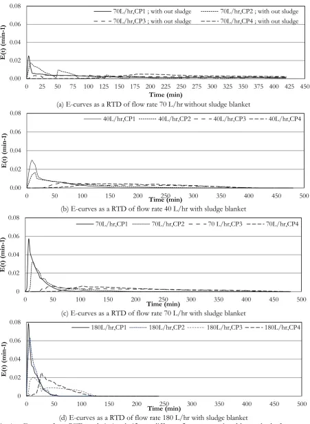
Fig. 4. E-curves from RTD study in jet clarifier at different flow rates analyzed by method of moments and the compartment model.

Figure 4(a) illustrates the RTD result of flow rate 70 L/hr without sludge blanket. Once tracer was feed into reactor, the probe at CP1 was detected the first inlet as plug flow behavior at 3 minutes. After the tracer flow pass CP1, it divided into two directions. The first part flowed consecutively to CP2 at 6 minutes,

0.00 0.02 0.04 0.06 0.08

0 25 50 75 100 125 150 175 200 225 250 275 300 325 350 375 400 425 450

E(t)

(

mi

n-1)

Time (min)

70L/hr,CP1 ; with out sludge 70L/hr,CP2 ; with out sludge 70L/hr,CP3 ; with out sludge 70L/hr,CP4 ; with out sludge

0.00 0.02 0.04 0.06 0.08

0 50 100 150 200 250 300 350 400 450 500

E(t)

(

mi

n-1)

Time (min)

40L/hr,CP1 40L/hr,CP2 40L/hr,CP3 40L/hr,CP4

0 0.02 0.04 0.06 0.08

0 50 100 150 200 250 300 350 400 450 500

E(t)

(

mi

n-1)

Time (min)

70L/hr,CP1 70L/hr,CP2 70 L/hr,CP3 70L/hr,CP4

0 0.02 0.04 0.06 0.08

0 50 100 150 200 250 300 350 400 450 500

E(t)

(

mi

n-1)

Time (min)

which also had plug flow behavior. Another part bypassed to CP3 as the tracer can be detected after 12 minutes. The first part at CP2 then returned downward following the flow pathway and, again, divided into two paths, including (1) flowed to CP1 and then recirculated between CP1 and CP2; (2) went to CP3 at 27 minutes (15 minutes after the bypass flow). All tracers at CP3 can flow to CP4 as the signal can be detected after 100 minutes.

With the sludge blanket at the same flow rate of 70 L/hr (Fig. 4(c)), the flow pattern was quite similar to the case without the blanket. However, some differences can be observed. First, the bypass flow from CP1 to CP3 was much decreased with the sludge blanket. This could be seen at 30 minutes as the bypass peak at CP3 was very small comparing to Fig. 4(a). The second difference was the reduction of the recirculation from CP2 to CP1. No looping peak at CP2 can be observed with the presence of sludge. The sludge blanket can restrict the bypass from CP1 to CP3 and the circulation of CP2 back to CP1. In addition, the liquid flow rate also influenced the bypassing. As can be seen in Fig. 5(d), there was a bypass peak at 12 minutes for 180 L/hr liquid flow rate, while the peak did not appear at 40 L/hr. Therefore, increasing the flow rate could induce more bypass flow.

Table 5. Mean residence time and of each flow rate. Flow

rate (L/hr)

Check point

Theoretical mean residence time

(min)

Experimental mean residence time at operating

without sludge (min)

Experimental mean residence time at

optimum condition (min) uL

D

40

1 2 - 13

0.11

2 55 - 71

3 170 - 172

4 364 - 203

70

1 1 137 8.5

0.16

2 32 108 41

3 97 188 182

4 208 260 200

180

1 0.5 - 12

0.48

2 12 - 13

3 38 - 43

4 81 - 42

Table 5 displays the RTD experimental mean residence time and variance. The tm were obviously

greater than the theoretical one due to the recirculation in reactor. It should be noticed that at flow rate of 180 L/hr, the residence times at CP3 and CP4 were very close. Since the tm of CP3 was the average value

from the bypass from CP1 and the recirculation between CP1 and CP2, the mean residence time should be higher than expected value. The appearance of bypass peak at CP4 also resulted in lower tm value.

Furthermore, the values in this study were in the range of 0.1 – 0.5 indicating the plug flow condition as the value was close to zero. The jet clarifier under the applied conditions can be considered as a plug flow reactor with partly mixed flow. The mixed flow regime can be enhanced by raising the flow rate as the was increased. In detail, the flow pattern was diagnosed as the plug flow at CP1 to CP2 and then changed to the mixed flow at CP3 to CP4. This pattern was consistent with the mechanism of the jet clarifier with sludge recirculation [23]. However, the difference in the mean residence time between the experimental and theoretical values had to be mentioned. This could be a result of short circuit or bypass flow. To prove this discussion, the mass balance of flow in these check points was constructed with the supposed flow pattern in Figs. 5 and 6.Once the liquid feeding (For QL) was introduced into the reactor, it

passed CP1 and divided to CP2 and CP3 denoted as QD and QB with the quantities of a and b, respectively.

The liquid that passed CP2 also separated into 2 paths including c (QR) back to CP1 and direct flow d (QJ)

Fig. 5. Flow pattern in jet clarifier reactor. Fig. 6. Ways followed by the tracer inside the reactor.

Using this flow pattern and the assigned quantities, the mass balance equation between each point can be expressed as in Eq. (10) - (17). Unfortunately, this mass balance equation cannot take the dead zone of the system into account since the outlet tracer quantity at CP4 was used for solving these equations.

CP1 = a + b (10)

CP1 = F + c (11)

CP2 = c + d (12)

CP2 = a (13)

CP3 = b + d + r (14)

CP4 = CP3 – r (15)

F = b + d (16)

F = CP4 (17)

The quantities of each variable were correlated from area under the curve between concentration and time, which resulted in amount of tracer passing that point divided with liquid flow rate. Since the flow rate in reactor was constant, using the area to represent the quantities of flow passing each check point was reasonable. After solving Eq. (10) to (17), the fractions of flow between each check point were summarized in Table 6.

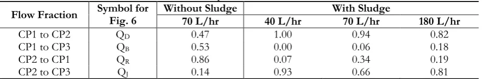
Table 6. Fraction of flow between each checkpoint.

Flow Fraction Symbol for _{Fig. 6} Without Sludge _{70 L/hr 40 L/hr} With Sludge _{70 L/hr 180 L/hr}

CP1 to CP2 QD 0.47 1.00 0.94 0.82

CP1 to CP3 QB 0.53 0.00 0.06 0.18

CP2 to CP1 QR 0.86 0.07 0.34 0.19

CP2 to CP3 QJ 0.14 0.93 0.66 0.81

From Table 6, the jet clarifier without sludge blanket had very high fraction of return from CP2 to CP1 (0.86) and also high bypass fraction from CP1 to CP3 (0.53). However, the return and the bypass fractions were respectively decreased to 0.34 and 0.06 for the same flow rate with sludge blanket in the reactor. The presence of sludge blanket can restrict the flow pathway and reduce the bypass and liquid recirculation resulting in the flow pathway similar to the design. Moreover, effects of flow rate can be clearly seen. At the flow rate of 40 L/hr, there was no bypass but it would get higher fraction as flow rate increased. Therefore, increasing flow rate can induce the bypass flow in reactor.

To enhance the turbidity removal, the increase of the flow rate to promote more recirculation should be considered. However, it could be compensated with the increased bypass flow. One should keep in mind that the increased of flow rate also resulted in shorter retention time, thus resulting in lower removal efficiency as the settling time could be insufficient [24]. In order to achieve the effective removal of turbidity, these factors have to be optimized.

QL

QD = QL - QB

QL

QR

QJ = (QL – QR)+QB

4.

Conclusion

The results indicated that jet clarifier was effective for removing colloidal particles and suspended solids from water. The optimal conditions for the turbidity removal were found as summarized in Table 7. Under the optimal condition, the turbidity removal efficiency of 80% was obtained.

It could be suggested that the jet clarifier could be applied instead of the conventional process since it requires less operating time and energy as well as smaller area but can provide similar efficiency as the conventional coagulation at the same overflow rate. The settling efficiency could be also enhanced by applying a settling plate or tube, which should be further studied in the future.

Table 7. Summary of the optimal design criteria of the jet clarifier with 25 cm sludge height.

Liquid flow rate

(L/hr)

Coagulant type

Chemical dose

(mg/L) Mechanism

G (s-1₎

t

(s) (G•t) (hr) seda (hr) Jetb

70 aluminium _sulphate 20 – 30 _flocculation coagulation 564.32 _{0.743 1800} 1.89 1068.47 _1337.40 2.79 3.29

Remarks: a) Retention time of the sedimentation zone; b) Retention time of the Jet clarifier.

From the RTD results, the jet clarifier under the applied conditions contained the plug flow reactor pattern in the coagulation zone and changed to a mixed flow pattern in the flocculation and settling zones. The increase of flow rate can enhance the recirculation resulting in the increased efficiency. However, this could lead to more bypass flow and shorter retention time, which would reduce the process performance. In addition, the presence of a sludge blanket plays a key role in the separation since it helped controlling the flow pattern as well as increasing a target for particle agglomeration.

It is a well-known fact that flow patterns strongly depend on flow rate. However, at the scale of this experimental device, the flow convective contributionsinduced by flow rate can greatly affect the flow pattern. In addition, shape and size of a buffer installed in a reactor can also influence the efficiency. The study in detail should be conducted on its effects on flow behavior and treatment efficiency. This could lead to the optimization of the operation for improved efficiency.

5.

Nomenclature

Ci = Initial turbidity (NTU)

Cf = Final turbidity (NTU)

 = Liquid density (kg/m3₎

s = Particle or floc dencity (kg/m3)

C = Floc volume concentration

 = Dynamic viscosity of liquid (kg/m._s)



Acknowledgements

This work was financed by the Chulalongkorn University Fund, Department of Environmental Engineering, Faculty of Engineering, Chulalongkorn University.

References

[1] G. Degremont, Water Treatment Handbook, vol. 2, 6th _{ed. France: Lavoisier Publishing, 1991.}

[2] I. C. Tse, K. Swetland, M. L. Weber-Shirk, and L. W. Lion, “Fluid shear influences on the performance of hydraulic flocculation systems,” Water Research, vol. 45, pp. 5412–5418, 2011.

[3] S. R. Qasim, E. M. Motley, and G. Zhu, “Coagulation,flocculation and precipitation,” in Water Works Engineering: Planning, Design, And Operation. New Jersey, USA: Prentice Hall, 2000, pp. 229–300.

[5] A. H. Essadki, B. Gourich, Ch. Vial, and H. Delmas. “Residence time distribution measurements in an external-loop airlift reactor: Study of the hydrodynamic of the liquid circulation induce by the hydrogen bubles,” Chemical Engineering Science, vol. 66, pp. 3125–3132, 2011.

[6] A. Bittante, J. García-Serna, P. Biasi, F. Sobrón, and T. Salmi, “Residence time and axial dispersion of liquids in Trickle Bed Reactors at laboratory scale,” Chemical Engineering Journal, vol. 250, pp. 99–111, 2014.

[7] Y. Gao, F. J. Muzzio, and M. G. Ierapetritou, “A review of the Residence Time Distribution (RTD) applications in solid unit operations,”Powder Technology, vol. 228, pp. 416–423, 2012.

[8] A. T. Harris, J. F. Davidson, and R. B. Thorps, “Particle residence tine distribution in circulating fulidise beds,” Chemical Engineering Science, vol. 58, pp. 2181–2202, 2003.

[9] Performance Statistic of Water Quality. [Online]. Available:

http://www.mwa.co.th/ewtadmin/ewt/mwa_internet _eng/ewt_news.php?nid=97 [Accessed: Dec 2011].

[10] D. Bouyer, C. Coufort, A. Linéa, and Z. Do-Quang, “Experimental analysis of floc size distributions in a 1-L jar under different hydrodynamics and physicochemical conditions,” Journal of Colloid and Interface Science, vol. 292, pp. 413–428, 2005.

[11] S. Kawamura, Integrated Design and Operation of Water Treatment Facilities, 2nd _{ed. USA: John Wiley & Sons,}

INC, 2000.

[12] T. D. Reynolds and P. A. Richards, Unit Operations And Processes In Environmental Engineering, 2nd _ed.

USA: PWS Publishing Company, 1996.

[13] APHA, AWWA, and WEF, Standard Methods for the Examination of Water & Wastewater, 21st _ed.

Washington, DC: American Public Health Association, 2005.

[14] The Designing of Static Mixer (Noritake) In Rapid Mix for Water Treatment. [Online]. Available:http://www.tumcivil.com/engfanatic/content/upload/File/mwa/sta_000e.pdf [Accessed: Jan 2012].

[15] M. A. Hughes, “Coagulation and flocculation Part 1-2,” in Solid-liquid separation, 4th _{ed. L. Svarovsky,}

Eds. Pondicherry, India: Integra Software Services Pvt Ltd., 2000, pp. 104–165.

[16] H. S. Fogler, Elemrnts of Chemical Reaction Engineering, 4th _{ed.USA:Pearson Education, 2013.}

[17] O. Levenspiel, Chemical Reaction Engineering, 3rd _{ed. USA: John Wiley & Sons, 1999.}

[18] R. M. Alkhadder, P. R. Higgins, D. A. Phipps, and R. Y. G. Andoh, “Residence tine distribution of a model hydrodynamic vortex separator,” Urban Water, vol. 3, pp. 17–24, 2001.

[19] R. Chamnanmor, P. Painmanakul, and C. Puprasert, “Study of in-line coagulation and flocculation processes for turbidity removal: Experimental approaches,” in Proc. The 5th AUN/SEED-Net Regional Conference on Global Environment, Bundung, Indonesia, 2012, p. 25.

[20] Samsen Water Treatment Plant, “Water Quality Report, Report of the water quality analysis system,” MWA, Bangkok, Thailand, 2009-2012.

[21] Samsen Water Treatment Plant Engineering Group, “Existing design capacities and loadings report of the Samsen Water Treatment Plant Engineering Group,” MWA, Bangkok, Thailand, 2002.

[22] P. R. López, A. G. Lavín, M. M. M. López, and J. L. B. de las Heras, “Flow models for rectangular sedimentation tanks,” Chemical Engineering and Processing, vol. 47, pp. 1705–1716, 2008.

[23] S. D. Lin, Water and Wastewater Calculations Manual, 2nd _{ed. USA: The McGraw-Hill, 2007.}