Philip J. Platts
Abstract. Traditionally, community models have focused on density-dependent factors. More recently, though, studies that consider populations interacting on a spatial (as well as temporal) scale have become very popular. These metacommunity models often use the patch-occupancy approach, where the focus is on regional dynamics (patches are classified as simplyoccupiedor vacant). A few studies have extended this work by modelling local dynamics explicitly, although the food webs involved have been relatively simple. This paper takes the next step and considers a spatially explicit habitat where species interact across three trophic levels. The aim is to investigate how web connectance, patch abundance and dispersal patterns affect a community’s ability to recover from the loss of a species. I find that asynchrony among patch dynamics may arise from relatively low rates of migration, and that the inclusion of space significantly reduces the risk of cascading extinctions. It is shown that communities with sparsely connected food webs are the most sensitive to perturbations, but also that they are particularly well stabilised by the introduction of space. In agreement with theoretical studies of non-spatial habitats, species holding the highest trophic rank are the most susceptible to secondary extinctions, although they often take the longest to die out. This is particularly pronounced in spatial habitats, where the top predator appears to be the least well adapted to exploit the stabilising properties of space. Results such as these are discussed in detail, and their implications are set in the context of habitat management.
Citation: Platts PJ (2004). A Patchy Approach to Food Web Persistence. MRes Thesis, University of York, UK and Link¨oping Universitet, Sweden
Date: August, 2004.
1. Introduction
It is often instantly apparent that space is fundamental to species’ interactions; the positioning of an individual sessile organism, for example, strongly influences with whom it must compete. The literature is rich with empirical studies of such organisms, their immobility making reliable data collection a relatively simple task. When studying communities of highly mobile organisms, however, consideration of spatial processes brings with it both practical and theoretical compli-cations. Some degree of spatial structure is apparent in all natural communities, yet for a long time the general opinion was that the inclusion of space in a theoretical model might obsure more than inform. Instead, the vast majority of ecological modelling during the 20thcentury concerned itself with density-dependent factors, assuming no spatial element. Such work has been invaluable in providing insights into local community interactions and demographics, and is vital in laying the foundations for a larger scale approach. In recent times, however, it has become increasingly apparent that if we are to make true headway in unravelling nature’s processes then the role of space can no longer be ignored, particularly in view of the ever increasing demand for scientific guidance on environmental issues.
Over the past 15 years, the potential of metapopulation models to shed light on ecological pro-cesses has been rapidly realised1, though the idea is not a new one. As early as the 1930s, examples were emerging of how considering space might provide new clues, previously obscured in the haze of panmictic population models. Gause (1935) observed the persistence of certain predator-prey communities in the wild, but could not promote similar stability in the laboratory: wild fluctuations in population densities invariably led to extinctions. Gause suggested that in a natural setting populations might be spread across an ensemble of spatially distinct local commu-nities; so long as dynamics were asynchronous among patches, localised drops in population could perhaps be countered by reinvasion from neighbouring communities, thus promoting long-term coexistence. Experimental studies in the 1950s (Andrewartha and Birch 1954; Huffaker 1958) vindicated Gause’s conjectures, although it was not until the works of Levins (1969, 1970) that the metapopulation paradigm was formalised.
Levins’s classic patch-occupancy model considers space implicitly, focussing simply on the propor-tion of occupied patches resulting from a uniform distribupropor-tion of migrants. Extensions of this work have included metacommunity models (see Leibold et al. 2004), and also spatially explicit mod-els, whereby dispersal is localised and the flickering mosaic of occupied sites is followed through time (see Tilman and Kareiva 1997). In this paper, inspiration is taken from such frameworks, although here the number of inhabitable patches is limited to a spatially discrete few (to be varied) positioned randomly across a lattice. The aim is not to question how the spatial distribution or frequency of patches might arise — it is assumed that the metacommunity is already well estab-lished — but rather to investigate the robustness of regional persistence.
The populations within each patch are modelled explicitly using a tri-trophic web of interactions. Consequently, more than one species may coexist locally and population densities may vary from patch to patch. This can lead to complicated dynamics (Nee et al. 1997), but this does not discourage since cyclic and chaotic solutions may be consistent with natural coexistence (Hastings 1988). In fact, similar models have used cyclic dynamics to great effect. For example, Ranta et al. (1997) successfully predicted fluctuations in Canadian lynx populations, the results of their spatially linked population model striking a strong resemblance to the empirical data. The fact that local population densities may fluctuate rather than settling to equilibrium values can often promote coexistence in spatially explicit predator-prey models: spatially shifting refuges serve both to prolong persistence of inferior competitors as well as to provide temporary respite for prey (Jansen 1995; Tilman and Kareiva 1997). Of course, the level of dispersal is an important factor in promoting such coexistence: too little and local populations could not be rescued from
1Using figures from the BIOSIS database, Hanski and Gilpin (1997) graph a dramatic rise in the number citations
extinction; too much and patch dynamics may be synchronised, allowing a particular species to become extinct simultaneously in all patches (Hollyoak and Lawler 1996).
The idea that asynchrony among patch dynamics prolongs regional coexistence is not, in itself, much of a revelation. What is important is that patchy habitats have been observed in natural settings and thus we must query under what conditions such heterogeneity might arise (de Roos and Sabelis 1995). In an attempt to answer this question, I begin with the null state that all species persist in all patches and that their local dynamics are synchronised. Migration is then introduced using a model that expresses dispersal as a function of both distance and patch abun-dance. Once the system has settled, the robustness of regional persistence is determined via the forced removal of one species. In particular, the frequency of cascading extinctions is compared for different levels of patch abundance, dispersal and web connectance. Results for a single-patch community are also discussed for comparison.
2. Methodology
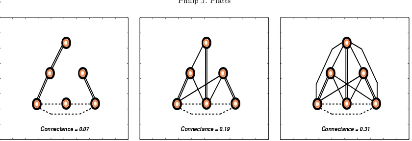
2.1. Local Dynamics. Each patch is inhabited by six species, coexisting across three trophic levels. The food web is triangular in structure2, with three basal species (autotrophs requiring no explicit food source for persistence) holding the lowest trophic rank. These are consumed by two intermediate species, which are prey for the one top species. Omnivory is also allowed when web connectance is suitably high.
The interactions within each patch are described by the generalised Lotka-Volterra equations:
dNi
dt =Ni
ri+
6
X
j=1
αi,jNj
for species i= 1, . . . ,6, (1)
wheredNi/dtis the rate of change of density with respect to time,ri is the intrinsic growth rate andαi,jrepresents the effect of speciesj on the per capita rate of increase of speciesi. For a given
web connectance3, the appropriate number of consumer-resource links are randomly allocated po-sitions in the web, the only proviso being that every consumer must prey on at least one species in the trophic level directly beneath. Research concerning the relative strengths of species inter-actions is still in its infancy. However, empirical evidence to date strongly suggests that generalist consumers tend to favour just a few of their many possible prey species (see McCann 2000 for a review, or Wootton 1997 for an example). In an attempt to mimic this skewed distribution of interaction strengths, each predator is randomly assigned one strong feeding link, whilst the other links are assumed to be weak. Figure 1 shows three possible web configurations: the first has the lowest possible connectance; the second has a medium level of connectance and the third shows an example where all links are present.
2.2. Regional Dynamics. Each patch is continually subject to migration events: per time unit, a fixed proportion, m, of each species’ population migrates from its current patch and disperses among the neighbouring communities. For a habitat of s patches, the number of individuals migrating from patchqto patchp, per unit time, is given by (Hanski and Woiwod 1993)
Mi,p,q =mNi,q e
−dp,q/c
Ps
l,l6=qe−dl,q/c
fori= 1, . . . ,6, (2)
whereNi,q is the density of speciesiin patchq, the distance between the two patches isdp,q, and cis a parameter. Thus the flow of migrants is greatest between patches a relatively small distance apart (the strength of this bias is determined by c: lower values correspond to more localised
2Triangular communities are often found in real food webs, see for example Cohenet al.’s recent survey of a
lake ecosystem (2002).
O
O
O
O
O
O
o
o
o
o
o
o
Connectance = 0.07
O
O
O
O
O
O
o
o
o
o
o
o
Connectance = 0.19
O
O
O
O
O
O
o
o
o
o
o
o
[image:4.595.93.513.77.221.2]Connectance = 0.31
Figure 1. Web diagrams show three viable configurations for between-species local interactions. The dashed lines connecting the three basal species represent direct interspecific competition (present in all webs), whilst the solid lines rep-resent consumer-resource links: single for a weak link; double for a strong link. The first diagram illustrates that the lowest connectance does not permit multiple resource links, and hence all predator-prey interactions are strong. The second shows an example of a configuration for an intermediate connectance and the third an example where all possible interactions are present.
dispersal). The change then, per unit time, in patchpdensities as a result of migration is given by
e Ni,p=
s X
q q6=p
Mi,p,q
| {z }
Flux in
−mNi,p | {z }
Flux out
fori= 1, . . . ,6. (3)
Theq 6=pcondition on the summation term means that no migrant may return to the patch it has just vacated. Migration events are instantaneous and, as such, all individuals are continually subject to the competitive interactions described by Equation (1):
dNi,p
dt = (Ni,p+Ni,pe )
ri+
6
X
j=1
αi,j(Nj,p+Nj,pe )
fori= 1, . . . ,6. (4)
The dispersal rule used here ensures that all migrants are successful in reaching another patch. It is plausible, however, that migration might pose some kind of risk to the individual, and that this risk should increase with the distance travelled. This possibility was tested by multiplying Equation (2) by the term (1−τ dp,q), where 0< τ <1 quantifies the risk. However, for realistically small values ofτ, the results are qualitatively similar to the original model and are therefore not described here.
2.3. Parameters. All migration and growth rates are defined per day and hence the time variable relating to Equations (1) through to (4) should be interpreted similarly. The parameters to be varied are: patch abundance (s= 1 tos= 17); the migration coefficients (m= 0.001 tom= 0.1;
c= 0.1 toc = 1) and web connectance (C= 0.07 to C= 0.31). Intrinsic growth rates are fixed at 1, -0.01 and -0.001 for the basal, intermediate and top species respectively. To give meaning to these values, an example of estimated generation times is given4: one day for basal species; 26 days for intermediate species and 318 days for the top species. If no interaction exists between two species thenαi,j is set to zero; otherwise, the strength of the link is drawn at random from a continuous uniform distribution, the limits of which are outlined below.
4Generation times are estimated from allometric relations between mortality rates and body size (Roff 1992),
Predation Coefficients. If a consumer has only one prey then the feeding link is assumed to be strong, its value being drawn from the interval -(0, 0.5]. Otherwise, the one randomly selected strong link is assigned a value from the interval -(0, 0.4], whilst all weak links are assigned values from -(0, 0.1]/(number of prey - 1). Hence the average link strength is negatively correlated with the number of prey species (McCannet al. 1998).
Prey Coefficients. The effects that prey have on their predators are given byαj,i=−eαi,j, where eis the conversion efficiency (0.02 for omnivorous links, 0.2 otherwise). Thus predator-prey inter-actions are strictly asymmetric and no mutualistic relations exist within the system.
Direct Interspecific Competition. Basal species compete with one another for the implicit resource that fuels their growth. The strength of these links are drawn from the interval -(0, 0.5]. There is no direct interspecific competition within higher trophic levels, although indirect competition exists implicitly between consumers that share a common resource.
Intraspecific Competition. All individuals are subject to within species competition, the self-limitation terms,αi,i, being drawn from the interval -(0, 1].
The competitive interaction strengths defined here are based on those used by Ebenmanet al. in their study of how single-patch communities respond to species loss (2004).
2.4. Generating Starting Communities. The global habitat is a 25 cell by 25 cell grid, in which the patches are allocated their positions at random from a continuous uniform distribution. Initially, the conditions for each distinct local community are identical: a permanent single-patch starting community is found (see Appendix A for details) and replicatedstimes. Migration is then introduced and the system, starting from equilibrium values, is integrated over 20,000 time units (this equates to approximately 55 years). This gives the opportunity for spatial heterogeneity to emerge and the system time to settle. Since I am interested in the deterministic behaviour of the system, no restrictions are made on how large a population might become (competition for space is not considered). However, a lower bound is imposed, below which a species’ patch density is considered too small to avoid stochastic extinction. This threshold is set at
0.05 × min{Ni,p|t=0: i= 1. . .6; p= 1. . . s}, (5)
that is, five percent of the smallest starting density. During integration, local densities are checked to see whether they have fallen below this threshold and, if so, they are set to zero. Only if no local extinctions have occurred after 20,000 time units are the final densities accepted as a viable starting community; otherwise, new interaction coefficients and patch layout are generated and the process is repeated until a persistent community is found.
In the majority of cases, the system settles well within the allotted time. Occasionally though, the inclusion of the non-linear migration terms give rise to heteroclinic cycles, where three or more species’ densities oscillate with increasing amplitude over time. The ultimate extinction of at least one of the species is inevitable, although since the period of the oscillations increases over time it sometimes takes a while before the extinction threshold is breached. It is for this reason that the system is integrated over such a long time period: it is the asymptotic state of the system that is of interest and therefore all destabilising transients must be lost before the integration is halted.
2.5. Species Removal. In order to investigate how dispersal and patch abundance affect meta-community stability, the system is perturbed by a forced extinction event: species i is removed from the starting community in all patches. That is, the species’ global density is set to zero, leaving no means by which it might recover. The model is then integrated over 20,000 time units and the final densities are recorded. This procedure is repeated 150 times for each species,i= 1 to
levels. For each new run performed, a new starting community is constructed, as outlined above.
The removal of a species is a convenient means by which to assess the robustness of coexistence in spatial habitats. More than this, though, species extinctions are a very real occurrence and so it is hoped that this approach provides some insight into how real ecosystems might respond to species loss. To add realism to the model,if all resources on which a consumer usually feeds are lost then the consumer forages for any available source of prey. In terms of the simulations, this means that the consumer is allocated one weak (non-cannibalistic) feeding link at random (the ‘foraging link’). Thus, whilst its chances of survival are still low, global extinction is not a certainty. Although this adaptability of endangered species has not been included in earlier (theoretical) work regarding species loss, Kondoh (2003) finds that a consumer’s adaptive food choice is key to the long-term stability of complex communities.
3. Results and Discussion
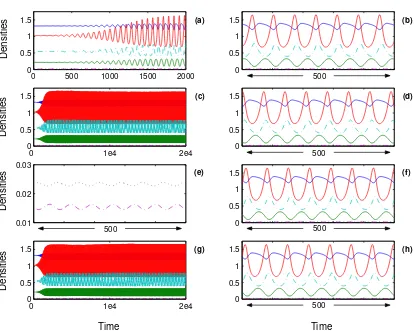
3.1. The Introduction of Space. Before looking at how well the communities fared when per-turbed by species removal, it is appropriate to draw attention to a couple of interesting results from the community assembly process. In general, the introducion of migration has only a slight effect on local dynamics and the densities soon settle to equilibrium values. There are, however, two exceptions that warrant further discussion. The first arises when the permanent local com-munities contain a stable limit cycle: migration causes the phase space trajectories to spiral away from the interior fixed point and toward the limit cycle. Consequently, all species’ densities ex-hibit self-sustained oscillations in all patches. Figure 2 gives an example of this phenomenon in an eight-patch habitat with a migration rate of one percent per day. Despite the identical initial conditions, the effect of localised migration is to desynchronise oscillations from patch to patch. Thus, Figure 2 gives a clear example of how spatially shifting refuges for prey can arise, even when the rate of migration is very low.
0 500 1000 1500 2000 0
0.5 1 1.5
Densities
0 0.5 1 1.5
0 1e4 2e4
0 0.5 1 1.5
0 0.5 1 1.5
0.01 0.02 0.03
0 0.5 1 1.5
0 1e4 2e4
0 0.5 1 1.5
0 0.5 1 1.5
500
500
500
500 500
(a)
(c)
(e)
(g) (h)
(f) (d) (b)
Time Time
Densities
Densities
[image:7.595.95.509.85.416.2]Densities
Figure 2. Following the introduction of migration between eight identical patches, population densities are followed over a period of 20,000 time units. The solid lines track the basal species’ densities; the dashed track the intermedi-ate, whilst the dotted line tracks the top species. For clarity, six of the patches show zoomed perspectives of their dynamics: patch (a) focuses on the first 2,000 time units; patches (b), (d), (e), (f) and (h) all focus on the last 500, by which time the system has settled to reveal stable asynchronous oscillations. The web connectance is 0.19 and the migration coefficients arem= 0.01 andc= 0.4.
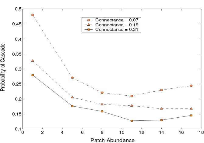
3.2. The Risk of Cascading Extinctions. In Figure 3, the probability that a primary extinc-tion event leads to the global loss of at least one further species is compared for different patch abundances. Results for the single-patch habitat are consistent with those found by Ekl¨of and Ebenman (unpublished manuscript). Since their food web structure and interaction strengths are similar to those used here, the similarity with their results indicates that the foraging ability of an endangered species (described in Section 2.5) rarely prevents its extinction in this case. Single-patch results also match closely with those found by Lundberg et al. (2000) and Frodin et al. (2002). This is more surprising because both these studies investigate a highly connected linear web. Thus, the similarity in extinction probabilities suggests that separating the six species into a vertical hierarchy of interactions has surprisingly little effect on their ability to coexist. It is noteworthy, though, that this is only true when web connectance remains high and that a decrease in the frequency of vertical interactions significantly increases the risk of secondary extinctions.
0 2 4 6 8 10 12 14 16 18 0.1
0.15 0.2 0.25 0.3 0.35 0.4 0.45 0.5
Patch Abundance
Probability of Cascade
[image:8.595.134.469.85.319.2]Connectance = 0.07 Connectance = 0.19 Connectance = 0.31
Figure 3. How does the risk of cascading extinctions vary with patch abundance? The results shown are for migration coefficients ofm= 0.01 andc= 0.4.
Table 1. Chi-square tests show highly significant differences between the single-patch and five-single-patch habitats (m= 0.01;c= 0.4). Frequencies are the number of cascading extinction events following species removal in 900 runs.
Connectance 1-Patch 5-Patch χ2 Result p-value (1 d.f.) 0.07 419 244 72.2931 <0.0001 0.19 295 185 33.7528 <0.0001 0.31 259 159 30.5393 <0.0001
stabilising effect is most pronounced in the transition from one to five patches, although the ex-tinction probabilities continue to decrease for the eight and 11-patch habitats. The robustness of this result is amplified by the fact that community assembly is deliberately biasedagainst the emergence of spatial heterogeneity: the (identical) permanent local communities are resilient to disruption by migration which, compared with other models using a similar dispersal rule (Han-ski et al. 1993; Ranta et al. 1995, 1997), is set very low. Whilst, in general, the differences in pre-extinction patch densities are indeed only slight, it is clear that they significantly increase the system’s ability to recover from a major perturbation.
Table 2. Chi-square tests do not show significant differences between the 11-patch and 30-11-patch habitats (m= 0.01;c= 0.4). Frequencies are the number of cascading extinction events following species removal in 900 runs.
Connectance 11-Patch 30-Patch χ2 Result p-value (1 d.f.)
0.07 189 179 0.2767 0.5989
0.19 160 151 0.2488 0.6180
0.31 115 117 0.0049 0.9440
is particularly intriguing because the dispersal rule they use is similar to Equation (2). One ex-planation for the differences in our results could be the foraging link included here. However, it is hard to see how this alone could negate a sudden reduction in stability for high patch abundance, especially considering Frodin et al. use a higher web connectance than two of the examples in Figure 3. A more plausible reason why the tri-trophic system proves more stable is that, although migration ratesper day are equal for all trophic levels, the proportion of individuals migratingper generationcan differ (due to the different life expectancies). Therefore, species at different trophic levels can be considered to experience their worlds at different spatial, as well as temporal, scales. As shown by Chesson and Huntly (1997), coexistence can be promoted by populations’ disparate exploitation of spatio-temporal heterogeneity.
In all cases, the risk of cascading extinctions is higher in habitats with a lower web connectance. It is thought that, unless their effects are dampened by weak interactions, strong consumer-resource links have an adverse effect on community level stability (see McCann 2000). For the lowest connectance used here, all consumer-resource links are assumed to be strong (see Figure 1). As connectance increases, so too does the frequency of weak links to alternative prey items, causing an overall reduction in the mean interaction strength. It is therefore not surprising that systems with a higher web connectance are found to be less prone to collapse. The possible instabilities in habitats with an intermediate web connectence (discussed in Section 3.1) are not exposed for the low migration rate used here and, in any case, such configurations would be weeded out in the selection of starting communities. Although the number of interactions is linearly related to con-nectance, the differences between extinction probabilities attenuate with increasing connectance. Thus, the relationship between connectance and the ability of weak interactions to stabilise the system appears to be non-linear in this model. Whether or not this is a general result is not clear: the existence of skewed interaction strengths is a relatively recent finding and its effects have yet to be fully understood.
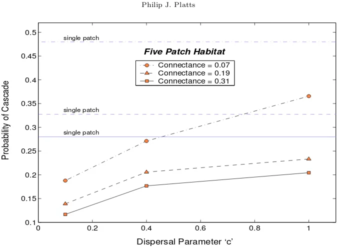
3.3. Dispersal Patterns. Any asynchrony among local dynamics is a direct consequence of lo-calised dispersal. Thus the degree to which migrants are inclined to settle in nearby patches is clearly central to promoting, or inhibiting, regional coexistence. To investigate just how sensitive the model is to different patterns of dispersal, c is varied between sufficiently large bounds to expose all significant variation in the frequency of cascading extinctions. There is no doubt that dispersal abilities can vary enormously from species to species, and therefore this also serves to encompass a wider variety of natural communities into the scope of the model.
0 0.2 0.4 0.6 0.8 1 0.1
0.15 0.2 0.25 0.3 0.35 0.4 0.45 0.5
Connectance = 0.07 Connectance = 0.19 Connectance = 0.31
Five Patch Habitat
Dispersal Parameter ‘c’
Probability of Cascade
single patch
single patch
[image:10.595.133.473.73.321.2]single patch
Figure 4. Shows how increasing the dispersal distance of migrants affects the risk of cascading extinctions following the loss of a species. The horizontal lines mark the probabilities from the single-patch model. The results shown are for a five-patch habitat (m= 0.01); refer to Appendix B for more detailed results and higher patch abundances.
therefore the system would be deterministically identical to the non-spatial model.
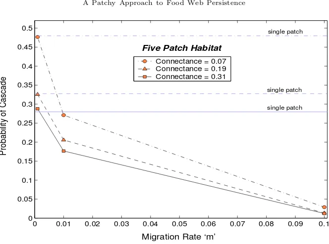
3.4. The Rate of Migration. Figure 5 shows the risk of cascading extinctions for three differ-ent migration rates in a five-patch habitat. As for the dispersal patterns, results for higher patch abundances can be found in the Appendices, although they are qualitatively similar to those de-scribed here. For the lowest rate investigated (0.1 percent per day), the extinction probabilities are similar to those for the single-patch model. This is true for all levels of connectance and patch abundance (see Appendix C). The dramatic decrease in extinction probabilities when the rate is increased to one percent suggests a threshold between m= 0.001 and m= 0.01 where migrants become numerous enough to create differences in patch dynamics. Another reason for this large drop in the risk of cascading extinctions is the nature of the extinction threshold, described by Equation (5); any efforts by migrants to recolonise a patch where a species has become locally extinct will be unsuccessful, unless the propagule size (the density of the ‘rescue party’) is greater than the extinction threshold.
0 0.01 0.02 0.03 0.04 0.05 0.06 0.07 0.08 0.09 0.1 0
0.05 0.1 0.15 0.2 0.25 0.3 0.35 0.4 0.45 0.5
Migration Rate ‘m’
Probability of Cascade
Connectance = 0.07 Connectance = 0.19 Connectance = 0.31
Five Patch Habitat
single patch
[image:11.595.136.468.75.322.2]single patch single patch
Figure 5. Shows how increasing the rate of migration affects the risk of cas-cading extinctions following the loss of a species. The horizontal lines mark the probabilities from the single-patch model. The results shown are for a five-patch habitat (c= 0.4); refer to Appendix C for more detailed results and higher patch abundances.
is hard to make comparisons with previous work. However, Kondoh (2003) models fluctuations in link selection and predicts patterns of interaction consistent with empirical observations. Secondly, consumers surviving with the foraging link are likely to have particularly low densities. Although this model focuses on the deterministic behaviour of the system, it must not be forgotten that populations persisting at lower densities are more prone to extinction in the presence of demo-graphic stochasticity (Engen 1998; Ebenmanet al. 2004). Finally, a migration rate as high as ten percent can, in some cases, make the generation of stable starting communities very difficult, as explained in Section 3.1. This calls in to question how realistic such a high migration rate is for the kind of metacommunities described in this paper.
3.5. Trophic Position. The above discussion has generalised extinction events in two distinct ways. Firstly, in any particular run, the robustness of community persistence has been defined by the presence or absence of a cascade, rather than the frequency of secondary extinction events. Secondly, the trophic position of neither the removed species nor the species becoming subse-quently extinct has been considered explicitly. To address this, a closer look is now taken at the nature of secondary extinctions.
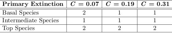
Table 3. Given that a cascading extinction has occurred, how many species are likely to be lost? This table shows the median number of secondary extinctions for the single-patch habitat. Median values for the spatial habitats are equal to one for all parameter values discussed.
Primary Extinction C = 0.07 C = 0.19 C = 0.31
Basal Species 2 1 1
Intermediate Species 1 1 1
Top Species 2 2 2
In any multi-tophic model, the basal species provide the foundations on which all other interactions are built. Thus, the removal of a basal species is likely to have particularly severe ramifications, as can be seen in Figure 6. For the lowest connectance, over half of the cascading extinction events recorded result from the loss of a basal species. For the two higher connectances, this proportion is larger still. This is because higher connectances allow omnivory and so both the top consumer and the primary consumers may rely on the basal species directly. This has a particularly large impact on the proportions in Figure 6 because the top species is the most prone to secondary extinction (see Figure 7). Despite the effects of ominivory, the median size of cascades caused by the removal of a basal species is smaller for higher connectances (Table 3), due to consumers relying on more than just one prey species.
The removal of an intermediate species frequently leads to secondary extinctions, either directly (when the top species loses its focal prey) or indirectly (when the competitive interactions beneath are disrupted). The latter is an example of when predator-mediated coexistence previously held prey densities in check, although this behaviour is found to be much less common. Similarly, it is rare that the loss of the top species causes extinctions lower down the food-chain (Figure 6), although when it does the consequences are often severe (Table 3): the absence of top-down reg-ulation releases intermediate species from predation, allowing them to over-exploit the resources on which they depend. In such cases, it is not uncommon for all but one or two species to be lost in the resulting cascade. Empirical evidence for such communitiy collapses is well known (Estes and Palmisano 1974, for example), although it has proved an elusive phenomenon to model. A patch-occupancy study by Caswell (1978) shows that predator-mediated coexistence may be con-siderably more probable in an open system. I find the introduction of space to have little effect on the proportions shown in Figure 6, although this is a consequence of the local dynamics — it has been known for some time that predator-mediated coexistence in closed Lotka-Volterra systems requires a delicate balance of interaction strengths (Cramer and May 1971).
Top Species Removed
Intermediate Species Removed
Basal Species Removed
Connectance = 0.07 Connectance = 0.19
Basal Species Removed
Intermediate Species Removed Top Species
Removed
Top Species Removed
Intermediate Species Removed
Basal Species Removed
[image:13.595.105.508.90.238.2]Connectance = 0.31
Figure 6. Pie diagrams show the proportions of cascades caused by the removal of a species at the different trophic levels. More runs were performed where a basal species was deleted, but this bias has been corrected in the calculation of these fractions. The results shown are for a single-patch community, although these proportions do not vary significantly with the introduction of space.
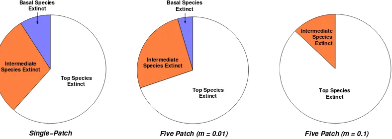
Whilst the top species is ultimately the most likely to be lost, its population invariably takes the longest of all species to fall below the extinction threshold. This result has important consequences for conservation efforts, because a top predator observed to have a stable population may actually be caught in a long, ultimately terminal, transient. In a system where the predator plays an important role in mediating competition beneath it, its unnoticed decline to extinction is likely to be followed by a relatively quick succession of extinctions among lower trophic ranks. This danger is even more apparent in spatial habitats, where asynchrony in local dynamics lengthens relaxation times still further and where the top predator is even more at risk (in comparison to lower order species — Figure 7).
Top Species Extinct Basal Species
Extinct
Intermediate Species Extinct
Single−Patch Five Patch (m = 0.01)
Intermediate Species Extinct
Top Species Extinct Basal Species
Extinct
Five Patch (m = 0.1) Top Species
Extinct Intermediate
Species Extinct
Figure 7. Pie diagrams show the proportions of secondary extinction events occurring at the different trophic levels. The bias towards extinctions at lower levels (caused by the triangular food web structure) has been corrected in the calculation of these fractions. The results shown are for a connectance of 0.31 and, for the latter two charts, a five-patch habitat withc= 0.4. Charts for lower connectances reveal a similar pattern, and are therefore not included here.
4. Concluding Remarks
[image:13.595.107.501.453.593.2]J. A. Thomas et al. 2004). The depletion of terrestrial and marine habitats has received much attention in recent times, but it is becoming increasingly apparent that freshwater systems are also at great risk; a study of North American freshwaters (Riciardi and Rasmussen 2000) predicts that, unless the hundreds of endangered species can be saved, future extinction rates could equal those of tropical forests. As a species, humans have a unique capacity to manipulate their en-vironment for short-term gains. If we are not wise then this ability to disrupt and exploit will undoubtedly end in irreparable damage and ultimately our own extinction. Untold damage has already occurred and we must now, more than ever, use our intelligence to gain understanding of ecological processes and help guide conservation efforts and habitat management.
Theoretical models such as this serve merely as metaphors for the awe-inspiring complexity that underpins natural processes. Nonetheless, when combined with empirical and experimental data, they are invaluable tools in highlighting possible consequences of disrupting previous stable ecosys-tems. Key to successful modelling is an awareness of how the simplifications introduced are likely to affect the system’s behaviour. It is remarkable, then, that until recently the role of space in ecological models has been so frequently omitted. This paper builds on the foundations laid by both non-spatial and simple patch-occupancy models. However, the explicit modelling of both local and regional dynamics has not been without some important assumptions.
Firstly, so as not to cloud the effects of migration, the starting communities are assembled by link-ing identical local communities by migration. In a natural settlink-ing, however, the structure of any local food web grows out of successive colonisation and extinction events (MacArthur and Wilson 1967; Holt 2002). Whilst modelling community assembly in a realistic manner would be difficult at best, it must be kept in mind that the chosen approach is likely to influence what conclusions are drawn from the model. Secondly, this paper does not attempt to model stochastic processes, and yet they clearly play an important role in any natural community. The short-term fluctua-tions in populafluctua-tions caused by births and death could perhaps be modelled by adding ‘noise’ to the local dynamics, although to be truely realistic the interaction strengths must also be subject to spatio-temporal variability. Such an extension of this model would certainly be interesting, although would itself require many new assumptions. Finally, the local dynamics are modelled using the generalised Lotka-Volterra equations. There are, however, a multitude of other ways to model competitive interactions and there is certainly no definitive guide to which might be most appropriate and when. A recent study by Lewis (2004) investigates the post-extinction commu-nities in closed systems for different types of functional response. An interesting result is that a Holling Type III response is less likely to allow the successful reinvasion of an extinct species than the Type I response employed here. This has obvious implications for spatial models, where local extinctions and subsequent (successful) reinvasions are common occurrences.
5. Acknowledgements
Appendix A: The Permanence Criterion
For a long time, ecologists have attacked the problem of assembling realistic community models by seeking those that yield an asymptotically stable fixed point. However, since its introduction by Schusteret al. in 1979, the concept of permanence (in the sense defined below) has given ecologists a new, more appropriate, means of defining stability. By way of justifying its application to the model used here, I offer this brief introduction to the subject (see also: Jansen 1987; Law and Blackford 1992; Law and Morton 1993; Chen and Cohen 2001 for useful discussion on permanence).
Intuitively, permanence simply requires that all species present at time zero persist indefinitely (or so long as the system remains unperturbed). More formally, a system of ordinary differential equations of the form ˙x = {xi, . . . ,˙ xk˙ } is defined to be permanent if and only if there exist
δu > δl > 0 such that
xi(0)>0 ∀i =⇒ δl < lim inf
t→∞+xi(t) < lim sup
t→∞+
xi(t) < δu ∀i.
In other words, any trajectory that starts in the positive region of phase space is repelled by all phase space boundaries. Defining stability in this global sense means that the interior fixed point(s) need not necessarily be locally stable. This makes sense in an ecological context, since there is no reason to assume that the densities of coexisting species are always drawn toward some perfect balance. In fact, there are well known examples in nature where such an assumption is known to be false. Consider, for example, the oscillating densities of a lynx-hare community; such dynamics are perfectly acceptable under the permanence criteria, but would not be allowed under the conditions set by local stability analysis because the trajectories spiral away from the fixed point. In the case of Lotka-Volterra systems containing omnivory — similar to the within- patch dynamics used here — it has been shown that the presence of an interior fixed point is consid-erably more likely to imply permanence than local stability (Law and Blackford 1992). Thus, permanence is preferred to local stability for two reasons: so as not to exclude configurations that may represent phenomena present in real food webs; because permanent communities are more robust to perturbations, such as the introduction of migration.
Generally, proving that a system is permanent is not easy. However, for dissipative Lotka-Volterra systems withkspecies and exactly one interior fixed point, a sufficient condition exists in the form of the following linear program (Jansen 1987). Minimizez subject to Ω + 1 linear constraints:
k X
i=1
hi
ri+
k X
j=1
αi,jNˆj(ω)
+z ≥ 0 forω= 1, . . . ,Ω ;
hi > 0 for alli.
Here, ˆNj(ω) is the density of species j at theωth boundary equilibrium and the h
i and thez are
variables in the linear programming problem. If the solution,zmin, is strictly negative then there exists an average Lyapunov function and therefore the system must be permanent. This is the method used in the generation of starting communities, as described in Section 2.4. The pre-requisite that all trajectories in the system must remain finite is always satisfied here because of the nature of the interaction coeffecients: ultimately, all consumers rely on the self-limiting basal species for energy.
Ideally, each time the system is perturbed by species removal, it would be checked for permanence. Unfortunately, the non-linear terms in the migration kernel (Eqaution (2)) mean that the sufficient condition described above no longer holds. Instead, the long-term behaviour of the system is determined using numerical integration, performed by MATLAB’sode15s routine5.
5This is a ‘stiff’ solver, which means that the step-size is varied depending on the nature of the dynamics.
Appendix B: Varying Dispersal Ability
The following figures show how increasing patch abundance affects the risk of cascading extinctions. Each plot compares the results yielded by different values ofc. Dispersal abilities of 0.1, 0.4 and 1.0 represent, respectively, extremely strong, strong and moderate tendencies for migrants to settle in the closest of patches. The migration rate is fixed at one percent per day in all cases.
0 2 4 6 8 10 12 14 16 18
0 0.05 0.1 0.15 0.2 0.25 0.3 0.35 0.4 0.45 0.5
Patch Abundance
Probability of Cascade
c = 0.1 c = 0.4 c = 1.0 Connectance = 0.07
0 2 4 6 8 10 12 14 16 18
0 0.05 0.1 0.15 0.2 0.25 0.3 0.35 0.4 0.45 0.5
c = 0.1 c = 0.4 c = 1.0 Connectance = 0.19
Patch Abundance
Probability of Cascade
0 2 4 6 8 10 12 14 16 18
0 0.05 0.1 0.15 0.2 0.25 0.3 0.35 0.4 0.45 0.5
Patch Abundance
Prabability of Cascade
Appendix C: Varying the Migration Rate
The following figures show how increasing patch abundance affects the risk of cascading extinctions. Each plot compares the results yielded by different rates of migration. The dispersal parameter,
c, is fixed at 0.4 in all cases.
0 2 4 6 8 10 12 14 16 18
0 0.05 0.1 0.15 0.2 0.25 0.3 0.35 0.4 0.45 0.5
Patch Abundance
Probability of Cascade
m = 0.001 m = 0.01 m = 0.1
Connectance = 0.07
0 2 4 6 8 10 12 14 16 18
0 0.05 0.1 0.15 0.2 0.25 0.3 0.35 0.4 0.45 0.5
Patch Abundance
Probability of Cascade
m = 0.001 m = 0.01 m = 0.1 Connectance = 0.19
Not enough viable starting communities for s = 11+
0 2 4 6 8 10 12 14 16 18
0 0.05 0.1 0.15 0.2 0.25 0.3 0.35 0.4 0.45 0.5
Patch Abundance
m = 0.001 m = 0.01 m = 0.1
Connectance = 0.31
References
[1] Andrewartha, H. G. and Birch, L. C., eds. (1954).The Distribution and Abundance of Animals. University of Chicago Press, Chicago, USA.
[2] Bascompte, J. and Sole, R. V. (1998). The Effects of Habitat Destruction in a Predator-Prey Metapopulation Model.Journal of Theoretical Biology 195: 383-393.
[3] Blueweiss, L., Fox, H., Kudzma, V., Nakashima, D., Peters, R. and Sams, S. (1978). Relationships Between Body Size and Some Life History Parameters.Oecologia (Berlin)37: 257-272.
[4] Caswell, H. (1978). Predator-Mediated Coexistence: A Non-Equilibrium Model. American Naturalist 112: 127-154.
[5] Chen, X. and Cohen, J. E. (2001). Global Stability, Local Stability and Permanence in Model Food Webs. Journal of Theoretical Biology 212: 223-235.
[6] Chesson, P. and Huntly, N. (1997). The Roles of Harsh and Fluctuating Conditions in the Dynamics of Ecological Communities.American Naturalist150: 519-553.
[7] Cohen, J. E., Jonsson, T. and Carpenter, S. R. (2002). Ecological Community Description Using the Food Web, Species Abundance and Body Size.Proceedings of the National Academy of Sciences USA100: 1781-1786. [8] Cramer, N. F. and May, R. M. (1971). Interspecific Competition, Predation and Species Diversity: a Comment.
Journal of Theoretica Biology34: 289-293.
[9] de Ross, A. M. and Sabelis, M. W. (1995). Why Does Space Matter? In a Spatial Model it is Hard to See the Forest Before the Trees.Oikos 74: 347-348.
[10] Ebenman, B., Law, R. and Borrvall, C. (2004). Community Viability Analysis: The Response of Ecological Communities to Species Loss.Ecology(in press).
[11] Engen, S., Bakke, Ø. and Islam, A. (1998). Demographic and Environmental Stochasticity — Concepts and Definitions.Biometrics bf: 840-846.
[12] Estes, J. A. and Palmisano, J. F. (1974). Sea Otters: Their Role in Structuring Nearshore Communities. Science 185: 1058-1060.
[13] Frodin, P., Fowler, M. and Enberg, K. (2002). The Effects of Space and Patch Number on Community Persis-tence.Space Interactions and Community Structure(PhD. Thesis, University of Lund, Lund, Sweden). [14] Gause, G. F. (1935).The Struggle for Existence. Williams & Wilkins, Baltimore, USA.
[15] Hastings, A. (1988). Food Web Theory and Stability.Ecology69: 1665-1668.
[16] Hanski, I. A. and Woiwod, I. P. (1993). Spatial Synchrony in the Dynamics of Moth and Aphid Populations. Journal of Animal Ecology 62: 656-668.
[17] Hanski, I. A. and Gilpin, M. E. (1997).Metapopulation Biology: Ecology, Genetics and Evolution. Academic Press, San Diego, USA.
[18] Hollyoak, M. and Lawler, S. P. (1996). The Role of Dispersal in Predator-Prey Metapopulation Dynamics. Journal of Animal Ecology 65: 640-652.
[19] Holt, R. D. (2002). Food Webs in Space: On the Interplay of Dynamic Instability and Spatial Processes. Ecological Research17: 261-273.
[20] Holt, R. D., Lawton, J. H., Polis, G. A. and Martinez, N. D. (1999). Trophic Rank and the Species-Area Relationship.Ecology80: 1495-1504.
[21] Huffaker, C. B. (1958). Experimental Studies on Predation: Dispersion Factors and Predator-Prey Oscillations. Hilgardia27: 343-383.
[22] Jansen, W. (1987). A Permanence Theorem for Replicator and Lotka-Volterra systems.Journal of Mathemat-ical Biology 25: 411-422.
[23] Jansen, V. A. A. (1995). Regulation of Predator-Prey Systems Through Spatial Interations: a Possible Solution to the Paradox of Enrichment.Oikos 74: 384-390.
[24] Kondoh, M. (2003). Foraging Adaptation and the Relationship Between Food-Web Complexity and Stability. Science 299: 1388-1391.
[25] Law, R. and Blackford, J. C. (1992). Self-Assembling Food Webs: A Global Viewpoint of Coexistence of Species in Lotka-Volterra Communities.Ecology73: 567-578.
[26] Law, R. and Morton, D. (1993). Alternative Permanent States of Ecological Communities.Ecology74: 1347-1361.
[27] Leibold, M. A., Hollyoak, M., Mouquet, N., Amarasekare, P., Chase, J. M., Hoopes, M. F., Holt, R. D., Shurin, J. B., Law, R., Tilman, D., Loreau, M. and Gonzalez, A. (2004). The Metacommunity Concept: a Framework for Multi-Scale Community Ecology.Ecology Letters7: 601-613.
[28] Levins, R. (1969). Some Demographic and Genetic Consequences of Environmental Heterogeneity for Biological Control.Bulletin of the Entomological Society of America15: 237-240.
[29] Levins, R. (1970). Extinction.Some Mathematical Problems in Biology 2: 76-107. [30] Lewis, H. M. (2004). Masters Thesis, University of York, York, UK.
[31] Lundberg, P., Ranta, E. and Kaitala, V. (2000). Species Leads to Community Closure.Ecology Letters 3: 465-468.
[32] MacArthur, R. H. and Wilson, E. O. (1967).The Theory of Island Biogeography. Princeton University Press, Princeton, USA.
[34] McCann K. S. (2000). The Diversity-Stabilty Debate.Nature405: 228-233.
[35] McCann K. S., Hastings A. and Huxel G. R. (1998). Weak Trophic Interactions and the Balance of Nature. Nature395: 794-798.
[36] Meli´an, C. J. and Bascompte, J. (2002). Food Web Structure and Habitat Loss.Ecological Letters5: 37-46. [37] Nee, S., May, R. M. and Hassell, M. P. (1997). Two-Species Metapopulation Models. InMetapopulation Biology:
Ecology, Genetics and Evolution. Academic Press, San Diego, USA.
[38] Schuster, P., Sigmund, K. and Wolff, R. (1979). Dynamical Systems Under Constant Organisation III: Coop-erative and Competitive Behaviour of Hypercycles.Journal of Differential Equations 32: 357-368.
[39] Ranta, E., Kaitala, V. and Lindstr¨om, J. and Lind´en, H. (1995). Synchrony in Population Dynamics. Proceed-ings of The Royal Society: Biological Sciences262: 113-118.
[40] Ranta, E., Kaitala, V. and Lundberg, P. (1997). The Spatial Dimension in Population Fluctuations.Science
278: 1621-1623.
[41] Riciardi, A. and Rasmussen, J. B. (2000). Extinction Rates of North American Freshwaer Fauna.Conservation Biology13: 1220-1222.
[42] Roff, D. A. (1992).The Evolution of Life Histories. Oxford University Press, Oxford, UK.
[43] Thomas, C. D., Cameron, A., Green, R. E., Bakkenes, M., Beaumont, L. J., Collingham, Y. C., Erasmus, B. F. N., de Siqueira, M. F., Grainger, A., Hannah, L., Hughes, L., Huntley, B., van Jaarsveld, A. S., Midgley, G. F., Miles, L., Ortega-Huerta, M. A., Peterson, A. T., Phillips, O. L. and Williams, S. E. (2004). Extinction Risk From Climate Change.Nature427: 145-148.
[44] Thomas, J. A., Telfer, M. G, Roy, D. B., Preston, C. D., Greenwood, J. J. D., Asher, J., Fox, R., Clarke, R. T. and Lawton, J. H. Comparative Losses of British Butterflies, Birds and Plants, and the Global Extinction Crisis.Science 303: 1879-1881.
[45] Tilman, D. and Kareiva, P. (1997).Spatial Ecology: The Role of Space in Population Dynamics and Interspe-cific Interactions. Princeton University Press, Princeton, USA.
[46] Wootton, J. T. (1997). Estimates and Tests of Per Capita Interaction Strength: Diet, Abundance and Impact of Intertidally Foraging Birds.Ecological Monographs67: 45-64.