Graph Matching With a
Dual-Step EM Algorithm
Andrew D.J. Cross and Edwin R. Hancock
Abstract—This paper describes a new approach to matching geometric structure in 2D point-sets. The novel feature is to unify the tasks of estimating transformation geometry and identifying point-correspondence matches. Unification is realized by constructing a mixture model over the bipartite graph representing the correspondence match and by affecting optimization using the EM algorithm. According to our EM framework, the probabilities of structural correspondence gate contributions to the expected likelihood function used to estimate maximum likelihood transformation parameters. These gating probabilities measure the consistency of the matched neighborhoods in the graphs. The recovery of transformational geometry and hard correspondence matches are interleaved and are realized by applying coupled update operations to the expected log-likelihood function. In this way, the two processes bootstrap one another. This provides a means of rejecting structural outliers. We evaluate the technique on two real-world problems. The first involves the matching of different perspective views of 3.5-inch floppy discs. The second example is furnished by the matching of a digital map against aerial images that are subject to severe barrel distortion due to a line-scan sampling process. We complement these experiments with a sensitivity study based on synthetic data.
Index Terms—EM Algorithm, graph-matching, affine geometry, perspective geometry, relational constraints, Delaunay graph, discrete relaxation.
——————————F——————————
1 I
NTRODUCTIONHE estimation of transformational geometry from point-sets is key to many problems of computer vision and robotics [29], [31]. Broadly speaking, the aim is to recover a matrix representation of the transformation between image and model coordinate systems. Estimating the matrix re-quires a set of correspondence matches between features in the two coordinate systems [37]. In other words, the feature points must be labeled. Posed in this way, there is a basic chicken-and-egg problem. Before good correspondences can be estimated, there needs to be reasonable bounds on the transformational geometry. Yet, this geometry is, after all, the ultimate goal of computation. This problem is usu-ally overcome by invoking constraints to bootstrap the es-timation of feasible correspondence matches [17], [27]. One of the most popular ideas is to use the epipolar constraint to prune the space of potential correspondences [17]. If reli-able correspondences are not availreli-able, then a robust fitting method must be employed [36], [35]. This involves remov-ing rogue correspondences through outlier rejection. An example is furnished by the recent work of Torr and Murray [37].
In this paper, we adopt a somewhat different approach to the problem of recovering transformational geometry. We take the view that the available correspondences are, at best, uncertain and may contain a substantial proportion of errors. However, rather than rejecting those correspon-dences which give rise to a large registration error, we
at-tempt to iteratively correct them. In a nutshell, our idea is to bootstrap by alternating between estimating transforma-tional parameters and refining correspondence matches. The framework for this study is furnished by a variant of the EM algorithm. Specifically, we use a structural gating process inspired by Jordan and Jacob’s [23] hierarchical mixture of experts architecture to control contributions to the log-likelihood function for the transformation parame-ters. The structural gating is based on the consistency of the correspondence matches and draws on adjacency con-straints for the point sets under consideration.
1.1 Related Literature
The problem of point pattern matching has attracted sus-tained interest in both the vision and statistics communities for several decades. For instance, Kendall [24] has general-ized the process to projective manifolds using the concept of Procrustes distance. In the vision literature, the problem has attracted increased recent interest because of the pivotal role of rigidity constraints in recovering structure from mo-tion sequences. As a concrete example, McReynolds and Lowe show how rigidity constraints can be used in per-spective matching [27]. Historically, it was Ullman [39] who was one of the first to recognize the importance of exploit-ing rigidity constraints in the correspondence matchexploit-ing of point-sets. Recently, several authors have drawn inspiration from Ullman’s ideas in developing general purpose corre-spondence matching algorithms using the Gaussian weighted proximity matrix.
There are two contrasting uses of the proximity-matrix which deserve special mention. Scott and Longuet-Higgins [33] locate correspondences by finding a singular value decomposition of the interimage proximity matrix. Sha-piro and Brady [36], [35], on the other hand, match by 0162-8828/98/$10.00 © 1998 IEEE
²²²²²²²²²²²²²²²²
•The authors are with the Department of Computer Science, University of York, York, Y01 5DD, UK. E-mail: {erh, adjc}@minster.york.ac.uk. Manuscript received 7 Mar. 1998; revised 30 Sept. 1998. Recommended for accep-tance by Y.-F. Wang.
For information on obtaining reprints of this article, please send e-mail to: [email protected], and reference IEEECS Log Number 107484.
comparing the modal eigenstructure of the intraimage proximity matrix. In fact, these techniques provide the basic ground-work on which the deformable shape models of Cootes et al. [8] and Sclaroff and Pentland [34] build.
This work on the coordinate proximity matrix is closely akin to that of Umeyama [40] who shows how point-sets abstracted in a structural manner using weighted adjacency graphs can be matched using an eigendecomposition method. These ideas have been extended to accommodate parametererized transformations [41], which can be applied to the matching of articulated objects [42]. More recently, there have been several attempts at modeling the structural deformation of point-sets. For instance, Amit and Kong [5] have used a graph-based representation (graphical tem-plates) to model deforming two-dimensional shapes in medical images. Lades et al. [26] have used a dynamic mesh to model intensity-based appearance in images.
However, these contributions fall well short of formally integrating structural constraints into the recovery of trans-formational geometry. The basic idea behind this paper is to address this deficiency. We take the view that, although the importance of structural constraints in the recovery of correspondence matches has been clearly identified, the adopted statistical framework leaves considerable scope for improvement. In particular, there is little attempt to explicitly characterize the representation of point-structure or to quantify in a statistical way acceptable geometric de-formations.
1.2 Paper Overview
The aim in this paper is to develop a synergistic framework for matching. Specifically, we aim to facilitate feedback between the two problems of estimating transformational geometry and locating correspondence matches. The key idea is to use a bipartite graph to represent the current con-figuration of correspondence match. This graphical struc-ture provides an architecstruc-ture that can be used to gate con-tributions to the likelihood function for the geometric pa-rameters using structural constraints. Correspondence matches and transformation parameters are estimated by applying the EM algorithm to the gated likelihood function. In this way, we arrive at dual maximization steps. When a Gaussian measurement process is assumed, then maximum likelihood parameters are found by minimizing the struc-turally gated squared error residuals between features in the two images being matched. Correspondence matches are updated so as to maximize the a posteriori probability of the observed structural configuration on the bipartite association graph.
It is important to stress that the idea of using a graphical model to provide structural constraints on parameter esti-mation is a task of generic importance. Although the EM algorithm has been used to extract affine and Euclidean parameters from point-sets [43], [15] or line-sets [28], there has been no attempt to impose structural constraints on the correspondence matches. Viewed from the perspective of graphical template matching [5], [26], our EM algorithm allows an explicit deformational model to be imposed on a set of feature points. Since the method delivers statistical estimates for both the transformation parameters and their
associated covariance matrix, it offers significant advan-tages in terms of its adaptive capabilities. When viewed in this way, our method has some conceptual similarity with Pollefeys and Van Gool’s [32] stratified self-calibration. Here, the calibration process is bootstrapped by interleav-ing the estimation of affine geometry and refininterleav-ing corre-spondences by imposing rigidity constraints.
The outline of this paper is as follows. Section 2 concerns the geometry of point-sets. Here, we review the affine and perspective transformations needed to register point-sets in our matching experiments. In Section 3, we provide a Baye-sian framework which can be used to assess the relational consistency of correspondence matches using the neighbor-hood structure of the point-sets. Section 4 unifies the no-tions of geometric registration and correspondence match-ing introduced in Sections 2 and 3. The framework adopted here is a variant of the EM algorithm. Experimental evaluation of the method is presented in Section 5. Finally, Section 6 offers some conclusions and suggests directions for future investigation.
2 P
OINTR
EGISTRATIONPoint registration revolves around transforming the coordi-nates of the point-sets under a predefined geometry. The process is a critical ingredient in intermediate level vision [36], [35], [33]. Concrete applications include camera cali-bration [6], object recognition [17], motion analysis [25], and image mosaicing [21]. Depending on the imaging geometry, the transformation may be Euclidean, affine, or perspective. The simplest case is the Euclidean similarity transforma-tion, which involves only translatransforma-tion, rotation and isotropic scaling. In the affine case, there is an additional anisotropic scaling process. Most complicated of all is the case of per-spective geometry, which involves foreshortening in the vanishing point direction.
2.1 Point Sets
Our goal is to recover the parameters of a geometric trans-formation F(n) that best maps a set of image feature points
w onto their counterparts in a model z. In order to do this, we represent each point in the image data set by an aug-mented position vector wri =
2
x yi, i, 17
T, where i is the point index. This augmented vector represents the two-dimensional point position in a homogeneous coordinate system. We will assume that all these points lie on a single plane in the image. In the interests of brevity, we will de-note the entire set of image points by w=<
wri," Œi 'A
, where ' is the point index-set. The corresponding fiducial points constituting the model are similarly represented byz=
J
zrj," Œj 0L
, where 0 denotes the index-set for the model feature-points rzj.Our aim in this paper is to investigate the matching of point-sets under two specific geometries. The first and sim-plest of these is affine geometry. The more complex case is that of plane perspective geometry.
2.2 Affine Geometry
In the case of the affine transformation, there are six free parameters. These model the two components of translation of the origin on the image plane, the overall rotation of the coordinate system, and the global scale, together with the two parameters of shear. These parameters can be com-bined succinctly into an augmented matrix that takes the form
Fn
n n n
n n n
0 5
=0 5 0 5 0 5
0 5 0 5 0 5
f f f
f f f
1,1 1,2 1,3 2 1 2 2 2 3
0 0 1
, , , . (1)
With this representation, the affine transformation of coordi-nates is computed using the following matrix multiplication
r r
zj
0 5
n = F0 5
nzj. (2) Clearly, the result of this multiplication gives us a vector of the form zrj0 5
n =2 7
x y, , 1 . The superscript n indicates thatT the parameters are taken from the nth iteration of our algo-rithm. Our goal is to recover the elements fi j0 5
n, of the pa-rameter matrix F(n), which describes a coordinate system transformation that the best bring the set of image points w into registration with the model set z at iteration n.The recovery of the parameters requires a minimum of three points that are known to be in correspondence. If more than three correspondences are known, then the pa-rameter recovery process is overconstrained and can be solved using least-squares estimation. Since the affine trans-formation can be represented in a linear fashion, the least-squares estimate is easily recovered by matrix inversion.
2.3 Perspective Geometry
Perspective geometry is distinguished from the simpler Euclidean (translation, rotation, and scaling) and affine (the addition of shear) cases by the presence of significant
foreshortening. We represent the perspective transforma-tion by the parameter matrix
Fn
n n n
n n n
n n n
0 5
0 5 0 5 0 5
0 5 0 5 0 5
0 5 0 5 0 5
=f f f
f f f
f f f
1,1 1,2 1,3 2 1 2 2 2 3 3 1 3 2 3 3
, , ,
, , ,
. (3) Using homogeneous coordinates, the transformation be-tween model and data is computed in the following way
r
r r
z
z z
j n
j
T n
n j
0 5
0 5
0 5
= 1.X F , (4)
where X
0 5
n =4
f0 5 0 5
3 1n, ,f3 2n, ,19
T is a column-vector formed from the elements in the bottom row of the transformation matrix.Because the transformation equations are nonlinear, the recovery of perspective geometry [4], [16], [11], [29], [20] is more difficult than the affine case. The main problems stem from the numerical instabilities associated with the de-nominator of the transformation equations. Haralick et al. [16] review the origins of the three-point pose estimation problem in the geometry and photogrammetry literature, providing an analysis of numerical sensitivity. One way to circumvent some of the numerical problems is to use weak-perspective or paraweak-perspective geometry. For instance, DeMenthon and Davis [11] have an iterative algorithm that recovers linear weak-perspective pose if the correspon-dences between 3D features and 2D image points are known. Horaud et al. [20] have extended these ideas to de-velop an iterative algorithm for recovering paraperspective pose. Finally, Jacobs [22] has an efficient voting algorithm which uses a hashing technique based on image triangles to recover the perspective pose of planar objects in 3D scenes. Notwithstanding these important contributions to the estimation of perspective pose, it must be stressed that, in this paper, the problem serves as an exemplar of our new matching architecture. As a result, our primary inter-est is not with issues of efficiency or numerical stability. Moreover, we satisfy ourselves with a simple demonstra-tion on the matching of planar rather than 3D objects.
3 R
ELATIONALG
RAPHM
ATCHINGThe gating layer of our matching architecture represents the state of correspondence match between the point-sets. Rather than using epipolar constraints to establish putative corre-spondences [37], we use constraints provided by the spatial adjacency of the points. These constraints are elicited by separately triangulating the data and model points. We use the neighborhood consistency of the correspondences in the triangulations to weight the contributions to the log-likelihood function. In the remainder of this section, we de-scribe how the relational consistency of the correspondence match can be modeled in a probabilistic manner.
3.1 Point Correspondences
of its well documented robustness to noise and change of viewpoint, we adopt the Delaunay triangulation as our ba-sic representation of image structure [38], [13]. We establish Delaunay triangulations on the data and the model by seeding Voronoi tessellations from the feature-points [1], [2], [3].
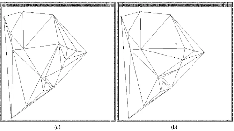
The process of Delaunay triangulation generates rela-tional graphs from the two sets of point-features. An exam-ple is shown in Fig. 1. More formally, the point-sets are the nodes of a data graph GD = {', ED} and a model graph GM =
{0, EM}. Here, EDÕ'¥' and EMÕ0¥0 are the
edge-sets of the data and model graphs. Key to our matching process is the idea of using the edge-structure of Delaunay graphs to constrain the correspondence matches between the two point-sets. This correspondence matching is de-noted by the function f : ' Æ 0 from the nodes of the data-graph to those of the model graph. According to this notation, the statement f(n)(i) = j indicates that there is a match between the node i Œ ' of the model-graph to the node j Œ 0 of the data-graph at iteration n of the algo-rithm. We use the binary indicator or assignment variable
si jn f i j
n
,
0 5
=%&
0 5
0 5
='
10if
otherwise (5) to represent the configuration of correspondence matches.
3.2 Relational Constraints
In performing the matches of the nodes in the data graph GD, we will be interested in exploiting structural constraints provided by the edges of the model graph GM. These con-straints are purely symbolic in nature and are represented by configurations of nodes in the model graph. We use rep-resentational units or subgraphs that consist of neighbor-hoods of nodes that are connected to a center node by arcs to impose consistency constraints. For convenience, we re-fer to these structural subunits or N-ary relations as super-cliques. The superclique centered on the node indexed i in the data graph GD with arc-set ED is denoted by the set of
nodes CiD = »i
<
k i k; ,1 6
ŒEDA
. The matched realization of this superclique is denoted by the relationGi
C
f u f u f u
iD
=
2 7 2 7
1, 2 ,K, .Key to our matching scheme is the idea of computing the probability of the match of the data-graph node i to the model-graph node j. We realize this goal by comparing the configuration of matches residing on the data-graph super-clique CiD with the configuration of nodes that constitute the model-graph superclique centered on the node j, i.e., CjM = jU
=
l j l; ,1 6
ŒEMB
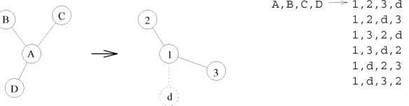
.To realize this comparison we require a dictionary of possible mappings between the nodes of the data-graph clique CiD and those of the model-graph superclique CjM so as to bind matches for the purposes of comparison. If the two supercliques are of the same size, then these so-called structure-preserving mappings are found by permuting the noncenter nodes. However, when the supercliques are of different size, then we must pad the smaller unit with dummy nodes to raise it to the same size as the larger unit. This increases the complexity of the task of dictionary com-pilation. First, we must insert one or more dummy edges into the smaller superclique between each pair of the exist-ing edges. Second, we perform cyclic permutation of each of the resulting padded configurations. This process is il-lustrated in Fig. 2. The process effectively models the dis-ruption of the adjacency structure of the data graph caused by the addition of clutter elements or the loss of elements due to segmental drop-out. Since it is intrinsically symbolic in nature, the resulting dictionary is invariant to scene translations, scalings, or rotations.
To be more formal, the set of feasible mappings, or dic-tionary, for the model-graph superclique CjM is denoted by
Qj = {S}. The individual structure-preserving mappings are sets of Cartesian pairs which associate individual data-graph
[image:4.570.101.477.60.271.2](a) (b)
nodes from the superclique CiD with counterparts in the model-graph superclique CjM. The center nodes are always paired with one another. The neighborhood nodes are paired either with other neighborhood nodes or with dummy nodes. Each dictionary item is a structure-preserving mapping of the form
S=
1 6 1 6 1 6
i j, »J
k l, ; k l, Œ4
CiD-:?
i9
»dummy¥
4
CjM-; @
j9
»dummyL
. (6) It is the size of the dictionary which poses the main computational bottleneck in the application of our ing scheme. For instance, if we are considering the match-ing of supercliques of the same size, i.e., no paddmatch-ing is re-quired, then there are Cj cyclic dictionary items of the su-perclique Cj. If, on the other hand, the cyclicity constraint is lifted, then there are Cj! items. When padding is intro-duced, then the complexity is increased. If the model-graph relation S is being compared with the match residing on the data-graph clique Cj, then there areS
Cj S Cj
--
-1 1
2 7
4
9 4
! !9
! cyclic dictionary items andS C
S C
j j
-1
2 7
4
9
! ! noncyclic dictionary items.
3.3 Structural Matching Probabilities
In this section, we present a simple model which can be used to assign probabilities to putative correspondence matches based on their consistency with the assigned matches on neighboring nodes of the graph. This model draws on a refinement of the relational consistency measure originally reported by Wilson and Hancock [45]. Our goal is to compute the probability of assigning the correspondence match f(n+1)(i) = j to the center node i of the data-graph clique CiD at iteration n + 1. In order to draw on contextual information concerning the consistency of this putative cor-respondence match, we condition the probability on the matches assigned to the neighboring nodes of the clique at iteration n of the algorithm, The relevant set of neighbor-hood matches is denoted by the configuration
$ ;
Gi
0 5
n =J
f0 5
n1 6
l lŒCiD-:?
iL
.In other words, we aim to compute the correspondence matching probability
P f i j P f i j
P
n
i n
n
i n i
n
+
+
=
== 1
1
0 5
0 5
0 5
0 5
0 5
0 5
$4
0 5
4 9
,$9
$G
G G
. (7)
Since the probability of the assigned neighborhood configu-ration P
4 9
G$i0 5
n appearing in the denominator is a fixed property of the data-graph clique CiD at iteration n, we can confine our attention to developing the joint configura-tional probability P f4
0 5
n+10 5
i = j,G$i0 5
n9
appearing in the nu-merator. According to the Bayes formula,P f i j
P f i j
P f i j
n
i n
n
i n n
i n j
+
+
+
Œ
=
== =
Â
1
1 1
0 5
0 5
0 5
0 5
0 5
0 5
0 5
$4
4
0 5
0 5
,$9
9
,$G
G G 0
. (8)
To simplify the development, we use the notation
Gi j, =
J
f0 5
n+10 5
i = j f,0 5
n1 6
l," Œl CiD-:?
iL
to represent the configuration of matched nodes on the superclique CiD with the putative update f(n+1)(i) = j at the center node.As we noted in Section 3.2, the consistent labelings available for gauging the quality of the putative match f(n)(i) = j are represented by the set of relational mappings from the data-graph clique CiD onto the model graph clique centered on the node j, i.e., CjM is encapsulated by the dic-tionary Qj. To evaluate the consistency of the putative con-figuration of matches Gi,j, we use the Bayes rule to expand the probability P(Gi,j) over the structure preserving map-pings between the supercliques CiD and CjM belonging to the dictionary Qj. In other words, we write
P i j P i jS P S
S j
G G
Q
, , .
4 9
=4 9 0 5
Œ
Â
. (9) [image:5.570.139.431.65.141.2]The development of a useful graph-mapping measure from this expression requires models of the processes at play in producing matching errors. These models are repre-sented in terms of the joint conditional matching probabili-ties P
4 9
Gi j, S and of the joint priors P(S) for the consistentrelations in the dictionary. In developing the required mod-els, we will limit our assumptions to the case of matching errors which are memoryless and occur with a uniform probability distribution.
To commence our modeling of the conditional probabili-ties, we assume that the various types of matching error for nodes belonging to the same superclique are memoryless. In direct consequence of this assumption, we may factor-ize the required probability distribution over the symbolic constituents of the relational mapping under considera-tion. As a result, the conditional probabilities P
4 9
Gi j, S may be expressed in terms of a product over label confusion probabilitiesP i jS P f k l
k l S
G, ,
4 9
=1 5
3 8
1 6
Œ
’
. (10) Our next step is to propose a two component model of the processes which give rise to erroneous matches. The first of these processes is initialization error, which we aim to rec-tify by iterative label updates. We assume that initialization errors occur with a uniform and memoryless probability Pe. The second source of error is structural disturbance of the relational graphs caused by noise, clutter or segmentation error. We assume that structural errors can also be modeled by a uniform distribution which occurs with probability Pf.This probability governs the insertion of dummy nodes necessary to make the comparison of differently sized cliques feasible. Dummy nodes are inserted into the smaller clique to raise it to the same size as the larger clique. Under these dual assumptions concerning the nature of matching errors, the confusion probabilities appearing under the product of (10) may be assigned according to the following distribution rule
P f k l
P P f k l
P P f k l l
P k
l
e e
1 6
3 8
=4 92 7 1 6
4 9
1 6
- - =
- π π
=
%
&
KKK
'
KK
K
1 1
1
f f
f
if
if and dummy if = dummy or
dummy
(11)
The three cases under this distribution rule require fur-ther explanation. The first case corresponds to the situation in which there is agreement between the current match and that demanded by the dictionary item S. The second case corresponds to matching disagreements which do not in-volve dummy nodes. The third case arises when the super-cliques under consideration are of different size. If either the data-graph node k or model-graph node l is a dummy node inserted for the purposes of padding, then the null-match probability is assigned.
As a natural consequence of this distribution rule, the joint conditional probability is a function of three physically meaningful variables. The first of these is the Hamming distance H(Gi,j, S) between the assigned matching and the feasible relational mapping S. This quantity counts the number of conflicts between the putative configuration of matches Gi,j assigned to the data-graph superclique CiD and those assignments demanded by the relational mapping S
onto the model-graph superclique CjM. With the binary in-dicator variables used to represent the matching process, the Hamming distance is given by
H i j S sk ln
k l S
G, ,
,
,
4 9
4
0 5
9
1 5
=
-Œ
Â
1 . (12)The second variable is the sum of the number of dummy nodes required for padding. This second quantity is equal to the size difference between data-graph clique CiD and the model-graph clique CjM and is denoted by
Y G
4 9
i j, = CiD - CjM . (13) The final variable is the size of the larger superclique, i.e.,Ri j, =max CiD,CjM . (14) With these ingredients, the resulting expression for the joint conditional probability acquires an exponential character
P
4 9 4 92 7
Gi j, S = 1-Pf 1-Pe Ri j, -H4
Gi j, ,S9 4 9
-Y Gi j, ¥4 9
1-P Pf e H4
Gi j, ,S9
¥ Pf Y G
4 9
i j, . (15) Finally, in order to compute the superclique matching prob-ability P(Gi,j), we require a model of the joint-priors for the dictionary items. Here, we assume that the unit probability mass is uniformly distributed over the relevant items, i.e.,P S
j
0 5
= 1Q . (16)
Collecting together terms in the expression for P(GiΩS) and substituting for the joint priors for the dictionary items, we obtain the following expression for the superclique match-ing probability
P i j Ki j k H S k
j
e i j i j
S j
G
Q Q G Y G
, ,
, ,
exp ,
4 9
=!
-4
4 9
+4 9
9
"$#
Œ
Â
f , (17)where Ki j, =
2 74 9
1-Pe 1-Pf Ri j, . The two exponential con-stants appearing in the above expression are related to the matching-error probability and the null match prob-ability, i.e.,k P
P
e
e e
=ln
2 7
1 -andk P P
P
e
f
f f
=ln
2 74 9
1- 1- .Pe =P = -+
f
20 '
0 ' . (18)
The probability distribution given in (17) may be re-garded as providing a natural way of softening the hard relational constraints operating in the model graph. The most striking and critical feature of the expression for P(Gi,j) is that the consistency of match is gauged by a series of ex-ponentials that are compounded over the dictionary of con-sistently mapped relations.
The key idea underlying our dual-step EM algorithm for recovering transformational geometry is to gate contribu-tions to the expected log-likelihood function using rela-tional constraints. In order to realize this process, we re-quire the expected value of the assignment variables, i.e., E si j
0 5
,n . With the ingredients outlined in this section, the expected assignment variable is equal toE s
P S P S
P S P S
i j n i j n i j S i j S j j j , , , ,
0 5
0 5
4 9 0 5
4 9 0 5
= = Œ
Œ Œ
Â
Â
Â
z G G Q Q 0. (19)
Substituting from (17), we make the role of Hamming dis-tance and the number of padding or dummy nodes more explicit by writing
z f f i j n i j j
e i j i j
S i j j
e i j i j
S j
K
k H S k
K
k H S k
j j , , , , , , , exp , exp ,
0 5
4
4 9
4 9
9
4 9
4 9
4
9
=
- +
!
"$#
- +
!
"$#
Œ Œ Œ
Â
Â
Â
Q G Y G
Q G Y G
Q
Q
0
. (20)
4 T
HEU
NIFIEDM
ATCHINGA
LGORITHMOur aim is to extract geometric transformation parameters and correspondence matches from the two point-sets using the EM algorithm. When couched probabilistically, the goal can be succinctly stated as that of jointly maximizing the data-likelihood p(wΩz, f, F) over the space of correspon-dence matches f and the matrix of transformation parame-ters F. We realize this process using a dual-step or hierar-chical version of the EM algorithm. The utility measure un-derpinning the algorithm is the expected log-likelihood function which allows parameters to be estimated when confronted with incomplete data. The basic idea underlying the algorithm is to iterate between the expectation and maximization steps until convergence is reached. Expecta-tion involves updating the a posteriori probabilities of the missing data using the most recently available parameter estimates. In the maximization phase, the model parame-ters are recomputed to maximize the expected value of the incomplete data likelihood.
According to the original work of Dempster et al. [12] the expected likelihood function is computed by weighting the current log-probability density by the a posteriori measurement probabilities estimated from the preceding maximum likelihood parameters. Here, we wish to exploit Jordan and Jacobs [23] idea of augmenting the maximum
likelihood process with a graphical model. From an archi-tectural standpoint, the graphical model can be regarded as a supervisor network which effectively gates contributions to the expected log-likelihood function. The novelty of the work reported here is to develop a variant of this idea in which it is the bipartite graph, i.e., f, which gates the likeli-hood function for the transformation parameters F. This graph represent the current state of correspondence match between the two point-sets.
We extract both maximum likelihood geometric trans-formation parameters and maximum a posteriori matching probabilities by applying coupled update operations to the gated likelihood function. In this way, the consistency of the structural matching process can guide the pose recovery process. Likewise, error probabilities derived from the po-sition residuals are used to guide the correspondence matching process. When the joint likelihood function is maximized in this way, then the correspondence matches play the role of missing data.
4.1 Mixture Model
Our basic aim is to jointly maximize the data-likelihood p(wΩz, f, F) over the space of correspondence matches f and the matrix of geometric transformation parameters F. We can regard the set of data-graph measurement vectors, i.e.,
w, as the input to our process. The model-graph measure-ments, i.e., z, on the other hand, are the outputs which are to be stochastically recovered from the transformation pa-rameters, i.e., F and the structural state of the bipartite cor-respondence matching graph, i.e., f. For this reason, rather than commencing our discussion from the complete likeli-hood function p(wΩz, f, F), we turn to the incomplete data likelihood, i.e., p(wΩf, F).
Our first model assumption is that the incomplete data-likelihood can be factorized over the set of data-graph measurement vectors. In other words, we assume that the measurement process is conditionally independent given the transformation parameters and the model-graph meas-urements. As a result, we write
p f p w fi
i
w ,F ,F
3
8
=3
8
Œ
’
r'
. (21)
The next step is to account for the missing variables by de-veloping a mixture model over the set of model-graph measurements. Using the Bayes rule, we expand the in-complete data-likelihood over the set of model-graph measurements
p w fi p w z fi j
j
r r r
,F , ,F
3
8
=4
9
Œ
Â
0
. (22)
Our key modeling ingredient is to exploit the binary as-signment variables as exponential indicators in developing a measurement density for the correspondence matches. We take the view that if data graph node i matches to model-graph node j, then it is the measurement density p w z
4
r ri, jF9
p w z fr ri j p w zr ri j si j si j
, ,F , F , ,
4
9 4
=9
r1- . (23) We are now in a position to assemble the expression for the incomplete data-likelihood by substituting (22) and (23) into (21). The result isp f p w zi j s s
j i
i j i j
w , , , ,
F F
3
8
=4
9
-Œ
Œ
Â
’
r r r10 '
. (24)
Our route to maximizing the incomplete data-likelihood is to apply the EM algorithm [12], [23] to the expected log-likelihood function. The idea behind the EM algorithm is to compute the conditional log-likelihood for a new pa-rameter set given the preceding papa-rameter estimates. In the case of our incomplete data-likelihood, the conditional log-likelihood is
Q n n P z w
i
j i n j
F + F F
Œ Œ
0 5 0 5
1 =Â Â
0 5
' 0
r r ,
si j
0 5
,n lnp w zr ri, jF0 5
n+ +4
-si j0 5
,n9
ln!
1"$#
1 r . (25)
To simplify matters, we make a mean-field approximation and replace si j
0 5
n, by its average value, i.e., we make use of the fact that E s4 9
i j0 5
n, =zi j0 5
n, . In this way, the structural matching probabilities gate contributions to the expected likelihood function, i.e.,Q n n P z wj i n
j i
F + F F
Œ Œ
0 5 0 5
1 =Â
Â
r r ,0 5
0 '
zi j
0 5
,nlnp w zr ri, jF0 5
n+ -lnr +lnr!
1"
$#
. (26)
This is an important statement of our matching framework. The first term inside the round-braces is appropriate to pa-rameter estimation, while the second term is appropriate to the computation of correspondence matches. In the case of parameter estimation and as demonstrated by Dempster, et al. [12], maximizing the incomplete expected likelihood function is equivalent to maximizing the following condi-tional likelihood function
Q$ n n P z wj i, n
j i
F + F F
Œ Œ
0 5 0 5
1 =Â
Â
r r0 5
0 '
zi j
0 5
n, lnp w zr ri, jF0 5
n+1. (27) The structure of this component of the expected log-likelihood function requires further comment. The meas-urement densities p w zr ri, jF0 5
n+1 model the distribution of error-residuals between the observed data-point positionr wi and the predicted position of the model point rzj under the current set of transformation parameters F(n+1). The log-likelihood contributions at iteration n + 1 are weighted by the a posteriori measurement probabilities P z wr rj i,F0 5
ncomputed at the previous iteration n of the algorithm. The individual contributions to the expected log-likelihood
function are gated by the structural matching probabilities
z
0 5
i jn, . This chimes with the hierarchical mixture of experts algorithm of Jordan and Jacobs [23], where an expert layer is responsible for gating. However, whereas Jordan and Jacobs gating layer is parametric, ours is structural.We now turn our attention to the recovery of correspon-dence matches. As we mentioned earlier, the component of the expected log-likelihood appropriate to this task is the second term under the round braces of (26). Since the uni-form density r is a constant whose value is less than unity, the goal of correspondence matching is to maximize the quantity
Z P z w
j j i n i j n i =
Œ ŒÂ
Â
0 ' r r,F
0 5 0 5
z , . (28) It is interesting to note that this is just the MAP criterion used by Wilson and Hancock [45] in their work on graph-matching by discrete relaxation.4.2 Expectation
In the expectation step of the EM algorithm, the a posteriori probabilities of the missing data (i.e., the model-graph measurement vectors, zrj) are updated by substituting the revised parameter vector into the conditional measurement distribution. Using the Bayes rule, we can rewrite the a posteriori measurement probabilities in terms of the com-ponents of the corresponding conditional measurement densities
P z w
p w z
p w z
j i
n i j
n i j n j n i j n j
r r r r
r r , , , , F F F + ¢ ¢ ¢Œ
=Â
10 5
0 5
0 5
0 5
0 5
a a
0
. (29)
The mixing proportions are computed by averaging the a posteriori probabilities over the set of data-points, i.e.,
ai jn j i n
i
P z w
, ,
+
Œ
=
Â
1 1
0 5
0 5
' ' r r F . (30)
In order to proceed with the development of a point registration process, we require a model for the conditional measurement densities, i.e., p w z
r ri, jF0 5
n. Here, we assume that the required model can be specified in terms of a mul-tivariate Gaussian distribution. The random variables ap-pearing in these distributions are the error residuals for the position predictions of the jth model point delivered by the current estimated transformation parameters. Accordingly, we writep w z
r ri, jF0 5
n =1 2 1 2 3 2 1 p
0 5
Â4 9
0 5
4 9
0 5
- Â
!
-"
$#
exp ei j, Fn T ei j, Fn . (31) In the above expression, S is the variance-covariance matrix for the vector of error-residuals ei j n
i j
n
w z
,
4 9
F0 5
= -0 5
r r between
and their counterparts in the data, i.e., wri. Formally, the matrix is related to the expectation of the outer-product of the error-residuals i.e., Â =
!
"
$#
Eei j,
4 9 4 9
F0 5
n ei j, F0 5
n T . Accord-ingly, we compute the following estimate of S~ , , , , Â =
- Œ Œ Œ ŒÂ
Â
Â
Â
P z w w z w z
P z w
j i n j i i j n i j n i j n T j i n j i i j n
r r r r r r
r r
F
F
0 5 0 5
0 5
0 5
0 5 0 5
4
94
9
0 ' 0 ' z z
. (32)
4.3 Maximization
As pointed out earlier, the maximization step of our unified or synergistic matching algorithm is based on dual coupled update processes. The first of these aims to locate maxi-mum a posteriori probability correspondence matches. The second update operation is concerned with locating maxi-mum likelihood transformation parameters. We effect the coupling by allowing information flow between the two processes. In the remainder of this section, we detail the maximization steps used to realize this coupling.
4.3.1 Maximum a posteriori Probability Matches
Point correspondences are sought so as to maximize the a posteriori probability of structural match. The updated con-figuration of correspondence matches is located by maxi-mizing the second component of the expected log-likelihood function defined in (26). The resulting update formula is
fn i P z w
j j i
n i j n + Π+ =
1 10 5
0 5
arg max ,0 5 0 5
,
0
r r F z . (33) Once this update equation has been applied, the un-matched model-graph nodes are identified for removal from the triangulation. At this point, the edited set of model feature-points is retriangulated to correct potential struc-tural errors. We provide more details of this graph-editing process in the next subsection. The structural matching probabilities z
0 5
i jn,+1 are also updated using (20) as outlined in Section 3.4.3.2 Updating the Triangulation
In order to overcome this source of potential structural corruption, at the end of each iteration we retriangulate the graph in order to accurately reflect the structure of the points under the current estimate of the transformation parameters. We have recently shown how this process of active graph reconfiguration or editing can be realized as a MAP estimation process [44]. However, rather than con-fining itself purely to node relabeling, the algorithm now encompasses the possibility of node insertions or dele-tions together with the implied modification of the Delau-nay edge-set. This process is illustrated in Fig. 1. Details of the derivation are outside the scope of this paper. The ba-sic idea is to gauge the net effect of deleting a node by examining those contributions to the consistency measure that arise from modification of the supercliques containing the node in question. This set is constructed by identifying those nodes that form a superclique with node i in graph
GD, i.e., Ci i D-
:?
, and determining the new superclique set for these nodes in the reconfigured graph GD¢. We let ci+
denote the superclique set of object i in graph GD and ci
-denote the corresponding superclique set in the reconfig-ured graph G¢M. With this notation, the change in the MAP criterion of (28) caused by the deletion of the node i is proportional to
D
Q Q G
i
i j j l
e l j S
P K k H S
i j -ΠΠ=
-Â
Â
f c , ,exp
4 9
, . (34) By contrast, when considering the change in the MAP criterion caused by reinsertion of the node i, it is the super-clique set ci+ to which we turn our attention. The corre-sponding change to the MAP criterion is proportional toD F
Q Q G
i f i i
n i j
j l
e l j S
P z w K k H S
i j + ΠΠ=
-+Â
Â
r r0 5
,0 5
, exp4 9
, ,c
. (35) The decision criteria for node deletion or reinsertion are as follows. We delete node i provided D+i <D-i and reinstate it provided D+i >D-i. In addition to this structural modifica-tion, we can improve the robustness of parameter estima-tion by removing points in the model-set which have no correspondence in the data-set when computing the ex-pected log-likelihood function in the expectation step of the EM algorithm. Once these points are removed, we must once again retriangulate the point set in order to reflect the change in structure. At each iteration of the maximization stage, we also try reintroducing any deleted points back into the data set.
4.3.3 Maximum Likelihood Parameters
With the Gaussian measurement process described in Section 4.2, the maximization step of the EM algorithm simply reduces to computing the weighted squared error criterion
Q¢
F0 5 0 5
n+1 Fn =-
ÂŒ Œ
+ - +
Â
Â
P z wj i nj i i j n i j n T i j n r r
,F
0 5 0 5
, ,4 9
F0 5
,4 9
F0 5
0 '
z e 1 1e 1 . (36)
In other words, the a posteriori probabilities P z w
r rj i,F0 5
n and the structural matching probabilities zi j0 5
n,effectively regulate the contributions to a weighted squared-error criterion. In the remainder of this subsection, we provide details of how maximization is realized for the two different geometries described in Section 2.
• Affine Geometry: In the case of affine geometry, the transformation is linear in the parameters. This allows us to locate the maximum-likelihood parameters di-rectly by solving the following system of saddle-point equations for the independent affine parameters fk l
0 5
n,+1∂ ¢
∂ =
+
+
Q n n
k l n
F 1 F
1 0
0 5 0 5
0 5
f , . (37)
For the affine transformation the set of saddle-point equations is linear and are, hence, easily solved by us-ing matrix inversion. It is straightforward to show that the updated matrix of affine parameters must satisfy the following implied system of linear equations
P z wj i n
j i
i j n
r r
,F
0 5 0 5
, ¥ Œ ŒÂ
Â
0 ' zr r r
wi- n zj TÂ z Uj
!
4
F0 5
+19
-1"
$#
=0, (38) where the elements of the matrix U are the partial de-rivatives of the affine transformation matrix with re-spect to the individual parameters, i.e.,U =
1 1 11 1 10 0 0 . (39) As a result, the updated solution matrix is given by
Fn j i Fn
j i i j n j T j T
P z w z U z
+
Œ Œ
-=
Â!
Â
Â
"
$
##
1 1
1
0 5
r r0 5 0 5
r r, ,
0 '
z
¥
Â!
Œ Œ
"
$
##
-Â
Â
P z wj i n w U zj i i j n i T j T
r r , r r
, F
0 5 0 5
0 '
z 1 . (40)
This allows us to recover a set of improved transfor-mation parameters at iteration n + 1. Once these are computed, the a posteriori measurement probabilities may be updated by applying the Bayes formula to the measurement density function. The update procedure involves substituting the parameter matrix of (1) into the Gaussian density of (31) and applying the Bayes theorem.
• Perspective Geometry: In the case of perspective geome-try where we have used homogeneous coordinates, the saddle-point equations are no longer soluble in a closed-form linear fashion. The maximum likelihood transformation parameters satisfy the condition
F F F n j i n j i
P z w
+
Œ Œ
=
Â
Â
1
0 5
arg min r r ,0 5
0 '
z
0 5
i j,n4
wri-zrj0 5
n+19 4
TÂ-1wri-zr0 5
jn+19
. (41) Following Horaud et al. [20], we solve this maximi-zation problem using the Levenberg-Marquardt tech-nique. This is a nonlinear optimization technique that offers a compromise between the steepest gradient and inverse Hessian methods. The former is used when close to the optimum while the latter is used far from it. In other words, when close to the optimum, parameter updating takes place with step-size pro-portional to the gradient —FQ¢ F F0 5
n . When far from the optimum, the optimization procedure uses second-order information residing in the Hessian, H,of Q¢ F F
0 5
n ; the corresponding step-size for the pa-rameter matrix F is H-1—FQ F F0 5
n . Central to the Levenberg-Marquardt method is the idea of exerting control over these two update modes using a positive parameter l. This parameter defines the elements of the matrix LLk l, =
%&'
1+ k=l1
l if
otherwise (42) According to the Levenberg-Marquardt method, the step-size dfl for the parameter fl is found by solving the following set of linear equations
L
F F F F
k l n k l l l n k Q Q , ∂ ¢ ∂ ∂ = ∂ ¢ ∂ =
Â
2 13
0 5
0 5
f f df f . (43)
The parameter l is chosen to be large if the log-likelihood increases when an optimization step is taken; in this case, the optimization process operates in steepest gradient mode. If, on the other hand, the expected likelihood decreases, then l is reduced to-wards zero; in this case, the optimization process op-erates in inverse Hessian mode. When controlled ef-fectively, this method is less prone to local conver-gence than the standard steepest gradient descent method, while offering efficiency gains over the in-verse Hessian method. In fact, we find the Levenberg-Marquardt optimization converges in 5-10 iterations. Steepest-gradient takes up to 10 times longer to con-verge. Although our research-code is not optimized for efficient execution, typical registration experi-ments involving up to 100 points take tens of seconds on an SGI RS5000 workstation.
Before proceeding, it is important to offer a word of caution and to stress that degeneracies may be encountered in the estimation process if we confront affine data with a per-spective model. We have not investigated this pathological case in our experiments.
Our final comment on the implementation concerns the execution speed of the algorithms. The main computational bottleneck is the evaluation of the structural matching probabilities. As outlined in Section 3.2, here, the main source of complexity is the size of the dictionary. Compared with this, the computation of transformation parameters represents a relatively small overhead. In the case of affine geometry, the recovery process can be realized rapidly us-ing efficient matrix inversion. In the perspective case, pa-rameter recovery is slower since iterative numerical optimi-zation is needed. However, it must be stressed that we have not investigated the use of efficient search algorithms here because of the bottleneck associated with the dictionary prior. As a concrete example, when run on a SGI RS5000 processor, our registration method takes tens of minutes.
5 E
XPERIMENTALR
ESULTStwo distinct strands. First, we will provide an algorithm sen-sitivity analysis. Here, we confine ourselves to the affine variant of the matching process. The aim is to experimentally compare our dual-step algorithm with the performance of each of its components taken individually. In other words, we provide comparison with maximum a posteriori probability correspondence matching and least squares parameter re-covery. These two comparisons serve to demonstrate that the combined modeling of both point correspondences and transformation geometry yields significant advantages in terms of accuracy of convergence over their individual use.
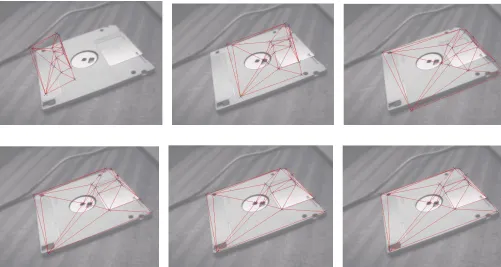
In the second strand of our experimental investigation, we will furnish examples demonstrating the use of the dual-step matching scheme on real world imagery. Here, we will use two different data sets. The first of these in-volves perspective views of 3.5-inch floppy discs. The sec-ond example involves matching distorted aerial image data against a digital map.
5.1 Algorithm Comparison
The aim of this section is to demonstrate how the dual-step matching algorithm performs in comparison with the repeated iteration of its individual component parts. In this part of our study, we confine our attention to the matching of synthetic point-sets under affine geometry. The two algorithms used for comparison are
• Maximum a posteriori probability correspondence matching: In this set of experiments, we aim to dem-onstrate how our dual-step EM method performs in comparison with MAP correspondence matching us-ing structural constraints [45]. The update process is realized by keeping the parameter matrix static at the value F(0) and iteratively updating the discrete corre-spondence assignments. The update rule for the cor-respondence matches is
f n i P z w
j j i i j
n
+
Œ
=
1 0
0 5
0 5
arg max ,0 5 0 5
,0
r r F z
. (44) This aspect of our study aims to investigate the role played by the explicit modeling of the transforma-tional geometry.
• Maximum Likelihood Registration: Here, we focus on the iterative estimation of affine registration pa-rameters by applying the standard EM algorithm to the ungated log-likelihood function. This corresponds to clamping the structural gating probabilities with a uniform and static distribution over the complete space of possible correspondences during the itera-tion of the parameter estimaitera-tion process. The update equation for the affine parameter matrix is
Fn j i Fn
j i
j T
j T
P z w z U z
+
Œ Œ
-=
Â!
Â
Â
"
$
##
1 1
1
0 5
r r0 5
r r,
0 '
¥
Â!
Œ Œ
"
$
##
-Â
Â
P z wj i n w U zj i
i T
j T
r r ,F
0 5
r r0 '
1
. (45)
The aim here is to investigate the effect of structural gating on the estimation of transformation parameters.
The results of the comparative study have been obtained using random point sets. This allows us to compare algo-rithm sensitivity in a controlled manner under varying noise conditions. This experimental methodology also al-lows the results to be averaged over a large number of ran-dom experiments and meaningful error bars to be derived from the population statistics. Each of our reported data-points is averaged over 100 random experiments. The error-bars are the standard errors over the set of trials.
5.1.1 Comparison With Standard Structural Matching
In order to demonstrate the relative stability of the dual-step matching scheme under initial parameter choice, we will compare it with a structural graph matching scheme. The algorithm used in this comparison is essentially the discrete relaxation process of Wilson and Hancock [45]. This structural matching technique results solely from the itera-tion of the MAP update process defined in (34), leaving the parameter estimates static. The aim of our study is to dem-onstrate the sensitivity of our method to initial differences in isotropic image scale and overall point-set orientation. The study is based on random dot patterns in which the ground-truth transformational geometry is known.
In Figs. 3a and 3b, we respectively show the final frac-tion of points in correct correspondence as a funcfrac-tion of the initial difference in orientation and scale. The dotted lines show the sensitivity of the standard structural matching scheme, while the solid lines are for the dual-step matching method. It is clear that our dual-step expectation-maximization approach consistently outperforms the stan-dard relational matching scheme. In particular, the range of both rotation and scale over which the dual-step EM scheme successfully recovers meaningful results is signifi-cantly greater than that for the purely structural scheme. For instance, our dual-step method copes well with angle differences of up to 35 degrees, whereas the structural method must be initialized to within 10 degrees. In the case of the scale difference, the dual-step method copes with differences in the range 0.7 to 1.6, whereas the MAP scheme only functions effectively over the range 0.9 to 1.1. How-ever, it must be stressed that the structural method could be rendered considerably more robust if affine invariant measures are used to compute the initial a posteriori matching probabilities.
5.1.2 Comparison With Least Squares Fitting Algorithms
portion of the data-graph and the model. If n• is the final iteration number for the matching algorithm, then the measure of registration accuracy is
A
T wi zj
n i j T
= - •
Œ
Â
1 r r
2 7
1 6
,. (46)
It is important to stress that this figure of merit includes only unmodified points from the original model graphs. In other words, we exclude nodes deleted from the graphs in the re-triangulation step.
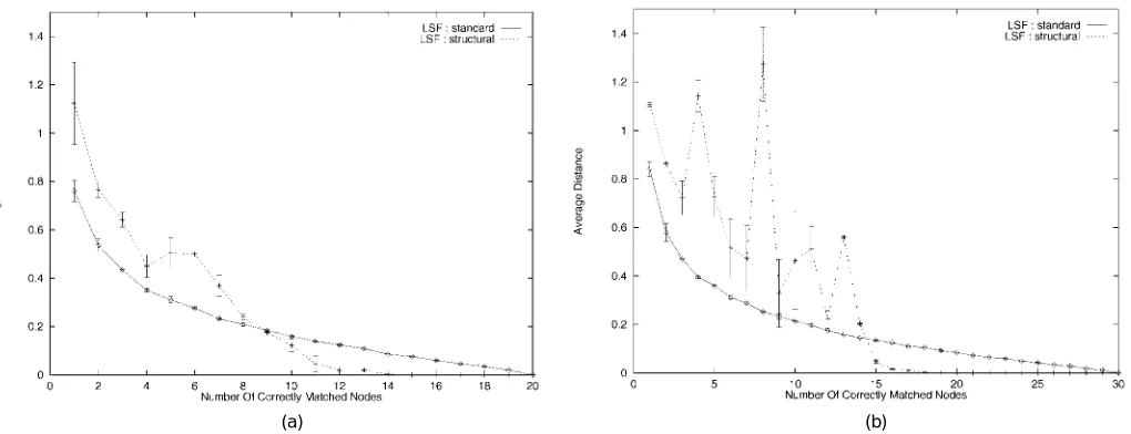
Fig. 4a shows a comparison of the new matching scheme (dashed curve) and the ungated maximum likelihood method (solid curve) of affine parameter estimation. Here, the size of original point-set is 20. Fig. 4b repeats this ex-periment when the size of the point-set is 30. The plots show the average registered point-distance as a function of the fraction of correct correspondence matches.
The main feature to note from these plots is that, pro-vided sufficient correspondences are available, then the
dual-step method outperforms the least-squares method in terms of the registration error. Moreover, provided that the degree of structural error is less than 50 percent, then the average registration error for the dual-step method is con-siderably smaller than for the conventional EM registration method. In fact, when this is the case, then an average point error of less than 0.01 is achievable.
This limiting degree of structural corruption deserves further comment. In Fig. 5, we show a plot of the fraction of supercliques containing a structural error as a function of the fraction of added noise points for the Delaunay graph. From this plot, it is clear that when the fraction of corrupt nodes is 50 percent, then 70 percent of the supercliques contain at least one corrupt edge. In other words, our dual-step EM approach outperforms its conventional counter-part provided that more than 30 percent of the structure of the Delaunay graph remains is intact. Although our matching method is dependent on structural information, it can tolerate a significant degree of structural corruption.
[image:12.570.39.543.60.253.2](a) (b)
Fig. 3. Sensitivity study: The two plots show how the dual-step EM algorithm (solid curve) outperforms MAP-matching (dashed curve) in terms of the fraction of correct correspondence matches. (a) Affine rotation. (b) Affine scaling.
(a) (b)
[image:12.570.37.547.296.492.2]5.2 Real World Imagery
In order to demonstrate the effectiveness of the new matching process on real world imagery, we will consider the following two data-sets:
• Disk Set: This data set consists of a set of digital photographs of 3.5-inch floppy disks. This data-set was chosen since it allows for controlled shifts in viewpoint to be made. The images under investiga-tion include both small viewpoint shifts that are nearly affine, and very large shifts where the con-trolled introduction of strong perspective foreshort-ening will be investigated.
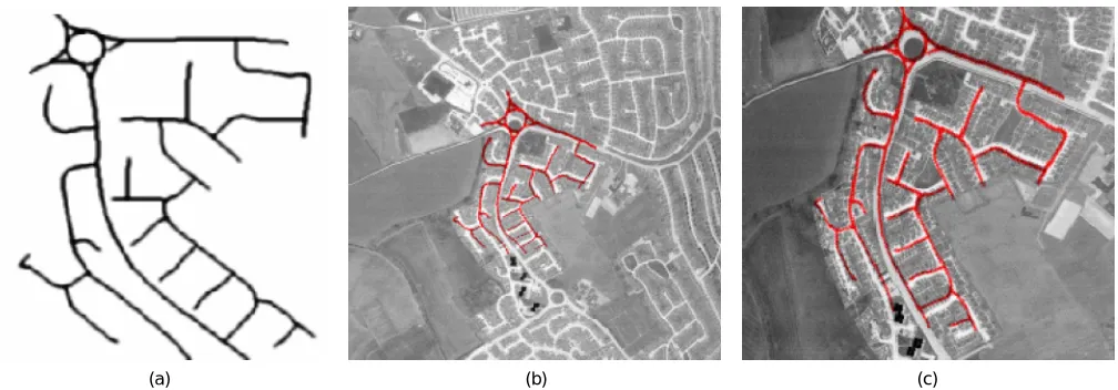
• Road Network: In this experiment, we are concerned with the registration of aerial infrared images against a digital map. The images were taken at nighttime. Under these imaging conditions, the most prominent features are those that radiate absorbed heat. In the urban scenes under study, these features are the tar-mac roads. We therefore chose the road networks as the basis for our graph structures. The nodes in our Delaunay graphs are junctions detected in the road network. It is important to note that these images are distorted due to the geometry of the line-scan proc-ess. The images are captured using horizontal line-scan as the aircraft moves in the vertical direction. The line-scan process is controlled by the rotation of a mirror. For this reason, the images are subject to barrel distortion in the horizontal-direction. In the vertical-direction, there are also sampling irregulari-ties due to the aircraft changing heading due to banking or turbulence.
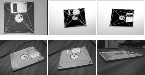
[image:13.570.26.277.60.243.2]We will first consider the task of recognizing planar objects in different 3D poses, which is posed by the set of images of floppy disks. The object used in this study is placed on a desktop. The different object viewing angles are contrived so as to introduce increasing degrees of per-spective foreshortening. The feature points used to trian-gulate the object are corners which are extracted by hand. Fig. 6 shows a sequence of object-views with the triangu-lations of the hand segmented feature-points superim-posed. The first oblique view in the sequence is taken as the object-model; the remaining object-poses are used to test the matching process.
Fig. 5. Effect of adding controlled fractions of relational clutter to De-launay graphs.
[image:13.570.30.539.459.725.2]
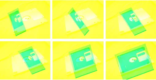
Fig. 7 shows the initial and final poses for the registra-tion of various images in the dataset. In each case, the fraction of correct initial correspondences was
approxi-mately 50 percent. From the superimposed images, it is clear that the recovered final poses are accurate.
[image:14.570.127.449.59.676.2]
(a) (b)