Linear robust H-infinity stochastic control theory on the insurance premium-reserve processes

(1)

Linear Robust

H

∞

Stochastic Control Theory on the

Insurance Premium-Reserve Processes

Thesis submitted in accordance with the requirements of

the University of Liverpool for the degree of Doctor in Philosophy

by

Lin Yang

(2)

Abstract

This thesis deals with the stability analysis of linear discrete-time premium-reserve (P-R) systems in a stochastic framework. Such systems are characterised by a mixture of the premium pricing process and the medium- and long- term stability in the ac-cumulated reserve (surplus) policy, and they play a key role in the modern actuarial literature. Although the mathematical and practical analysis of P-R systems is well studied and motivated, their stability properties have not been studied thoughtfully and they are restricted in a deterministic framework.

In Engineering, during the last three decades, many useful techniques are developed in linear robust control theory. This thesis is the first attempt to use some useful tools from linear robust control theory in order to analyze the stability of these classical insurance systems.

Analytically, in this thesis, P-R systems are first formulated with structural prop-erties such that time-varying delays, random disturbance and parameter uncertain-ties. Then as an extension of the previous literature, the results of stabilization and the robust H∞-control of P-R systems are modelled in stochastic framework. Mean-while, the risky investment impact on the P-R system stability condition is shown. In this approach, the potential effects from changes in insurer’s investment strategy is discussed. Next we develop regime switching P-R systems to describe the abrupt structural changes in the economic fundamentals as well as the periodic switches in the parameters. The results for the regime switching P-R system are illustrated by means of two different approaches: markovian and arbitrary regime switching systems. Finally, we show how robust guaranteed cost control could be implemented to solve an optimal insurance problem.

(3)

List of Figures

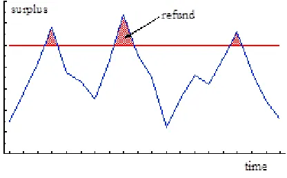
2.1 De Finetti’s approach to control of surplus. . . 12

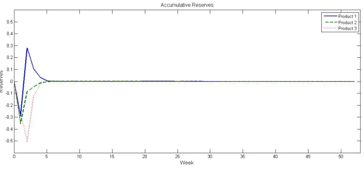
3.1 The movement of the accumulated reserve for each dependent product. . 39

3.2 The premium process for each dependent product. . . 39

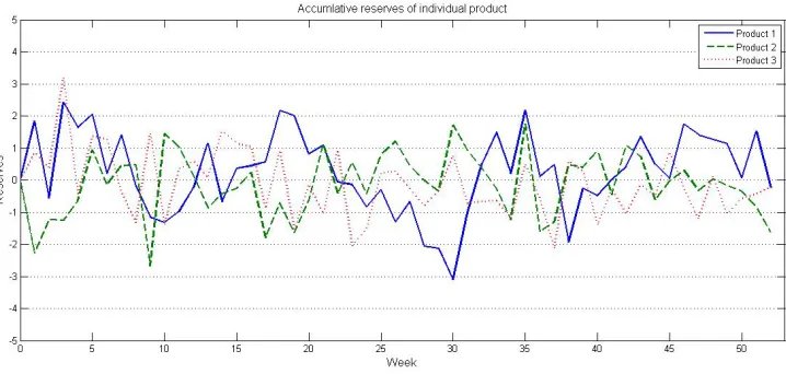
3.3 The movement of the accumulated reserve for each dependent product. . 47

3.4 The premium process for each dependent product. . . 47

3.5 The movement of the accumulated reserve for the whole portfolio. . . . 48

4.1 The premium for the three products for the case 6: (m1= 50%, m2 = 50%). 62 4.2 The accumulated reserve for the three products for the case 6: (m1 = 50%, m2= 50%). . . 62

4.3 The premium for the product 2 for the case 1: (m1 = 100%, m2 = 0%), 6: (m1= 50%, m2 = 50%) and 11: (m1= 0%, m2 = 100%). . . 62

4.4 The accumulated reserve for the product 2 for the case 1: (m1 = 100%, m2= 0%), 6: (m1 = 50%, m2 = 50%) and 11: (m1 = 0%, m2 = 100%). . . 63

4.5 The total premium for the case 1: (m1 = 100%, m2 = 0%), 6: (m1 = 50%, m2= 50%) and 11: (m1 = 0%, m2 = 100%). . . 63

4.6 The total reserve for the case 1: (m1 = 100%, m2 = 0%), 6: (m1 = 50%, m2= 50%) and 11: (m1 = 0%, m2 = 100%). . . 64

4.7 Disturbance level wt for the product 2 for all the cases: from t = 0 to t= 52. . . 64

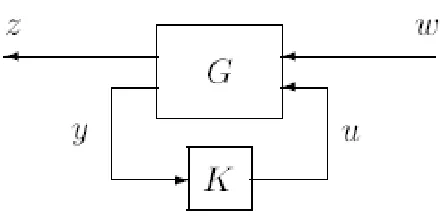
5.1 Feedback Control System . . . 73

5.2 Markovian switching signal: Type 1 . . . 92

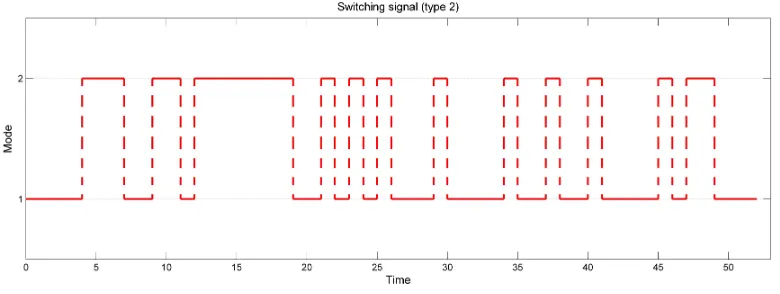
5.3 Markovian switching signal: Type 2 . . . 92

5.4 The evolution of the three Premiums under the Type 1 signal . . . 92

5.5 The evolution of the three Premiums under the Type 2 signal . . . 93

5.6 The evolution of the accumulated reserves under the Type 1 signal . . . 93

5.7 The evolution of the accumulated reserves under the Type 2 signal . . . 94

5.8 The comparison of the total reserve: Type 1 vs Type 2 switching . . . . 94

(7)

6.2 The evolution of the three Premiums under the arbitrary switching signal108 6.3 The evolution of the the three accumulated reserves account under the

(8)

List of publication and

presentation

Publication

1. Yang, L., Pantelous, A.A. and Assa, H. (2015), Robust stability, stabilization and H-infinity control for premium-reserves models in a Markovian regime switching discrete-time framework. ASTIN Bulletin (under revision).

2. Pantelous, A.A and Yang, L. (2015), Robust H-infinity control for a premium pricing model with a pre-defined portfolio strategy. ASCE-ASME Journal of Risk and Uncertainty in Engineering Systems, Part B. Mechanical Engineering, Vol 1, No. 2, pp. 021006: 1-8.

3. Pantelous, A.A and Yang, L. (2014), Robust LMI stability, stabilization andH∞ control for premium pricing models with uncertainties into a stochastic discrete-time framework. Insurance: Mathematics and Economics Vol. 59. pp. 133-143. 4. Pantelous, A.A and Yang, L. (2014), Robust LMI Stability of a Premium Pricing

Model into a Discrete-Time Stochastic Framework. Vulnerability, Uncertainty, and Risk: pp. 1057-1066.

Conference presentation

1. Presentation title: Robust stability, stabilization and H∞ control for premium-reserves models in a Markovian regime switching discrete-time framework. 19th International Congress on Insurance: Mathematics and Economics (IME), 24-26 June 2015, Liverpool UK.

2. Presentation title: Robust stability, stabilization and H∞ control for premium-reserves models in a Markovian regime switching discrete-time framework. 1st Symposium on Quantitative Finance and Risk Analysis (QFRA 2015), 11-12 June 2015, Santorini Greece.

(9)

4. Presentation title: Robust stability of a non-life insurance premium pricing model into stochastic framework. International Conference on Applied Mathematical Optimization and Modelling 2014, 9-11 April, 2014, University of Warwick, UK.

5. Presentation title: On the robust LMI stability of pricing models for non-life in-surance products. Perspectives on Actuarial Risks in Talks of Young Researchers (PARTY) 2013, 27th January -1st February 2013, Switzerland.

(10)

Acknowledgement

It would not have been possible to produce this thesis without a lot of help from many people and it is a great pleasure to have the opportunity to express my gratitude.

First of all and most importantly I would like to express my deepest gratitude to Dr. Athanasios A Pantelous who is a great supervisor to me and also a dear friend. His generous assistance, enthusiastic encouragement and inspiration have always been a continuous support throughout the past four years. I am also indebted to him for cre-ating numerous opportunities for me to learn and grow as a researcher. It’s grateful for me to have numerous insightful discussions, patient help and many conversations from Dr. Athanasios A Pantelous which helped me to clear up several points of confusion.

Many thanks also to Dr. Hirbod Assa for the many discussions and fruitful coop-eration that also led to some of the results in this thesis. I am also grateful to Dr. Jukka Rantala (Managing Director of the Finnish Centre for Pensions, Finland) who has afforded me considerable assistance in enhancing the Chapter 5 both the quality of the findings and the clarity of their presentation.

I would like to thank the University of Liverpool provide me the Graduate Teaching Assistant studentship to support my PhD study.

I also feel grateful to have had the opportunity to be part of the Department of Mathematical science and Institute for Actuarial and Financial Mathematics which created many occasions to interact and benefit from the experience of international researchers.

(11)

Chapter 1

Introduction

1.1 Research problem and Motivation

The premium pricing process, the medium- and long- term stability in the reserve policy under uncertainty are very challenging issues in the insurance world and particularly for

the pricing of General (Non-Life) Insurance products. Additionally, under the Solvency II framework and different other national regulations, the stability and robustness of

the model are parameters that have to be also considered very seriously and thought-fully. Thus, in the insurance market in order for the actuary to be able to price the

gross premium (or market premium) accurately, s/he should have a very good feeling about the financial environment where the various uncertainties are appearing in, the

constraints that the insurance organization is facing from, and the stochastic nature of many other financial and social variables that can interfere in the model. Ideally, even

the delays in reporting the claims and collecting the appropriate information from the client (or/and for the accident or/and event) have to be estimated in order the model

to be more pragmatic and eventually realistic. Thus, the modelling of the uncertain pa-rameters turns up to be one the most essential ones that has to be considered properly

in the development of any effective premium model and reserve process.

Consequently, the premium-reserve (P-R) model has to consider different types of

uncertainties as well as to face the impact of the external disturbances. So far, these parameters have not been implemented altogether in P-R modelling. Therefore, in this

(12)

bringing in the actuarial science some very fruitful ideas and tools from engineering into

a stochastic, discrete-time framework. Here, we are interested not only in examining the stability of the premium process, but also to find a premium such that the stabilization

of the process does occur. In more details, the purpose of the robust stabilization is the design of a state feedback controller such as the resulting closed-loop system is

robust stochastically stable for all admissible uncertainties. Meanwhile this thesis is to investigate several aspects of the problem of stability and stabilization for this premium pricing and accumulated reserve problem subject to markovian and arbitrary switching

regimes.

1.2 Main objectives and contributions

• In Chapter 3, we discuss stability conditions for P-R systems with time-varying delays and outside disturbances in a stochastic framework. This work extends

significantly the recent results proposed by Pantelous and Papageorgiou (2013) [51] in a deterministic framework.

• In Chapter 4, we derive robust H∞ stabilization criteria of the P-R system by considering available risky investments. Here, we discuss the impact of the risky investment on the robustH∞ stabilization performance.

• In Chapter 5, a linear Markovian regime switching system in discrete-time is used to model the medium- and long- term reserves and the premiums (P-R system)

of an insurer. We derive sufficient conditions for stability, the stabilization and the robustH∞-control of a P-R system and analyse the potential effects from the abrupt structural changes in the economic fundamentals as well as the insurer’s strategy over a finite time period.

• In Chapter 6, we derive the result of extended stability andH∞controller design for arbitrary regime switching P-R systems.

(13)

1.3 Structure of thesis

Chapter 2 introduces the reader some important relevant concepts from robust control theory. Then, the history of applying control theory is reviewed with emphasis placed

on some previous results in actuarial literature, which are essential for the generation of the models in this thesis.

Chapter 3 focuses on extending this classic actuarial problem in stochastic frame-work. The main goal of the developments in this chapter is to provide a sufficient condition on the design of a state feedback controller such that proposed closed-loop

P-R system is robust stochastically stable with parameter uncertainties and random disturbances. First, some assumptions are discussed and most of these assumptions

remain same in all the chapters. Then the basic P-R system is introduced and the robust stability and H∞ stability for the system is derived. Numerical examples are used to show the usefulness of the theorems.

Before introducing the regime-switching models in Chapter 5 and 6, Chapter 4

contains the research of P-R system with predefined risky investment. The results derived in Chapter 3 are extended in Chapter 4 in order to characterize robust H∞ stability in the discrete-time linear stochastic P-R system with risky investment.

In Chapter 5, the markovian regime switching model is then introduced in great

de-tails. The fundamental ideas and the mathematical derivation of the regime-switching P-R system are declared, and the robust LMI stability, stabilization and H∞ control problem are discussed. We show that in the case of discrete-time markovian switching linear P-R system there is way to analyse stability and generate a feasible controller.

Chapter 6 focuses on the research on the same problem under arbitrary switching framework. Both Chapter 5 and 6 deal with the problem of the stability analysis of

switched linear P-R systems. Chapter 5 and 6 contain illustrative examples based on the solutions of sufficient LMI conditions.

Before concluding, Chapter 7 introduces a guaranteed cost control approach to determine the optimal feedback controller when multiple performance targets of the

P-R model are required. In short, by a convex optimization problem based on LMI criteria we understand the problem of minimization of a cost function along the stabilization

(14)

contribution of this thesis and point some feasible further research directions for the

topic in this thesis.

1.4 Notation

Throughout this thesis, the matrices are assumed to have compatible dimensions. The

(15)

Chapter 2

Literature Review

2.1 Control Theory: A useful tool in Engineering

Let’s consider a dynamic system; for example a flying aeroplane. The system is in a certain state which is changing all the time. In the case of an aeroplane the state is

described by coordinates of the position of the aeroplane. The changes are caused by internal dynamics of the system and maybe by some outside impulses. The motion

of an aeroplane is governed by the laws of kinetics together with disturbances caused e.g. by changes in wind speed or air pressure. The system should be steered towards a

certain target. Then, we have an observation which gives some information about the present state of the system. The observation may give complete information about the

state, but it may also be disturbed, delayed or otherwise incomplete. Finally, we have some tools or variables which you can control and which affect the state of the system.

In an aeroplane that means different piloting measures.

Thus, the challenge which is considered in control theory is to find a rule which

best satisfies the criteria chosen. These criteria often suggest that the system should not deviate too much from the target and that the correcting measures cannot be too

harsh. In order to do that we must first analyse the statistical properties of the system and build a suitable model for it.

2.1.1 Stability of discrete time delay system

It’s easy to notice that time delay exists in various system such as biological, ecological,

(16)

are often used to model systems, where procession and transmission of information or

material are involved. For example, in economics, the central bank in a country often attempts to influence the economy by adjusting interest rates; the effect of a change in

interest rates takes months to be translated into an impact on the economy. It would be much more complicated to manage and control a system with time delays (especially,

the system with long delay). It has been shown that time delay is often a source of the generation of oscillation and a source of instability of control systems (Kolmanovskii and Myshkis, 1992 [38]).

Usually, stability conditions for time-delay systems can be classified in two types: delay-dependent and delay-independent stability conditions; the former includes the

information on the size of the delay, while the latter does not. Generally speaking, delay independent stability conditions are simpler to apply, while delay-dependent stability

conditions are less conservative especially in the case when the time delay is small. Since delay-dependent stability conditions takes into account impact of the upper bound of

time delay, which makes the stability condition more relevant. In this thesis, our research is mainly based on delay-dependent stability conditions since the time delay

in insurance system is relatively small.

The errors for the system will start to change only after the inherent delay times.

Therefore, it is crucial to properly anticipate and understand the existence of delays and not to over-react. Otherwise, the system is very likely to become much more unstable.

At beginning, much attention is being paid to the delay-dependent stability, stabi-lization, and H∞ control of linear systems with state delays. Less attention has been paid to discrete-time systems with a time-delay, because a linear discrete-time sys-tem with a constant integer time-delay can be transformed into a delay-free syssys-tem by

means of a state-augmentation approach (Mahmoud, 1995 [42]). However this approach is not suitable for systems with either unknown or time-varying delays. Over the past

decades, several articles have appeared on this topic. For example, for small time-varying delays, the descriptor model transformation approach was employed to study

the delay dependent guaranteed-cost control of uncertain discrete-time delay systems; Chen et al. (2003) [17], Bauer et al.(1993) [4], Kim (2001) [37] and Song and Kim(1998)

[64].

In fact, voluminous researches have been done on time-delay systems. A great

(17)

been reported in the literature (see e.g. Chen and Latchman, 1995 [16]; Chu, 1997

[19]; Hui and Hu, 1997 [36]; Dugard and Verriest, 1998 [23]; Su and Chu, 1999 [65]; Hmamed, 2000 [32]; Shi et al., 2000 [61]; Niculescu, 2001 [49]; Boukas and Liu, 2001

[9]; Boukas and Liu, 2002 [10]; Fridman and Shaked, 2002 [26]; Xu et al., 2002 [74]; Xu et al., 2004 [75]; Zhou and Li, 2005 [80]; Chen et al., 2006 [15]; Shu et al., 2006 [63];

Sun et al., 2007 [67]).

Different theorems for delay-dependent stability analysis have been presented in those papers. Meanwhile, many methods have been provided for delay dependent

stability for a class of linear discrete-time systems with time-varying delays. Most importantly, appropriate Lyapunov functionals have been constructed to exhibit the

delay-dependent systems in those literatures, which provide us fruitful techniques to analyse the problems.

2.1.2 Robustness and robust control

Robust control is a branch of control theory whose approach to controller design explic-itly deals with uncertainty. Robust control methods concern a system with admissible

uncertain parameters and/or disturbances. Robustness means the systems achieve ro-bust performance and/or stability in the presence of bounded modelling errors.

Infor-mally, we call a controller designed to be robust when it would work well for a particular set of parameter uncertainties.

2.1.3 H∞ control

Definition 2.1. (Infinity norm)(Zhou et al. 1995 [79])

Let V be a vector space overR and letk · k be a norm defined onV. Then V is a normed space. Now let’s consider aCauchy sequence xt in aBanach space VB. Then

the corresponding infinity norm is defined as

kxk∞,sup{|xt|:t∈N}.

(18)

unexpected disturbances enter the system, this method guarantees that the system will

not greatly deviate from expected trajectories. H∞ control is a key approach to deal with robustness (Green and Limebeer, 1995 [29]). The standard H∞ control problem for delay-free systems was solved in the late 1980s (Zhong, 2006 [78]). Since then, the robust control of time-delay systems has attracted many researchers.

The so-called H∞ norm (see for instance, Francis and Khargonekar, 1995 [24] or Helton and Merino, 1998 [33]), loosely speaking, focuses on the worst possible case and it tries to minimise the maximum of a (linear) loss function of the state and control

variables, for an arbitrary input. In other words, this rule attempts to minimize the loss in system when the circumstances are the worst possible. This actually is the famous

min-max decision rule in the game theory.

2.1.4 Linear Matrix Inequality

Definition 2.2. (Linear Matrix Inequality) A linear matrix inequality (LMI) is an

inequality

F(x)<0, (2.1.1) whereF is an affine function.

The LMI (2.1.1) defines a convex constraint on x. That set is

ϑ:={x|F(x)<0}, (2.1.2) and the solution ofF(x)<0 is convex.

The convex constraint F(x) < 0 on x may seem special, but many convex sets can be represented by LMI approach and have more attractive properties than general

convex sets.

Lyapunov theory is traditionally applied to the analysis of system stability.

Mean-while, in modern control theory, LMI is a very practical and efficient tool to solve some optimization problems in control theory. Thus, different convex optimization and

fea-sibility problems arising from Lyapunov theory can be transformed to and represented by LMIs under some well-known techniques and lemmas (eg. Schur complement, Moon

inequality), see Boyd et al., 1994 [11], Xu and Lam, 2008 [72].

(19)

results for specific problems other than the analytic results. Because nowadays

sev-eral powerful programming toolboxes for LMI have been developed, the corresponding solution for LMI could be efficiently generated.

Also in Scherer and Weiland (2004) [60], some basic properties of LMIs are discussed which turn out to be very helpful to reduce multiple constraints on an unknown variable

to an equivalent constraint involving a single LMI.

According to Boyd et al., 1994 [11], application of LMI in system control is first introduced when Lyapunov published his famous Lyapunov theory in about 1890. He

showed the differential equation

d

dtx(t) =Ax(t), (2.1.3)

is stable if and only if there exists a positive definite matrixP such that

ATP+P A <0. (2.1.4)

In this basic Lyapunov theory,P >0 andATP+P A <0 are the basic form of LMI. In 1940’s Lur’e and other researchers apply Lyapunov’s methods to real control

engineering problems. They solve the resulting LMIs analytically by hand due to lack of consistent theory and computer algorithm. Therefore the result could only apply in basic systems at that time.

In 1960’s, Positive-real lemma gives graphical techniques for solving another fam-ily of LMIs. Among these graphical techniques, the Root-Locus (see Shinners, 1964

[62]) method is first implemented in classical P-R actuarial problems by Balzer and Benjamin (1982) [3], then appears in Zimbidis and Haberman (2001) [82]. With the

restriction and limitation in algorithm of graphical techniques, they present analytical stability condition for the deterministic P-R system at several critical time delay values.

However, we can still benefit from the approach by Balzer and Benjamin (1982) [3], Zimbidis and Haberman (2001) [82] due to the fact that many optimization problems

in insurance can be formulated (or reformulated) using LMIs.

By 1970, It is shown that a certain algebraic Riccati equation (ARE) can be used

(20)





ATP +P A+Q P B+CT BT_P ₊_C _R



≥0 (2.1.5)

From the point of view of the modern control theory, these graphical and Riccati equation methods are all analytic solutions that can be used to solve special forms of

LMIs.

In 1980’s, Nesterov and Nemirovskii developed interior-point methods. Then several

interior point algorithms for LMI problems have been implemented and tested, see Nesterov et al. 1994, Nemirovski 2004 [48], [47]. Along with the development of

programming algorithm, these new development make LMIs a much more attractive tool.

Therefore, after 1990’s various approaches have been proposed to obtain delay-dependent stability conditions under the LMI approach, and LMI become popular and

has played an important role. Another reason which makes LMI conditions appeal-ing is their frequent readiness to solve the correspondappeal-ing synthesis problems once the

stability and/or other performance conditions have been established, especially when state feedback is employed. The recent development on the LMI techniques in deriving

delay-dependent stability results for time-delay systems has been shown in the paper Xu and Lam (2008) [72].

In this thesis, LMIs arise as functions of matrix variables rather than scalar valued decision variables. As it is indicated later, LMI setting is popular since it came up,

because it can be solved in an efficient, flexible and reliable way. To author’s knowl-edge, this thesis is the first research project to implement modern LMIs techniques to

insurance problem for P-R systems. This direction as we will see in the Chapter 8 has the potential to be developed further. In the conclusion chapter, some ideas for further

research in insurance and finance are proposed.

2.2 Control Theory in Insurance

Control theory has originally emerged from engineering applications. For instance, the

military applications during and since World War II significantly boosted its growth and popularity among engineers and mathematicians. Because many other systems have

(21)

found many applications in other areas; like communication and networked control

systems, transportation, logistics, finance etc.

The development of control theory was initially based on a deterministic framework,

but soon it was enlarged to build on stochastic approach. Indeed, stochastic theory is capable of explaining better why some ”rule-of-thumb” control rules used in

prac-tice had been so successfully compared with the results provided by the deterministic framework. Nowadays, intensive theoretical research is carried out under the stochas-tic framework, although the determinisstochas-tic approach has not been forgotten at all, for

instance see Pantelous and Papageorgiou (2013) [51].

In spite of its popularity in many other areas, control theory has not belonged to the

standard toolbox of actuarial science. In Non-Life insurance world, control theory is a fairly new area of research compared with the long history of actuarial mathematics.

Probably the first actuarial publications where the control theory has been involved were the famous papers by De Finetti (1957) [22] and then Borch (1967) [8]. They

propose for the classical risk theory problem a control action based on a pre-defined level of the surplus (accumulated) reserve, see Figure 2.1. Both of them suggest a

premium refund whenever the surplus exceeds a certain limiting level. Under this arrangement, the premium for thetth yearPtis determined by the following equation:

Pt+1 = (1 +θ)E[claims] +1(RΠ−Rt),

where 1> θ >0 is the loading factor; E[claims] is the expected claims of current year, Rt is the reserve value at the end of the tth time period, ”RΠ ≥1” is the pre-defined

limiting (barrier) level of reserve and

1₍_R_Π−Rt)=



 

 

RΠ−Rt,when RΠ−Rt<0

0, when RΠ−Rt>0.

In De Finetti (1957) [22], a surplus process is modified by the introduction of a constant dividend barrier. In previous research the surplus of the insurer is allowed to grow

infinite. However, in that paper, De Finetti tries to improve the classical ruin theory framework by introducing a reflecting barrier for the surplus. When the surplus exceeds

(22)

[image:22.612.200.408.74.203.2]

Figure 2.1: De Finetti’s approach to control of surplus.

model, in which the periodic gains of a company are +1 (with probabilityπ, 1> π > 1₂) or−1 (with probability 1−π).

The optimisation goal of De Finetti is to maximise the expected total dividend payments of the insurer before the ruin. According to the result in Gerber and Shiu

2004 [28], the ruin probability in his model is

(1−π π )

RΠ−1_πd+n₍₁₋_π)m_. _(2.2.1)

d denotes the total dividends. The number of gains of +1 when the surplus at the beginning of the period is less than barrier RΠ is now n, andm is now the number of

gains of−1.

In De Finetti model the insurance company has the option to pay out dividends of its surplus to its beneficiaries up to the moment of ruin such that the expected sum of

the discounted paid out dividends from time zero until ruin is maximized. He proves that if the surplus process evolves as a random walk, then an optimal way of paying

out dividends is according to a barrier strategy.

After De Finetti several control theoretical articles have appeared in actuarial pub-lications. The models in these articles have employed both deterministic and

stochas-tic techniques and have mostly been linear. Actuarial works along this line include Ryder (1977) [58], Cumpston (1978) [20], Bohman (1979) [5], Balzer and Benjamin

(1980, 1982) [2, 3], Martin-L¨of (1983, 1994) [43, 44], Rantala (1986, 1988) [55, 56, 57], Vandebroek-Dhaene (1990) [68], Zimbidis and Haberman (1993, 2001) [81, 82] , Hipp

(23)

Balzer and Benjamin (1980, 1982) [2, 3], Martin-L¨of (1983, 1994) [43, 44] have tried successfully to implement control theory for solving this interesting actuarial problem. They propose a smooth control action for the determination of the premium which is

applied periodically and accordingly to the available information of the surplus process. Thus, according to their research work, the proposed premium equation has finally

received the following form:

Pt+1 = (1 +θ)E[claims]−εRt−1. (2.2.2)

Moreover, Balzer and Benjamin (1980) [2] also discuss the effect of the delay on the stability of the system and the optimal choice for the feedback factorεwhen using equation (2.2.2) with the surplus value with 1 year time delay.

Balzer and Benjamin (1982) [3] study further with 4 year time delay. In that paper, a full extension of this kind of investigation is achieved by considering the delay factor

as a free parameter τ and by calculating the respective general conditions of stability and optimality for the feedback factorε. Their result show the system becomes unstable when integer time-delay τ is great than 4. So, the premium equation (2.2.2) becomes,

Pt+1= (1 +θ)E[claims]−εRt−τ. (2.2.3)

Vandebroek and Dhaene (1990) [68] prove that the premium equation (2.2.3) is the

optimal linear feedback controller for the premium pricing in the case that we require to minimize the probability of ruin along with a smooth pattern for the development of

the premiums and reserves. For solving this problem, they use dynamic programming techniques.

Rantala (1986, 1988) [55, 56] applies elements of control theory for a simultaneous consideration and optimization of the premium and reserve fluctuation. He points out

that a suitable control of premiums can lead to a stable and realistic development of the solvency margin.

Bonsdorff (1992) [6] investigates the solvency situation and the financial strength of an insurer within a stochastic model. He points out that the solvency situation and

(24)

external factors such as changes in the underwriting and investment markets, inflation

and international economic relations.

He presents the development of the financial situation of an insurer by the basic

equation:

U(t) =U(t−1) +B(t) +I(t)−X(t)−E(t) (2.2.4)

whereU(t) is solvency margin or surplus of a company, B(t) is the premium income in year t,

I(t) is the investment income in yeart, X(t) is the total amount of claims in yeart,

E(t) is the operational expense (in a wide sense, including, among other things, divi-dends).

In Bonsdorff (1992) [6], the equation (2.2.4) provides a year-by-year transition for

the financial position. In the equation the premiums are earned premiums. Corre-spondingly, claims are incurred claims. Investment income consists of cash yield and

change in value of assets. All the variables in the equation (2.2.4) are stochastic. The time-delay factor is not considered in his paper.

Similarly with the previous modelling structure, Zimbidis and Haberman (2001) [82] consider a discrete-time equation to describe the development of the accumulated

reserve process for an insurance system having constant time-delay and using an equa-tion which evolve from equaequa-tion (2.2.3) decision funcequa-tion for the determinaequa-tion of the

premium strategy.

Their approach says that the development of the accumulated reserve Rt, at the

end of each year, assuming also an accumulation factor 1 +r and r > 0 which is the respective rate of the investment return of the surplus reserve, is given by

Rt+1 = (1 +r)Rt+e( ˆCt+1−εRt−τ)−Ct+1, (2.2.5)

whereeis the parameter for the administration expenses and the desired profit margin, which can be expressed as (1−e) of the respective premium.

In their paper, the classical Root-Locus (see Shinners, 1964 [62]) method is used for the investigation of the stability of the system and an appropriate feedback factor

(25)

their method, the analysis of the stability of a P-R process was based on time-invariant

parameters and constant delay factors without considering any type of uncertainty. Recently, Pantelous and Papageorgiou (2013) [51], Pantelous and Yang (2014, 2015)

[52, 53] introduce time-varying delays and uncertainties in their P-R systems under different frameworks. In their papers, the stability of the discrete-time P-R systems

with norm-bounded parameter uncertainties and time-varying delay are investigated in a deterministic (Pantelous and Papageorgiou, 2013) [51] and stochastic framework (Pantelous and Yang, 2014) [52], respectively. They proposeH∞criteria to be used for the determination of the premium control rule. Most of these papers focus on studying the properties of a given control rule, though some of them also explore feasible solutions

(26)

Chapter 3

Robust LMI stability,

stabilization and

H

_∞

control for

Premium-Reserve systems with

uncertainties

3.1 Introduction

In section 2.2 we have introduced the history of P-R system development in actuarial literature. The stability of P-R system with fixed-time delay is discussed by Zimbidis

and Haberman (2001) [82]. Although the result is extended in Pantelous and Papa-georgiou (2013) [51], that P-R system is still restricted in deterministic framework. In this chapter, we discuss explicit P-R systems with time-varying delay in stochastic

framework. This work extends significantly the recent results proposed by Pantelous and Papageorgiou (2013) [51].

The result in this chapter is mainly based on Pantelous and Yang (2014) [52]. The primary objective is to model the P-R system and provide a useful tool to analyze its

stability. This chapter is organized as follows: In order to model P-R system, some key assumptions and preliminary concepts for the model in this section are presented

in section 3.2. Then section 3.3 shows how the system is modelled; This P-R process system describes how the accumulated reserve is developing and how the premium

(27)

norm-bounded and correlated. The delay is supposed to be time-varying and norm-bounded as well.

Time-varying delay enable us to describe a P-R system with uncertain delay. In Chapter 5 and 6, mode-dependant delay which is another type of time delay is introduced.

Meanwhile, we concentrate on the P-R system with only risk-free investment option available in this chapter. In section 3.4 and 3.5, the robust stability and stabilization

of the system are investigated under the assumption that the system’s disturbance is equal to zero, closely following Pantelous and Papageorgiou (2013) [51] ideas. In section 3.6, the system’s disturbance is not equal to zero. Our attention is focused

on the design of a state feedback controller so that the resulting closed-loop system is robust stochastically stable with a particular disturbance attenuation level γ > 0 by using results proposed by Xu et al. (2004) [75]. In section 3.5 and 3.6 respectively, two interesting applications for a portfolio of three non-life insurance products illustrate

the main findings of this chapter. Moreover, we are assuming that dependency exists among the different policies/products, as well as different uncertainties and a range of

time-delays. Section 3.7 concludes this chapter.

3.2 Assumptions

Here, the basic notation and assumptions for our model are described. Similarly as in Pantelous and Papageorgiou (2013) [51] and Pantelous and Yang (2014) [52]. An

Insurance company which runs a portfolio ofmGeneral (Non-Life) policies (or products lines) is considered, see for instance Booth et al. (1999) [7], Zaks et al. (2006) [77],

Pantelous et al. (2009) [50]. The insurer calculates a fair (and as much as possible a competitive premium s/he can) annual gross premium covering the expected claims, the respective administration expenses and the rational profit margin.

Assumption 3.1: We assume that there is a binding agreement between the insurer and the insured indicating that all contracts will remain long term. This assumption

is strong but necessary in our model. It prevents withdrawal of the portfolio when the premium needs to be increased due to the feedback controller effect when reserve is

negative. The relaxation of this assumption is considered in future research as elements of the game theory will be taken into use. It may be possible to incorporate high penalty

for breaking contract in future research.

(28)

for t ∈ _N be the vector of the premium paid in insurance lines 1, . . . , m in one time interval. Let C_t = (C1,tC2,t· · ·Cm,t)T for t ∈ N be the vector of the incurred claims which assumed to follow a stochastic process.

In Pantelous and Papageorgiou (2013) [51], the attention for the incurred claims has been restricted into the deterministic case. As an extension in Pantelous and Yang

(2014) [52], the incurred claims are assumed to follow a stochastic process.

Assumption 3.3: We denote by l2[Ω,Rm] the space of square-summable Rm-valued vector functions on the probability space (Ω,F,P), and we also denote byle2(N;R

m₎

the space ofm-dimensional nonanticipatory square-summable stochastic processesf(·) = (f(t))t∈_N on Nwith respect to a filtration (Ft)t∈_N satisfying:

kfk2_e₂ =E{ ∞

X

t=0

|f(t)|2}= ∞

X

t=0

E{|f(t)|2}<∞.

Here, we assume that C_t belongs to this general space, i.e. le2(N;R

m_{) and is} _F t−1

measurable for allt∈_N. Meanwhile,Ptand Ct are adapted to the filtrationFt.

Assumption 3.4: As described in Zimbidis and Haberman (2001) [82], Pantelous and Papageorgiou (2013) [51] and Pantelous and Yang (2014, 2015) [52, 53], the relationship

among the administration expenses, the relative operation costs, the desired profit margin and corresponding premium can be expressed by the equation

Operation Costs+Profit Margin= (1−e)Pt

So, the above expression is valid for any year [t, t+ 1). A typical feature of the op-eration costs is that they can be estimated. For simplification, we assume that the

sum of operation costs and the desired profit is constant percentage of the respective premium. Let us also recall that dividends have already been included in the concept of the desired profits. We won’t consider dividends in great detail in this thesis.

Assumption 3.5: In the insurance industry, it is not realistic to assume a pre-determined delay for reporting the full set of information of the total incurred claims to

the insurer, and consequently the accurate calculation of the reserves. This assumption has been extensively discussed in Pantelous and Papageorgiou (2013) [51]. Taking into

(29)

1. The event covered by the insurance policy may not occur at a single instant.

2. Delays may occur before a claimable event is reported to the insurer

3. It may not be possible to determine the magnitude of the claims even if the insured event is already finished.

4. The legal liability of the insurer may not always be clear-cut, and there may be

considerable delays before the situation is clarified (possibly involving the court issues).

5. There may be processing delays within the insurer’s administration departments.

Therefore, we consider a time-varying delay in this chapter,τt, which is upper and

lower bounded, i.e. τmin ≤ τt ≤ τmax with τmin, τmax ∈ N. So, considering a specific time-delay interval, at the end of each year [t, t+ 1], we have the exact information up to the end of year t−τt. The upper and the lower bound for τt can be estimated

using past experience and statistical data. Moreover, the national and international regulatory policy might be also applied for defining the upper bound of this interval.

Assumption 3.6: The portfolio ofm individual insurance policies (or products) can be eitherindependentordependent. The different products are dependent when there is interaction among the different reserve accounts. If the individual insurance policies are independent, the matricesJ,E and the uncertain parameters ∆Et and ∆Jt should be

diagonal matrices. However, if dependence exists among the insurance policies we have to use some weighted matricesJ = [(rw)ij] and E= [(ew)ij] and uncertain parameter

∆J = [∆(rw)ij] and ∆E= [∆(ew)ij] for i, j= 1,2,3, ...m withPmj=1wij = 1 for every

i= 1,2...m

Assumption 3.7: The state of the insurer is described by one variable only, namely

(30)

3.3 Model formulation

3.3.1 The Reserve Process

R_t = (R1,tR2,t· · ·Rm,t)T is the vector of the accumulated reserves, where Ri,t is the

accumulated reserve ofithproduct at timet. The accumulated reserveR_t is defined by

R_t₊₁= [J+ ∆Jt]Rt(1 +vt) +ePt+1−Ct+1, (3.3.1)

where J is the base investment return matrix and ∆Jt is the uncertain parameter,

Jt=J + ∆Jt. In this chapter, since we assume the accumulated reserve is invested in

risk-free assets, ∆Jt can be assumed to be zero in practice. Now, extending further the

existing literature, we assume thatvtis a zero-mean real scalar process on a probability

space (Ω,F,P) to model different types of financial uncertainties such as inflation, taxation policy etc.

E{vt}= 0, E{vt2}=σ. (3.3.2)

Moreover, we assume that the investment strategy is risk-free, and we are planning

to include also risky assets in a future work. Practically speaking, it is true that such short term insurance products (relative to Non-Life insurance policies) are invested

predominately in standard bank accounts or/and in short-term ”secure” bonds (with duration less than 6 months at the most).

Similar with J, the parameters E and Z are real constant base matrices. ∆Et

and ∆Zt are the respective parameter uncertainties. For the purpose of the modelling

process, J and E respectively could be a risk-free interest rate and a constant-base return to the policyholders. Note that E + ∆Et should normally lay in the interval

[0,1], because of restriction in feedback mechanism. Then, Z is a parameter of the control input and e in (3.3.1) is a known real scalar parameter, see Assumption 3.4; Finally, ∆Jt, ∆Etand ∆Ztare unknown matrices representing time-varying parameter

uncertainties, and they are assumed to be of the form:

[∆Jt −e∆Et −e∆Zt] =M Ft[N1 N2 N3], (3.3.3)

(31)

time-varying matrix function satisfying

F_tTFt≤I, ∀t∈N, (3.3.4)

∆Jt , ∆Et and ∆Zt are said to be admissible if both (3.3.3) and (3.3.4) hold.

’F_tTFt ≤ I’ actually represents a convex set. Norm-bounded uncertainty

corre-sponds to a system which matrices range in the polytope of matrices. This means that

each parameter is only known to lie in a given fix polytope of matrices described by a specific convex hull. In the norm bounded setting, parameter uncertainty is described

with range of parameter values. It means that each parameter ranges between upper and lower bound values. Each parameter uncertainty is correlated through matrix M and matrix function Ft defined by (3.3.3) and (3.3.4). This type of uncertainty

mod-elling is superior than other type of uncertain such us polytopic uncertainty. Because

norm-bounded uncertainty has a flexible structure such that it can easily incorporate in system calculation.

3.3.2 The Premium Rating Rule

Pantelous and Papageorgiou (2013) have proposed a feedback mechanism for the pre-mium rating rule to be

P_t₊₁= ˆC_t₊₁−[E+ ∆Et]Rt−τ(t), (3.3.5)

where ˆC is the ’claim estimator’, which is explained in more details in the next section. E is a known real positive matrix and ∆Et is a parameter uncertainty, which vary

through time.

Compared with Pantelous and Papageorgiou (2013) [51] and Zimbidis and Haber-man (2001) [82], see eq.(3.3.5), the stochastic parameter vt can be implemented as

well. Moreover, in order to be able to stabilize the P-R system, the controller Ut is

introduced, thus the formula describing the calculation of the premium is now given by

P_t₊₁= ˆC_t₊₁− {[E+ ∆Et]Rt−τt−[Z+ ∆Zt]Ut}(1 +v(t)), (3.3.6)

(32)

How-to be U_t =KR_t, where the matrix K should be determined. In practice, we can as-sume Z is an identity matrix and ∆Z equals zero such that the controller is derived directly. As it becomes clearer later in this chapter, the appropriate robust stabilizing

controllers for the P-R process are constructed by solving an appropriate LMI (convex optimization) problem.

3.3.3 Claim’s Estimator

The claims have been incurred by the end of the accounting year. Since usually a

substantial part of the incurred claims is unknown when the balance sheet is compiled, their total value has to be estimated. This estimate is for the claims incurred which

is subject to a considerable degree of errors. Meanwhile, the amount of claims in one year would be cleared not until many years in the future, in some insurance lines or

cases even in one decade.

The premium Pt+1 for the (t+ 1) year is calculated by claim estimator Cˆt+1. As

in Zimbidis and Haberman (2001) [82] ˆCt+1 is determined by the inflation-weighted

average of the most recent available claim experience of thef years [Ct−τt−f,Ct−τt−f+1,

· · ·,Ct−τt] and a feedback mechanism using the past reserve value ofRt−τ.

ˆ Ct+1 =

1

M e[(1 +j)

f+τt_C

t−τt−f + (1 +j)

f+τt−1_C

t−τt−f+1+· · ·+ (1 +j)

τt_C

t−τt,

M =

f

X

k=0

(1 +j)f+τt−k_.

where j is the inflation rate. An inaccurate claims estimation is misleading in many ways and can have fatal consequences. For instance, an underestimation of the claims

incurred can result in unprofitable premium level. Underestimation of the claims also leads to a higher probability of insolvency, which can delay corrective action by the

management. In this thesis, w_t₊₁ is one of disturbance to system which is caused by the error between estimated claim value and actual incurred value. It is not persistent

in infinite time horizon.

w_t₊₁ =eCˆ_t₊₁−C_t₊₁∈le2(N;R

m_),

(33)

the vector of the incurred claims which is assumed to follow a stochastic process.

3.3.4 P-R system

In this chapter, the P-R system is developed into a stochastic, discrete-time framework.

Theorem in Pantelous and Papageorgiou (2013) [51] is extended and, additionally, the case that the system is affected by external disturbances w_t₊₁ is also considered. In other words, the actual incurred claims are not exactly the same with the claim estimator, which makes significant difference from Pantelous and Papageorgiou (2013)

[51] research work. In their paper, the next period actual claimC_t₊₁ is assumed to be exactly equal to proportion of respective claim estimatoreCˆ_t₊₁. In practice, a premium which is sufficient enough to cover the expected claims and to keep stable the derived reserves is always required. Consequently, the accumulated reserve process is defined

by

Θ1 :



 

 

R_t₊₁ ={[J+4Jt]Rt−e[E+4Et]Rt−τt}(1 +v(t)) +wt+1, R_t=ϕ_tf or t∈[−τmax,0],

(3.3.7)

where w_t₊₁ = eCˆ_t₊₁−C_t₊₁ ∈ le2(N;R

m_{). We denote the above system as Θ}

1. The

stochastic disturbance parameterv(t) is defined by eq. (3.3.2).

The P-R system Θ1 is the basic system without involving any state feedback

con-troller. In Section 3.4, the stability of Θ1 is investigated and a LMI criterion is

devel-oped. Furthermore, as it is visible later on, Θ1 is extended by introducing a system

feedback controller. The premium, P_t₊₁, is given by the eq. (3.3.6), then the accumu-lated reserve at time t+ 1 follows

R_t₊₁= [J+∆Jt]Rt(1+v(t))−e[E+∆Et]Rt−τt(1+v(t))−e[Z+∆Zt]Ut(1+v(t))+wt+1.

Also, substituting the control inputU_t=KR_t, our new closed loop system becomes

R_t₊₁ ={[J+∆Jt]−e[Z+∆Zt]K}Rt(1+v(t))−e[E+∆Et]Rt−τt(1+v(t))+wt+1, (3.3.8)

(34)

feedback controllerU_t as Λ1.

Λ1 :



 

 

R_t₊₁ ={[J+ ∆Jt]−e[Z+ ∆Zt]K}Rt(1 +v(t))−e[E+ ∆Et]Rt−τt(1 +v(t)) +wt+1, R_t=ϕ_tf or t∈[−τmax,0],

In Section 3.5, a method to construct a state feedback controller U_t in order to ensure the robust stability of the system is presented. Both theorems in 3.4 and 3.5 are derived under the assumption that the disturbance input w_t₊₁ = eCˆ_t₊₁−C_t₊₁ = 0, which assume that the actual incurred claim cost in next period is equal to the value of claim estimator. However, in section 3.6, we assume that the disturbance input exists,

which means that thew_t₊₁ =eCˆ_t₊₁−C_t₊₁ 6= 0. A methodology of generating a desired feedback controller is shown in that section.

3.4 Robust stability and Stabilization of the system

In Pantelous and Papageorgiou (2013) [51], the Ci,t was the expected incurred claims

of the ith product at the beginning of each period, and it has been considered to be norm-bounded scalar. In this section, a similar criterion is derived but in a stochastic

framework. Thus, a sufficient condition for the robust stability of the system Θ1 is

given below with Theorem 3.1. However, before we proceed further, the following

known lemma and a necessary definition are needed.

Lemma 3.1. (Wang et al. 1992 [69]) Let A,B,C,D and F be real matrices of appro-priate dimensions such that D > 0 and FTF ≤ I. Then, for any scalar µ > 0 such thatD −µBBT _>₀_,

(A+BF C)TD(A+BF C)≤ AT(D −µBBT)−1A+ 1 µC

T_C_.

Lemma 3.2. (Schur complement) Let matrix X be

X=





A BT B C



,

thenX is negative definite if and only ifC andA−BC−1BT are both negative definite.

(35)

Definition 3.1. The uncertain stochastic discrete time-delay system Θ1 is said to be

robust stochastically stable if there exists a scalar c > 0 such that for all admissible uncertainties

E[ ∞

X

t=0

|R_t|2]≤c sup −τmax≤t≤0

E[|ϕt|]2, (3.4.1)

when w_t₊₁ = 0, where R_t denotes the premium reserve at timet.

Remark 3.1. This definition means that the total value of the accumulated reserve process in the system is bounded by a finite number, i.e. for any ”admissible” input

the reaction ofR_t is also bounded in the expected value sense.

To investigate the following robust stability of the system Θ1 with wt+1 = 0, we

introduce the following theorem.

Theorem 3.1. The uncertain discrete-time stochastic delay system Θ1 withwt+1 = 0

is robust stochastically stable if there exist matrices P > 0, Q >0 and scalar µ1 >0,

µ2>0 such that the following LMI holds:



            

(τmax−τmin+ 1)e2Q−P +µ1N1TN1+σµ2N1TN1 µ1N1TN2+σµ2N1TN2

µ1N2TN1+σµ2N2TN1 µ1N2TN2+σµ2N2TN2−e2Q

J −eE

√

σJ −e√σE

0 0

JT √σJT 0 0

−eET −e √σET 0 0

−P−1 0 M 0

0 −P−1 0 M MT 0 −µ1I 0

0 MT 0 −µ2I



            

< 0. (3.4.2)

where the intermediate variables (N1, N2,N3 andσ) are defined in (3.3.2), (3.3.3) and

(36)

Proof 3.1. First, we consider the system Θ1 with wt+1 = 0, which is

R_t₊₁ ={[J+ ∆Jt]Rt−e[E+ ∆Et]Rt−τt}(1 +v(t)). (3.4.3)

with the initial condition R_t = ϕt f or t = −τmax,−τmax+ 1,· · · ,0. We denote

matrices ∆A= [∆Jt −e∆Et] =M Ft[N1 N2], A= [J −eE] andN = [N1 N2]

in this proof. As in Xu et al. (2004) [75] and Pantelous and Papageorgiou (2013)

[51], the following Lyapunov functional candidate for the above closed loop system is considered.

Vt(Rt) =RTtP Rt+V

∗

t (Rt) +V

∗∗

t (Rt), (3.4.4)

where

V_t∗(R_t) =

t−1

X

i=t−τt

RT_i (e2Q)R_i, (3.4.5)

V_t∗∗(R_t) =

−τmin+1

X

j=−τmax+2

t−1

X

i=t+j−1

RT_i (e2Q)R_i. (3.4.6)

Now, we should determine the difference betweenE[Vt+1(Rt+1)|Rt] and Vt(Rt), as this

result is used in the final step of our proof.

E[Vt+1(Rt+1)|Rt]−Vt(Rt) =

[RT_t₊₁P R_t₊₁−RT_tP R_t] + [E[Vt∗+1(Rt+1)|Rt]−Vt∗(Rt)]

+[E[Vt∗∗+1(Rt+1)|Rt]−Vt∗∗(Rt)].

(37)

Now, since the time-varying delayτmin ≤τt≤τmax, denoting ˜Q=e2Q, we obtain

E[Vt∗+1(Rt+1)|Rt]−Vt∗(Rt) =

t

X

i=t+1−τt+1

RT_i QR˜ _i−

t−1

X

i=t−τt

RT_i QR˜ _i

= RT_tQR˜ _t+

t−1

X

i=t+1−τt+1

RT_i QR˜ _i

−

t−1

X

i=t+1−τt

RT_i QR˜ _i−R_tT₋_τ_tQR˜ _t₋_τ_t

≤ RT_tQR˜ _t+

t−1

X

i=t+1−τt

RT_i QR˜ _i+

t−τmin

X

i=t+1−τt+1

RT_i QR˜ _i

−

t−1

X

i=t+1−τt

RT_i QR˜ _i−R_tT−τtQR˜ t−τt

≤ RT_tQR˜ _t−R_tT₋_τ_tQR˜ _t₋_τ_t +

t−τ1

X

i=t+1−τmax

RT_i QR˜ _i.

(3.4.8)

E[V_t∗∗₊₁(Rt+1)|Rt]−Vt∗∗(Rt) =

−τmin+1

X

j=−τmax+2

t

X

i=t+j

RT_i QR˜ _i−

−τmin+1

X

j=−τmax+2

t−1

X

i=t+j−1

RT_i QR˜ _i

= (τmax−τmin)RTtQR˜ t−

t−τmin

X

t−τmax+1

RT_i QR˜ _i. (3.4.9)

After transferring into a stochastic framework, finally we get

E[Vt∗+1(Rt)|Rt]−Vt∗(Rt) +E[Vt∗∗+1(Rt+1)|Rt]−Vt∗∗(Rt)

≤(τmax−τmin+ 1)RTtQR˜ t−RTt−τtQR˜ t−τt. (3.4.10)

The Schur complement formula implies

P−1−µ−₁1M MT >0⇒ 1 µ1

M MT −P−1 <0, (3.4.11)

and

P−1−µ−₂1M MT >0⇒ 1 µ2

(38)

Then the LMI becomes





e2τ Qˆ −P 0 0 −e2Q



+µ1NTN +AT[

1 µ1

M MT −P−1]A

+µ2σNTN +σAT[

1 µ2

M MT −P−1]A <





−δI 0 0 0



, (3.4.13)

whereδ is a positive scalar and ˆτ =τmax−τmin+ 1. Using Lemma 3.1, we can get:

µ1NTN+AT[P−1−

1 µ1

M MT]A≥(A+M F N)TP(A+M F N). (3.4.14)

µ2NTN+AT[P−1−

1 µ2

M MT]A≥(A+M F N)TP(A+M F N). (3.4.15)

In particular, from (3.4.13), (3.4.14) and (3.4.15), it follows that





e2τ Qˆ −P 0 0 −e2Q



+ (A+M F N)TP(A+M F N)

+σ(A+M F N)TP(A+M F N)<





−δI 0 0 0



. (3.4.16)

From the Lyapunov functional, we know that

Vt(Rt) =RTtP Rt+ t−1

X

i=t−τt

RT_i (e2Q)R_i+

−τmin+1

X

j=−τmax+2

t−1

X

i=t+j−1

RT_i (e2Q)R_i.

Becauseτmin≤τt≤τmax andτmax−τmin >1, we get

Vt(Rt)≤RTtP Rt+ t−1

X

i=t−τmax

RT_i(e2Q)R_i+

−τmin+1

X

j=−τmax+2

t−1

X

i=t−τmax

RT_i (e2Q)R_i.

Then, we get λmax(P)|Rt|2 ≥ RTtP Rt and λmax(Q)|Rt|2 ≥ RTtQRt. λmax( ) is the

maximum eigenvalue of respective matrix. Thus,

Vt(Rt)≤λmax(P)|Rt|2+λmax( ˜Q)ˆτ

t−1

X

i=t−τmax

(39)

Letλ= max[λmax(P), λmax( ˜Q)].Therefore

Vt(Rt)≤λ|Rt|2+λˆτ t−1

X

i=t−τmax

|R_i|2. (3.4.18)

With (3.4.7) and (3.4.10), it yields

E[Vt+1(Rt+1)|Rt]−Vt(Rt) ≤ [(J + ∆Jt)Rt−e(E+ ∆Et)Rt−τt]

T_P[(J _{+ ∆J} t)Rt

−e(E+ ∆Et)Rt−τt]−R

T tP Rt

+(τmax−τmin+ 1)RTtQR˜ t−RTt−τtQR˜ t−τt

= ηT(t)



 



e2Qˆτ −P 0 0 −e2Q





+(A+M F N)TP(A+M F N)

+σ(A+M F N)TP(A+M F N)η(t), (3.4.19)

whereη(t) = [RT_t RT_t−τt]

T_{. Hence, from (3.4.19) and (3.4.16) it is easy to deduce that}

E[Vt+1(Rt+1)|Rt]−Vt(Rt)<−δ|Rt|2. (3.4.20)

Now, summing up both sides of (3.4.20) from time 0 to time N

E[Vt+1(Rt+1)|Rt]−V0(R0)<−δ

N

X

i=0

|R_t|2. (3.4.21)

Then, after taking the expectation on both sides of the above equation, it follows that

E[Vt+1(Rt+1)]−E[V0(R0)]<−δE[

N

X

t=0

|R_t|2]. (3.4.22)

Thus,

E[

N

X

t=0

|R_t|2_]_≤ 1

δE[V0(R0)]. (3.4.23)

Applying (3.4.18) at timet= 0 and rearranging, we have

V0(R0)≤λˆτ 0

X

i=−τmax

(40)

Therefore, after using mathematical transformation, the expectation becomes,

E[V0(R0)]≤λˆτ(τmax+ 1) sup

−τmax≤t≤0

E[|ϕt|]2. (3.4.25)

Then, following calculations (3.4.23) and (3.4.25), we get

E[

N

X

t=0

|R_t|2 ≤c sup −τmax≤t≤0

E[|ϕt|]2, (3.4.26)

wherec= 1_δλ[ˆτ(τmax+ 1)]>0. From (3.4.26), we have

lim

N→∞E[

N

X

t=0

|R_t|2 _≤_c _sup

−τmax≤t≤0

E[|ϕt|]2.

This indicates that the uncertain discrete-time stochastic delay system Θ1 withwt+1 =

0 satisfies the Definition 1. Hence the Theorem 3.1 is derived. ₂

Remark 3.2. Theorem 3.1 provides a sufficient condition for testing the robust

stabil-ity of an uncertain, stochastic, discrete-time, time-delay P-R system Θ1 withwt+1 = 0

constructed for a portfolio of different insurance products. Obviously, now the LMI

cri-terion is different compared with what it has been given in Pantelous and Papageorgiou (2013) [51], as P-R process model in this chapter has been extended into a stochastic

framework.

Remark 3.3. The idea behind Lyapunov’s stability theory is as follows: assume there exists a positive definite function with a unique minimum at the equilibrium. One can

think of such a function as a generalised description of the energy of the system. If we perturb the state from its equilibrium, the energy will initially rise. If the energy of

the system constantly decreases along the solution of the autonomous system, it will eventually bring the state back to the equilibrium. Such functions are called Lyapunov

function.

Lyapunov functions are of great importance for establishing stability of different

P-R systems in this thesis include the regime switched systems in Chapter 5 and 6. We shall note some properties and methodology in proof 3.1 are used throughout this

(41)

3.5 Robust Stabilization of the system

So far we gave the sufficient condition for the robust stability of the P-R system Θ1with

w_t₊₁ = 0. In practice, it is possible that the P-R process can be unstable; however it can be stabilized eventually with the appropriate choice of the premium strategy. Thus, following the ideas by Xu et al. (2004) [75], in this part of the section, we consider a

control system in such a way that a feedback controller can be generated in order to stabilize the original P-R process.

Consequently, the P-R system Λ1 withwt+1= 0 is considered. The new system has

an additional input controllerU_t=KR_t. In order to confirm that the new closed-loop system is robust stochastically stable, the previous feedback controller is developed and

discussed.

When the feedback controller is determined, the system Λ1 with wt+1 = 0 is said

to be robust stochastically stabilizable with consideration of all admissible noises and model uncertainties. Now, we can derive the following theorem:

Theorem 3.2. Consider the uncertain discrete stochastic time-delay system Λ1 with

w_t₊₁ = 0. This P-R system is robust stochastically stabilizable if there exist matrices

X >0,Q >0, Y and scalar p1 >0, p2>0 such that the following LMI holds,



               

−X 0 XJT −YTeZT √σXJT −√σYTeZT 0 −Q −QeET −√σQeET J X−eZY −eEQ p1M MT −X 0

√

σJ X−e√σZY −e√σEQ 0 p2M MT −X

N1X+N3Y N2Q 0 0

√

σN1X+

√ σN3Y

√

σN2Q 0 0

ˆ

(42)

XN₁T +YTN₃T √σXN₁T +√σYTN₃T τ Xˆ QN₂T √σQN₂T 0

0 0 0

−p1I 0 0

0 −p2I 0

0 0 −τ Qˆ



               

< 0, (3.5.1)

where τˆ=τmax−τmin+ 1. Then, a robust stabilizing state feedback controller is given

by

U_t=KR_t=Y X−1R_t.

Remark 3.4. Kis parametrised byY X−1so that we can implement Schur complement to generate LMI 3.5.1. MatrixX and Y is the feasible solution of LMI 3.5.1.

Proof 3.2. Let ˆX = X−1, ˆQ = Q−1. Then, pre- and post-multiplying above LMI (3.5.1) by

diag(X−1, Q−1,I,I,I,I), we obtain



               

−Xˆ 0 (J −eZY X−1)T (√σJ−e√σZY X−1)T 0 −Qˆ −eET −e√σET J−eZY X−1 −eE pM MT −Xˆ−1 0 √

σJ−e√σZY X−1 −e√σE 0 p2M MT −Xˆ−1

N1+N3Y X−1 N2 0 0

√ σN1+

√

σN3Y X−1

√

σN2 0 0

ˆ

(43)

(N1+N3Y X−1)T (

√ σN1+

√

σN3Y X−1)T ˆτI NT

2

√ σNT

2 0

0 0 0

−p1I 0 0

0 −p2I 0

0 0 −τˆQˆ−1

                

< 0. (3.5.2)

For convenience, we denoteK =Y X−1,N1K =N1+N5K andJK =J−eZK. Then,

the LMI which is given by eq. (3.5.1) is equal to

                

−Xˆ 0 (JK)T (

√

σJK)T (N1K)T (

√

σN1K)T ˆτI 0 −Qˆ −eET ₋_e√_σET _NT

2

√ σNT

2 0

JK −eE p1M MT −Xˆ−1 0 0 0 0

√

σJK −e

√

σE 0 p2M MT −Xˆ−1 0 0 0

N1K N2 0 0 −p1I 0 0

√ σN1K

√

σN2 0 0 0 −p2I 0

ˆ

τI 0 0 0 0 0 −τˆQˆ−1

                 <0. (3.5.3) Then we pre- and post-multiply inequity (3.5.3) by diag(I,I,X,ˆ X,ˆ I,I) and apply the Schur complement formula, we get

              ˆ

τQˆ−Xˆ + ˆp1N1KTN1K+

√

σpˆ2N1KTN1K pˆ1N1KTN2+

√

σpˆ2N1KTN2

ˆ

p1N2TN1K+

√

σpˆ2N2TN1K pˆ1N2TN2+

√

σpˆ2N2TN2−Qˆ

ˆ

XJK X(ˆ −e)E

√ σXJˆ K

√

σX(ˆ −e)E

0 0

(44)

(JK)TXˆ

√

σ(JK)TXˆ 0 0

−eET_Xˆ ₋_e√_σET_Xˆ ₀ ₀

−Xˆ 0 XMˆ 0

0 −Xˆ 0 XMˆ MTXˆ 0 −pˆ1I 0

0 MT_Xˆ ₀ ₋_p_ˆ₂_I



            

< 0. (3.5.4)

where ˆp=p−1. Now, from equation (3.5.4) and LMI (3.4.2), we can apply the controller Ut into the system Λ1 with wt+1 = 0. Then we get the following closed-loop system:

R_t₊₁ ={{[J+4Jt]−e[Z+4Zt]K}Rt−e[E+4Et]Rt−τt}(1 +v(t)). (3.5.5)

Therefore, with Theorem 3.1, the LMI (3.5.4) indicates that the system Λ1withwt+1 =

0 is robust stochastically stable. The proof is finished, because the new system is stable with the controller which has to be designed using the LMI (3.5.1). ₂

Remark 3.5. The results for the robust stability of the pricing process for a portfolio of different insurance products are directly applicable, since the manager can use the

existing m-files of the LMI MatLab toolbox to check whether there exist such desirable matrices and scalar such that the required LMI holds. A reasonable controller can

be derived by simple calculation U_t = Y X−1R_t. However, before using the result, the manager should estimate the specific range of different time-varying parameter

uncertainties and the time-delay.

Remark 3.6. The previous theorem provides a sufficient condition for the solvability of the robust stabilization problem for uncertain discrete stochastic time-delay systems.

A desired state feedback controller can be obtained by solving the derived LMI (convex optimization problem).

3.5.1 Numerical Application 1.1

In this sub-section, we present a numerical example to illustrate the effectiveness and applicability of the main results of this section and to generate the corresponding input

controller.

The life insurance products are not quite suitable in this thesis, because life