Theses Thesis/Dissertation Collections
11-2016
Optical Flow and Deep Learning Based Approach
to Visual Odometry
Peter M. Muller
Follow this and additional works at:http://scholarworks.rit.edu/theses
This Thesis is brought to you for free and open access by the Thesis/Dissertation Collections at RIT Scholar Works. It has been accepted for inclusion in Theses by an authorized administrator of RIT Scholar Works. For more information, please [email protected].
Recommended Citation
Peter M. Muller
November 2016
A Thesis Submitted in Partial Fulfillment
of the Requirements for the Degree of Master of Science
in
Computer Engineering
Peter M. Muller
Committee Approval:
Dr. Andreas Savakis Advisor Date Professor
Dr. Raymond Ptucha Date
Assistant Professor
Dr. Roy Melton Date
I would like to thank my advisor, Dr. Andreas Savakis, for his exceptional patience
and direction in helping me complete this thesis. I would like to thank my committee,
Dr. Raymond Ptucha and Dr. Roy Melton, for being outstanding mentors during
my time at RIT. I would also like to thank my fellow lab member, Dan Chianucci,
for his help and input during the course of this thesis. Finally, I would like to thank
my friends who have supported me from distances near and far: anywhere from just
and to never stop reaching for my goals. Whether I am close by in New York or
calling from across the country, they have always been there for me, and I am truly
Visual odometry is a challenging approach to simultaneous localization and mapping
algorithms. Based on one or two cameras, motion is estimated from features and pixel
differences from one set of frames to the next. A different but related topic to visual
odometry is optical flow, which aims to calculate the exact distance and direction
every pixel moves in consecutive frames of a video sequence. Because of the frame
rate of the cameras, there are generally small, incremental changes between
subse-quent frames, in which optical flow can be assumed to be proportional to the physical
distance moved by an egocentric reference, such as a camera on a vehicle. Combining
these two issues, a visual odometry system using optical flow and deep learning is
proposed. Optical flow images are used as input to a convolutional neural network,
which calculates a rotation and displacement based on the image. The displacements
and rotations are applied incrementally in sequence to construct a map of where the
camera has traveled. The system is trained and tested on the KITTI visual odometry
dataset, and accuracy is measured by the difference in distances between ground truth
and predicted driving trajectories. Different convolutional neural network
architec-ture configurations are tested for accuracy, and then results are compared to other
state-of-the-art monocular odometry systems using the same dataset. The average
translation error from this system is 10.77%, and the average rotation error is 0.0623
degrees per meter. This system also exhibits at least a 23.796x speedup over the next
Signature Sheet i
Acknowledgments ii
Dedication iii
Abstract iv
Table of Contents v
List of Figures vi
List of Tables ix
Acronyms 1
1 Introduction 2
2 Background 4
2.1 Simultaneous Localization and Mapping . . . 4
2.2 Deep Learning . . . 6
2.3 Optical Flow . . . 11
2.4 Frame-to-Frame Ego-Motion Estimation . . . 15
3 Visual Odometry Estimation 17 3.1 Convolutional Neural Network Architecture . . . 17
3.2 Training Data . . . 19
3.3 Mapping Frame-to-Frame Odometry . . . 23
3.4 Evaluation . . . 24
4 Results 26
5 Conclusion 55
Bibliography 57
1.1 System overview. The red boxes show data, and the blue boxes show
operations on the data. At the highest level, consecutive video frames are used to calculate an optical flow image, which is then fed into a
convolutional neural network that outputs the odometry information
needed to create a map. . . 3
2.1 Example perceptron network. . . 7
2.2 Convolutional neural network used for character recognition [1]. . . . 8
2.3 AlexNet architecture [2]. . . 9
2.4 Auto-encoder network. The objective of the network is to train the inner weights to reproduce the input data as its output. After training, the last layer is discarded so the network produces feature vectors from the inner layer. . . 10
2.5 FlowNetS architecture, highlighting convolutional layers before the up-convolutional network used for creating the optical flow output. . . . 14
2.6 Color mapping of optical flow vectors. Each of the colors represents how far, and in which direction, a pixel has moved from one image to the next. . . 15
3.1 Leaky ReLU nonlinearity with negative slope of 0.1. . . 18
3.2 Convolutional neural network architecture based on the contractive part of FlowNetS. . . 19
3.3 Example frame from KITTI Sequence 08. . . 20
3.4 Example frame from KITTI Sequence 09. . . 20
3.5 Example frame from KITTI Sequence 10. . . 21
3.6 Example optical flow image depicting straight movement forward. . . 21
3.7 Example optical flow image depicting a left turn. Based on the vector mapping, the red color means that pixels moved right, which is to be expected when the camera physically moves left. . . 21
3.8 Example optical flow image depicting a right turn. Based on the vector mapping, the blue color means that pixels moved left, which is to be expected when the camera physically moves right. . . 22
4.2 Sequence 08 rotation error as a function of vehicle speed. . . 28
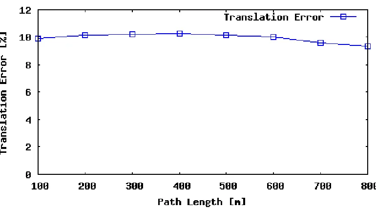
4.3 Sequence 08 translation error as a function of subsequence length. . . 28
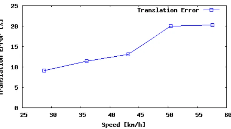
4.4 Sequence 08 translation error as a function of vehicle speed. . . 29
4.5 Sequence 09 rotation error as a function of subsequence length. . . 29
4.6 Sequence 09 rotation error as a function of vehicle speed. . . 30
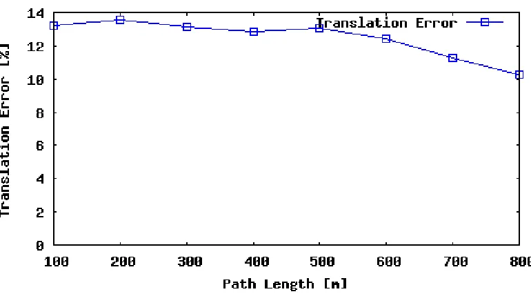
4.7 Sequence 09 translation error as a function of subsequence length. . . 30
4.8 Sequence 09 translation error as a function of vehicle speed. . . 31
4.9 Sequence 10 rotation error as a function of subsequence length. . . 31
4.10 Sequence 10 rotation error as a function of vehicle speed. . . 32
4.11 Sequence 10 translation error as a function of subsequence length. . . 32 4.12 Sequence 10 translation error as a function of vehicle speed. . . 33
4.13 Average sequence rotation error as a function of subsequence length. . 33
4.14 Average sequence rotation error as a function of vehicle speed. . . 34
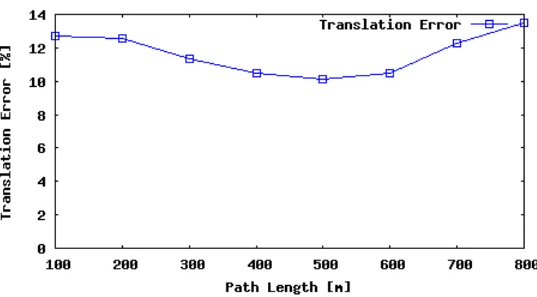
4.15 Average sequence translation error as a function of subsequence length. 34
4.16 Average sequence translation error as a function of vehicle speed. . . 35
4.17 Sequence 08 odometry results compared to ground truth odometry. . 36
4.18 Sequence 09 odometry results compared to ground truth odometry. . 37
4.19 Sequence 10 odometry results compared to ground truth odometry. . 38
4.20 Sequence 00 odometry results compared to ground truth odometry. . 41 4.21 Sequence 01 odometry results compared to ground truth odometry. . 42
4.22 Sequence 02 odometry results compared to ground truth odometry. . 43
4.23 Sequence 03 odometry results compared to ground truth odometry. . 44
4.24 Sequence 04 odometry results compared to ground truth odometry. . 45
4.25 Sequence 05 odometry results compared to ground truth odometry. . 46
4.26 Sequence 06 odometry results compared to ground truth odometry. . 47
4.27 Sequence 07 odometry results compared to ground truth odometry. . 48
4.28 Example flow image from Sequence 01, a highway driving scene. The
neural network incorrectly interprets minimal distance changes, despite the vehicle moving quickly between the two frames that compose the
flow image. . . 48
4.29 Example flow image from Sequence 00, an urban environment. The
flow image shows much greater pixel movement than the highway scene
because objects are closer to the slower moving camera. Because the
urban scenes dominate the dataset, the neural network is unable to
properly learn how to handle highway data. . . 49
3.1 Number of frames per video sequence in the KITTI odometry
bench-mark. Adding mirrored sequences doubles the amount of training data available to the system. . . 20
4.1 Average translation and rotation errors for each video sequence and
method of visual odometry. For each sequence, the average errors are
shown, and the average at the bottom of the table is the weighted
average of the errors based on the number of frames in each sequence. 26
4.2 Timing information for each system. Despite the longer execution time
of the odometry calculation for this work, using FlowNetS and raw
optical flow input greatly reduces the total amount of time required to
produce odometry results. The speedup column expresses how much faster the total execution time of this work is compared to the total
ANN
Artificial Neural Network
CNN
Convolutional Neural Network
GPGPU
General Purpose Graphics Processing Unit
GPU
Graphics Processing Unit
MLP
Multilayer Perceptron Network
RAM
Random Access Memory
ReLU
Rectified Linear Unit
SLAM
Simultaneous Localization and Mapping
VO
Introduction
Visual odometry (VO) is a challenging task that generates information for use in
determining where a vehicle has traveled given an input video stream from
cam-era(s) mounted on the vehicle. In order to estimate motion from a video source, data
must be extracted from individual image frames and related to physical movements,
independent of other moving objects that may be present in the scene. Recently,
a large emphasis has been placed on VO research because of the emergence of
au-tonomous vehicle technology, which relies heavily on inferring physical motion from
digital readings. For the development of the safest vehicle systems, the VO output
must be accurate to feed further into route planning and navigation algorithms.
Traditional algorithms for visual odometry include a method of mapping the
re-sults and placing the vehicle on that map in a process called simultaneous localization
and mapping (SLAM). The distinction between VO and SLAM is that VO provides
raw data for vehicular translation and rotation, and SLAM can use this information
to generate its maps. Despite similar outcomes, SLAM and VO applications use many
different approaches. From particle filtering [3] to feature tracking [4], highly accurate
systems exist, but common themes of slow algorithmic performance and high memory
usage prevent the systems from scaling to requirements needed for extended sessions
of data acquisition and processing. This creates a need for a system capable of rapid
image processing and memory efficiency.
Instead of tracking sparse key points, dense pixel movement can be calculated
using optical flow [5]. Optical flow computes raw pixel movement in both horizontal
and vertical directions and has been widely used for video compression and computer
Figure 1.1: System overview. The red boxes show data, and the blue boxes show opera-tions on the data. At the highest level, consecutive video frames are used to calculate an optical flow image, which is then fed into a convolutional neural network that outputs the odometry information needed to create a map.
between camera updates, an assumption of linear movement between frames is made,
which allows a proportional relation between pixel movements and physical movement
of the camera. Given the advances in the field of deep learning, this thesis proposes
a convolutional neural net (CNN) architecture for producing odometry information
between video frames. Fig. 1.1 depicts the application overview at a high level,
showing the movement of data through the different stages of the system.
The main contributions of this thesis are the following:
• A fully deep learning approach to visual odometry calculation
• A modified FlowNetS [9] architecture, tuned for producing visual odometry data
• An accurate visual odometry system using frame-to-frame visual odometry
This document is organized as follows. Chapter 2 reviews prior literature and its
influence on the proposed design. Chapter 3 describes the setup, data, applications,
and methods of results collection of the proposed design. Chapter 4 describes results
collected from the design and discusses the implications of the results and how they
compare to other systems. Chapter 5 concludes the work and discusses areas for
Background
This chapter provides background information relating to the visual odometry field
and rationale for the work done in this thesis. Section 2.1 explains simultaneous
localization and mapping (SLAM) and various applications and algorithms in visual
odometry. Section 2.2 details deep learning practices and applications related to
computer vision, and more specifically, visual odometry. Section 2.3 describes optical
flow and how it can be leveraged for visual odometry. Section 2.4 lists frame-to-frame
ego-motion estimation systems and their contributions to the visual odometry field.
2.1
Simultaneous Localization and Mapping
Simultaneous localization and mapping (SLAM) is the process of sensing surroundings
to make a map of the environment while also placing an actor, such as a camera on
a vehicle, in that map. Common uses of SLAM include robotic navigation, and more
recently, autonomous vehicles. Although odometry estimation is not new problem,
different SLAM approaches and implementations are constantly emerging as new
technologies become available. Accurate SLAM algorithms must be able to account
for moving objects, speed differences, and steering angle changes to robustly localize
and map the movement path of the actor. All of the works listed in this section use
camera data to perform the localization and mapping tasks.
One approach to SLAM utilized particle filters for grid mapping in the work done
by Grisetti et al [3]. In this approach, the pose of a robot was estimated using a
probabilistic method called particle proposals. Based on the accuracy of sensors on
the robot, particles— or scene estimations— are projected into the environment, and
it is generating. With each movement, particles are eliminated as the robot gains
confidence in its location, and over time, the particles will help the robot create a
full map of where it has traveled. This method improves upon others using particle
filters in that this one often uses an order of magnitude fewer particles for highly
accurate localization and mapping, which in turn decreases the computation time of
the algorithm.
Another approach to SLAM is bundle adjustment, as demonstrated by Konolige
and Agrawal [10]. Inspired by laser-based point tracking techniques, a similar
tech-nique was developed to extract 3D information from stereo image pairs. Key points
were tracked from the image pairs, and pose estimations were calculated from them.
A minimum skeleton of key frames was kept so that localization was indicated as a
pose relative to one of the skeleton frames. Once the pose drifted far from one of
the skeleton frames, it would either localize to the next key frame or compute a new
skeleton frame. This minimalist approach resulted in quick graph solving times and
large loop closure detections, in which the system detects that it has visited the same
location after previously travelling away from it.
A popular methodology for the simultaneous localization and mapping problem
is to track binary image features across frames in a video sequence. Mur-Artal et
al. [4] provided results using ORB-SLAM, which uses ORB feature [11] tracking to
create accurate maps of driving paths from a vehicle-mounted camera. In fact, binary
features extract such important meaning from images that an exhaustive comparison
of image feature detectors and descriptors was performed by Schmidt and Kraft [12]
to determine which binary descriptors provided the most accurate results in the most
efficient amount of time for SLAM algorithms. Their work demonstrated the
perfor-mance of many different image keypoint detectors and descriptors, such as BRISK
(Binary Robust Invariant Scalable Keypoints) [13], BRIEF (Binary Robust
ORB (Oriented FAST and Rotated BRIEF), SIFT (Scale Invariant Feature
Trans-form) [16], and SURF (Speeded Up Robust Features) [17], which all provide different
aspects of information about an image. This analysis resulted in the need for different
types of descriptors or features to advance the field of SLAM research.
2.2
Deep Learning
With the advancement of computational power and graphics processing units (GPUs),
deep learning has seen a massive increase in popularity because of its recent
acces-sibility to researchers without the need for supercomputers. Deep learning has been
able to achieve unprecedented levels of accuracy in tasks such as image classification,
object detection, and other computer vision tasks. By using non-linear functions,
a brain-inspired, data-driven model can be trained to solve tasks after being given
enough examples of inputs with expected outputs. By performing this training, the
model is able to generalize to previously unknown data to make highly accurate
predictions. These neural networks are capable of both discrete classification and
continuous regression solutions, which can be applied in numerous fields, including
odometry estimation for SLAM systems.
The idea of using artificial neural networks to perform intelligent functions has
a long history. In 1969, Minsky and Papert [18] discussed the use of perceptron
networks as a way of creating systems that could compute nonlinear functions by
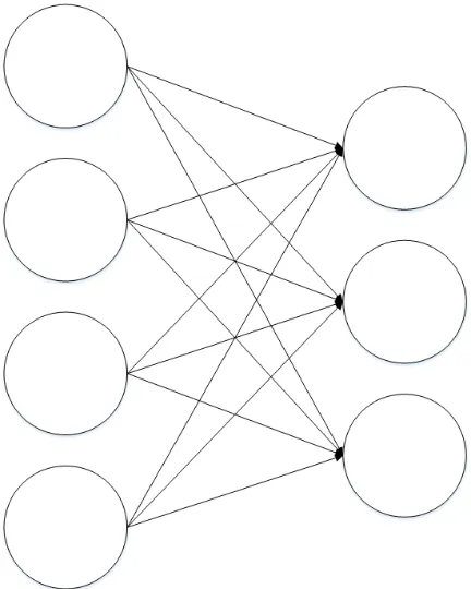
mapping input patterns to output patterns. In a perceptron network, each element
of the output is a weighted sum of each element of the input. An example perceptron
network is shown in Fig. 2.1.
The weights can be adjusted to help generalize the model to correctly classify
or regress data from unknown data samples. After feeding examples to the system,
error could be used to adjust the network weights to minimize error and tune the
Figure 2.1: Example perceptron network.
mapped input directly to output, but this was changed with the advances in processing
power after 1986. McClelland et al. [19] discussed the use of hidden nodes inside of
a perceptron network, effectively creating multilayer perceptron networks (MLPs).
These networks were able to outperform their predecessors, and pave the way for
future contributions to the machine learning field. Years later, after computers were
more capable in terms of memory operations and computational power, the field of
deep learning emerged, which puts more than one hidden layer in neural network
architectures.
The concept of convolutional neural networks was first introduced and successfully
applied by LeCun et al. in 1989 [20]. This type of network was implemented to
recognize handwritten characters in zip codes. By taking shift invariance and spatial
locality into consideration, highly accurate digit classifications were achieved with
minimal network parameters to learn, as compared to MLP networks. Instead of the
Figure 2.2: Convolutional neural network used for character recognition [1].
into image kernels, or filters, that would get updated with error backpropagation.
The convolution operation uses these kernels to produce image response volumes,
which then could be processed with more convolution operations, producing more
meaningful data with fewer parameters. With proper training, the learned filters
in the early convolution stages would resemble the Gabor-like filters of V1 of the
human brain, which tend to mimic simple edge filters. With a smaller number of
parameters, the training process would take significantly less time than it would with
a dense network. At the same time, the model would take up less disk space to store,
although at run time, it is likely to use much more random access memory (RAM)
than the MLP would. Further advances by LeCun et al. [1] focused on gradient-based
learning techniques, and expanded digit recognition to general character recognition.
An example of the character recognition convolutional neural net is shown in Fig.
2.2.
One of the most important contributions to the deep learning field was the use of
general purpose graphics processing units (GPGPU) for massively parallel operations
on massive datasets. First used by Krizhevsky et al. [2], GPGPUs greatly contributed
to the training of the AlexNet architecture on the ImageNet challenge [21]. This
architecture is shown in Fig. 2.3.
By exploiting the parallelism of the convolution operation, and with advances of
Figure 2.3: AlexNet architecture [2].
time of the deep network was significantly reduced to a more manageable amount,
providing high accuracy image classification results in a fraction of the time it would
have with a CPU implementation. Training sessions that previously took weeks to
complete were potentially reduced to a few hours. The use of a GPU has become
necessary in the deep learning field, and it is very rare to find modern deep networks
that were not trained on one.
Gao and Zhang [24] used stacked auto-encoders to produce a system for detecting
loop closures in SLAM algorithms. An auto-encoder is an unsupervised deep
neu-ral network that can be broken into two parts: an encoder network and a decoder
network. The system is trained by connecting the encoder and decoder together to
force the decoder to reconstruct the image or data that was input into the encoder,
as shown in Fig. 2.4.
In some cases, greedy layer-wise training is done, in which one layer is trained
at a time, and once it converges, the next layer is trained with data that comes
from the previously trained layer. After training, the decoder network is removed
so the encoder produces unique feature vectors for different images. In this work,
auto-encoders were used to greedily train three fully-connected layers starting from
an image patch input. The layers contained 200, 50, and 50 hidden nodes for each of
Figure 2.4: Auto-encoder network. The objective of the network is to train the inner weights to reproduce the input data as its output. After training, the last layer is discarded so the network produces feature vectors from the inner layer.
feature vector is extracted from the encoder network, and then concatenated together
to create a unique feature vector for the entire image. Using this type of system, loop
closures were detected by finding the most similar image feature vectors as the camera
moved through space.
Konda and Memisevic [25] used a convolutional neural network to try to solve
the movement part of the visual odometry problem. Unable to get accurate results
from a regression model, they discretized KITTI odometry benchmark data and then
movement was solved as a classification problem instead of a regression problem. The
network processed five consecutive frames of stereo imagery (10 images per sample)
with a convolutional layer for each camera in the stereo configuration. The output
volumes of the two sets up convolutional layers were then combined with an inner
product, and then fed through one more convolutional layer. The output went to a
fully-connected layer and then one more fully-connected layer for a discrete output,
which determined the car angles and speeds between frames. Turns and velocities
were accurately classified, but the resulting driving paths were not as accurate due to
the accumulation of error in an inter-frame odometry estimation system such as this.
Kendall et al. [26] used a convolutional neural network to regress camera poses
GoogLeNet [27] architecture with fine-tuning to convert the classification architecture
into a regression architecture. GoogLeNet is a convolutional neural network with
parallel convolutional operations that compose its novel inception layers. It contains
22 trainable layers and just under 6.8 million parameters to adjust. This network
was originally trained for the ImageNet challenge [21], and it performed better than
the state-of-the-art image classifiers of its time. Kendall et al. utilized this design
and its pretrained weights to adapt it to the application of camera relocalization.
Due to the high accuracy of this system, it was shown that it is possible to regress
real-valued camera pose information, which could potentially translate to camera
movement information in other applications.
2.3
Optical Flow
Optical flow is the task of computing the vertical and horizontal pixel displacement
from one video frame to the next. Traditionally, the optical flow is used for video
compression and activity recognition, but researchers have been able to apply the
motion information to other tasks. Most notably, several different SLAM approaches
use optical flow information to help produce accurate mapping information from frame
to frame.
Before many of the recent optical flow datasets, Brox et al. [28] developed an
algorithm for computing high accuracy optical flow calculations. This method is
robust to noise and demonstrates high accuracy results with smaller angular errors
than optical flow systems before it. On the Yosemite image sequences with and
without clouds, this method outperformed all other comparable optical flow systems.
Even after introducing varying standard deviations of Gaussian noise to the images,
the system still outperformed other works without the noise. This method is one of
the most accurate systems in optical flow calculation.
dataset [6], the KITTI optical flow benchmark [8], the Sintel dataset [7], and the
Flying Chairs dataset [9]. Each of these datasets has a unique challenge for creating
the most accurate optical flow computational system. The Middlebury dataset only
has eight frame pairs with ground truth data to train on, so it cannot be used easily
in deep learning tasks that require many exemplars before converging to a general
solution. The KITTI optical flow dataset has roughly twenty four times as many
samples with ground truth data, but the images are not labeled densely, meaning
that not all pixels are accounted for in the optical flow evaluation. The Sintel dataset
provided over 1,000 training samples with ground truth data, and it also included
frames with and without post-processing effects to evaluate data with and without
theatrical effects, such as motion blurring, between frames. However, this was still
a relatively small number of training samples to use in a deep learning environment.
The Flying Chairs dataset was created specifically for use in training deep neural
networks with almost 23,000 training samples of dense optical flow.
Although not a deep learning approach, Weinzaepfel et al. [29] developed
Deep-Flow, which is a deep neural network-inspired system that calculates optical flow
images between two frames. Using convolutions and pooling, similar to a
convolu-tional neural network, a pyramid of image response maps was created to track patch
displacement in an image. In the highest levels of the pyramid, correspondences were
found between images. Then, based on the locations of the responses, the next level
of the pyramid was accessed to track finer details. This process continued until all
levels of the correspondence pyramid were tracked, which lends itself to the optical
flow image calculation, which is robust to large displacements due to the design of
the process.
Revaud et al. [30] developed DeepMatching, which projected one image into the
coordinate system of another image, by use of dense matching of the image and
generated from a coarse level to progressively finer levels. For the finest correlation
maps, the highest responses tended to accurately predict the movement of small image
patches between the two frames. The movement of the patches could then be
trans-lated into the optical flow image output. This adaptation to the DeepFlow system
shows not only the computation of optical flow, but the transformation properties
between two images, which can relate to movement between frames.
Improving on the previous work on DeepFlow and DeepMatching, Revaud et al.
[31] developed EpicFlow, which produces higher accuracies on optical flow evaluations
from the Sintel dataset. The algorithm uses a novel interpolation method that is
robust to large pixel displacements, boundaries of motion, and occlusions within the
image. It takes edges into consideration, which helps to distinguish fine details of
movement between two different frames. With high optical flow accuracies, the main
drawback is that the run time for the computation exceeds 16 seconds, which is still
much faster than the other optical flow systems it was compared to.
In addition to creating the Flying Chairs dataset, Fischer et al. [9] created
FlowNet, a fully convolutional deep neural network that was trained to produce
opti-cal flow images from a pair of input images. Although it is not the state-of-the-art in
all different optical flow evaluations, its results were comparable to the top methods.
In addition, the run time was one of the fastest for all the evaluations, due to the use
of GPU acceleration for the data. Two different FlowNet architectures were proposed:
one that combined the image pair immediately, and one that filtered the images
sep-arately then combined results later in the network. The FlowNetS architecture used
the former architecture, in which two color images were combined to make a single,
six-channel input. Following this input are ten convolutional layers that ultimately
feed into an upconvolution network that produces a two-channel optical flow image
of the same height and width of the input images. FlowNetC first computes
Figure 2.5: FlowNetS architecture, highlighting convolutional layers before the upconvo-lutional network used for creating the optical flow output.
volumes after three convolutional layers. After, the architecture resembles FlowNetS
in the rest of the convolutions until the output volume is fed into the upconvolution
network. FlowNetS and FlowNetC generalized natural scenes and less realistic scenes,
respectively, showing that each architecture could be used for more accurate results
depending on the type of task or input data at hand. The FlowNetS architecture is
shown in Fig. 2.5.
Relating optical flow to visual odometry, Costante et al. [32] computed dense
optical flow as input to a convolutional neural network that regressed odometry
in-formation. Optical flow was computed using the Brox algorithm [28], then the raw
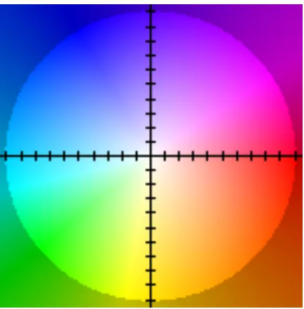
flow image was converted to a color image by using a standard mapping of flow image
to color, which is outlined in the supplementary content of the FlowNet work [9], and
shown in Fig. 2.6. The color image was fed into a convolutional neural network that
regressed six values: three translation components and three rotation components
to address movement and rotations about space in a three-dimensional coordinate
system. This odometry evaluation was more accurate than the previous work that
used deep learning on discretized data [25], and the optical flow data was a large
influence in the performance of the system. This system and the one proposed in
this thesis share many similarities, but the work done in this thesis was developed
Figure 2.6: Color mapping of optical flow vectors. Each of the colors represents how far, and in which direction, a pixel has moved from one image to the next.
2.4
Frame-to-Frame Ego-Motion Estimation
Just as Costante et al. and Konda and Memisevic implemented frame-to-frame
mo-tion estimamo-tion systems, more methods exist that do not use deep learning approaches.
Because the systems only give incremental changes, it is not possible to directly
com-pare these approaches to other SLAM systems that take more factors into account,
such as longer windows of video frames, post-processing of the map, loop closure, and
other such update functions. Frame-to-frame estimation accumulates error over time,
so these approaches are best compared to each other for performance.
Costante et al. evaluated their different convolutional neural network architectures
against two different frame-to-frame methodologies. The first was the StereoScan
al-gorithm [33] by Geiger et al., which used 3D reconstruction from stereo images to
produce visual odometry information. The second was a support vector machine
(SVM)-based model for predicting visual ego-motion by Ciarfuglia et al [34]. The
SVM was trained on histograms of optical flow, generated from consecutive frames
incremen-tal changes in motion based on only the optical flow between two images, which
makes them more comparable to each other than other SLAM algorithms. This work
presents a similar system, so for analysis, it will be compared to these frame-to-frame
estimation systems.
In the work done by Geiger et al. [33], the StereoScan algorithm was developed to
generate 3D maps in real-time based on stereo video sequences. By algorithmically
calculating the 3D disparity between video frames, a three-dimensional reconstruction
of the environment could be created. This system was adapted into a visual
odom-etry system in the work by Costante et al. [32] by relating the disparity between
video frames to physical motion instead of tracking the static environment. This is
called VISO2-M in the comparison to the convolutional neural network proposed by
Costante et al.
In the SVM-based visual odometry system [34], movement between frames was
”learned” in a supervised method using optical flow imagery and ground truth
la-beling. This method, named SVR-VO, was one of the first methods that did not
use a geometric calculation approach to estimating movement between video frames.
It was shown that learning-based approaches, such as SVM or Gaussian processes
were capable of performing as well or better than the geometric systems while also
Visual Odometry Estimation
This chapter describes a system for estimating visual odometry using frame-by-frame
ego-motion estimation from optical flow images. Section 3.1 details the convolutional
neural network architecture for the system. Section 3.2 describes the input data for
the network and augmentation used for increasing the number of samples for training
the network as well as the output that is extracted from the network. Section 3.3
describes the overall application of the system for visual odometry estimation. Section
3.4 details how results are collected from the system and how accuracy is measured
for the model.
3.1
Convolutional Neural Network Architecture
Several existing CNN architectures were explored in efforts to leverage
state-of-the-art image classification networks for visual odometry estimation. CaffeNet [35],
AlexNet [2], and GoogLeNet [27] were considered, but experimental results
deter-mined that these were not the best choice in this type of application. For AlexNet
and GoogLeNet, the last layers of the networks were removed and replaced with the
dense layers needed to regress the odometry information, and then the pre-trained
networks were fine-tuned to this application. CaffeNet was both fine-tuned with
pre-trained weights and pre-trained from randomly initialized weights. All of these networks
were unable to converge to comparable results to other leading works in this field.
In this system, a convolutional neural network architecture based on FlowNetS
[9] is introduced for the task of visual odometry estimation. The architecture
orig-inally estimated optical flow, so it was taken one step further to compute physical
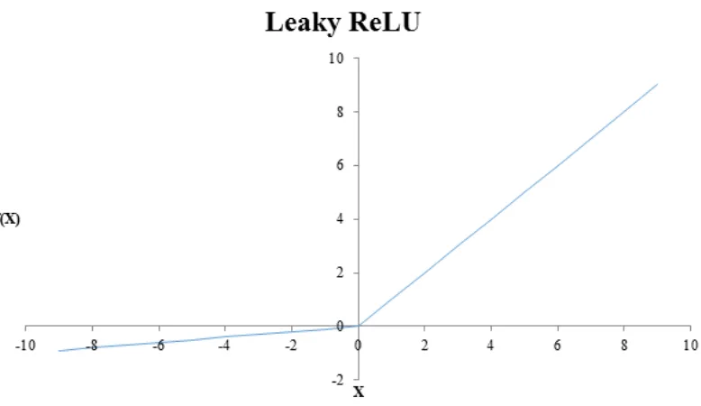
Figure 3.1: Leaky ReLU nonlinearity with negative slope of 0.1.
a flow image taken from the original FlowNetS network, and fed into this network to
produce the odometry results. FlowNetS was chosen for producing optical flow input
data because of its better performance in natural scenes relative to FlowNetC and
because of its fast computation time compared to many other optical flow systems.
The network is comprised of ten convolutional layers and two fully connected layers.
The network gradually reduces the image size with strided convolutions until a fully
connected layer with 1024 nodes is reached. After this layer, dropout [23] with a
prob-ability of 50% is used before the two output nodes, which are the regression values
for the displacement and rotation angle for each flow image. After all convolutions
and the first fully connected layer, the leaky rectified linear unit (leaky ReLU) [36]
nonlinearity with a negative slope of 0.1 was applied, just as it was in the original
FlowNetS architecture. This nonlinearity is shown in Fig. 3.1.
The entire network was developed using the Caffe deep learning framework [35],
using the same version as supplied by the FlowNet work. A visualization of the
Figure 3.2: Convolutional neural network architecture based on the contractive part of FlowNetS.
3.2
Training Data
For this system, ego-motion is estimated from two consecutive video frames. Instead
of inputting the two images directly into the network, a flow image is computed using
the FlowNetS architecture, and then that result is used as the network input. Each
of these flow images represents the change between two video frames, so the
corre-sponding motion differentials can be computed from the ground truth provided by
the KITTI odometry dataset [8]. The KITTI dataset gives 11 video sequences with
ground truth data for each frame in the videos for training, and 11 more sequences
without ground truth data to be used in the online evaluation of a visual odometry
system. In this work, and in other works of similar function, the 11 sequences without
ground truth are ignored, and instead, sequences 08, 09, and 10 are used for
evalu-ation, and sequences 00 through 07 are used for training and fine-tuning the visual
odometry system. The number of frames in each of the training and testing sequences
are given in Table 3.1. Three examples of images in dataset are shown in Figs. 3.3,
3.4, and 3.5. Examples of flow images, colored for visual representation, are shown
in Figs. 3.6, 3.7, and 3.8. The flow images show how pixels should move for straight
vehicle movement, left turns, and right turns, respectively. Although these are color
images, they are only shown for human visualization. Raw, two-channel optical flow
images are used as input to the system.
transfor-Table 3.1: Number of frames per video sequence in the KITTI odometry benchmark. Adding mirrored sequences doubles the amount of training data available to the system.
Phase Sequence Frames
Training 00 4541
01 1101
02 4661
03 801
04 271
05 2761
06 1101
07 1101
Testing 08 4071
09 1591
10 1201
Figure 3.3: Example frame from KITTI Sequence 08.
[image:32.612.106.542.113.483.2]Figure 3.5: Example frame from KITTI Sequence 10.
Figure 3.6: Example optical flow image depicting straight movement forward.
Figure 3.8: Example optical flow image depicting a right turn. Based on the vector mapping, the blue color means that pixels moved left, which is to be expected when the camera physically moves right.
mation matrices that transform the first frame of a video sequence into the coordinate
system of the current frame. The transformation matrix is composed of a rotation
matrix with a translation vector concatenated to it. The rotation matrix is defined
in (3.1). The translation vector is defined in (3.2). From this set of data,
incremen-tal angle changes are calculated by decomposing the rotation matrices to find the
differences between the angles, as shown in (3.3).
Ri =
Ri,1 Ri,2 Ri,3
Ri,4 Ri,5 Ri,6
Ri,7 Ri,8 Ri,9
(3.1)
Ti =
Ti,X Ti,Y Ti,Z (3.2)
∆Θi = arctan (Ri,3, Ri,1)−arctan (Ri−1,3, Ri−1,1) (3.3)
be-tween the translation portions of the transformation matrices, as shown in (3.4).
∆di =
p
Σ(Ti−Ti−1)2 (3.4)
For every flow image input, an angle and a distance are regressed to represent
the displacement and orientation change of the camera. This converts the global
transformation data into an ego-motion format in which small changes are
accumu-lated over time. To increase the number of training samples, every image was also
flipped horizontally and the ground truth angle was negated to reflect the change.
This causes the dataset to have equal numbers of left and right hand turns with equal
magnitudes, hypothetically preventing the network from learning to prefer one type
of turn over the other.
3.3
Mapping Frame-to-Frame Odometry
The displacements and angles computed for the flow images are independent of the
previous or next frames in the video sequence. This means that each flow image will
produce the same results every time it is input, regardless of the order the images
are input to the CNN. For arbitrary sequences of flow images, a position in global
space can be accumulated using the incremental distance and angle changes, relative
to the current camera position. At the start of every sequence, the camera position
is initialized at the origin of an XZ coordinate system, with X and Z as the 2D
movement plane. The Y-axis for elevation was left out because the differences in
elevation were at least an order of magnitude smaller than the movement in the other
axes. Starting from the origin, the next position is accumulated by applying the angle
and displacement to the current position, using Algorithm 1. Intermediate results are
saved to help plot the driving path and to convert the data into a format that can be
3.4
Evaluation
For each flow image in a video sequence, the angle and displacement are extracted
from the network. As described in 3.3, these values are used to incrementally build
a map, but to compare results to the KITTI benchmark, the output must be in the
format of a 3x4 transformation matrix that transforms the first frame of the video
sequence into the coordinate system of the current frame. Let R be a 3x3 rotation
matrix, and T be a 3x1 translation vector, such that the concatenation of R and T
create the 3x4 transformation matrix as described in the KITTI benchmark. As the
relative location is calculated for each flow image, the angles are saved relative to the
overall global map. Now, because the global angles and translations are calculated,
they can be converted into the transformation matrix format. Assuming no changes in
elevation, Algorithm 2 is used to calculate these matrices for each video frame. The
subtraction of 90 degrees is included because Algorithm 1 introduced the angle to
calculate the correct X and Z positions, but the coordinate system of the benchmark
is assumed to generate the results.
Once the rotation matrices are computed, they are evaluated using the KITTI
evaluation software. This software computes the translation and rotation errors for
the visual odometry system as functions of both subsequence length and vehicle speed.
This evaluation provides standard results used to quantifiably compare different
vi-sual odometry systems using the same dataset. The evaluation plots the vehicle
paths and the translation and rotation errors, as well as an overall average error for
the translations and rotations. It is meant to provide transparency for the evaluation
of the driving sequences that have no ground truth data provided, but in this case,
only sequences 08 through 10 are evaluated to compare with other systems that use
frame-to-frame odometry estimation with provided ground truth data. The average
translation and rotation errors are used to compare the performance of different
Results
After training the convolutional neural network to produce rotation and translation
information from optical flow images, the network was evaluated on three driving
sequences that were left out of the training data. These sequences include suburban
environments with minimal dynamic objects, such as pedestrians or other driving
cars. The KITTI evaluation software was slightly modified to provide results only for
the three testing sequences. For each sequence, six metrics are recorded: total average
translation error, total average rotation error, average translation error as a function
of subsequence length, average translation error as a function of vehicle speed, average
rotation error as a function of subsequence length, and average rotation error as a
function of vehicle speed.
Table 4.1 shows the total average translation and rotation errors for each sequence.
Results of other works, as represented in the FlowNet work, are shown in comparison
with this system. VISO2-M uses a geometric approach, SVR VO uses a support
vector machine approach, and P-CNN uses a convolutional neural network approach
for visual odometry estimation.
Table 4.1: Average translation and rotation errors for each video sequence and method of visual odometry. For each sequence, the average errors are shown, and the average at the bottom of the table is the weighted average of the errors based on the number of frames in each sequence.
VISO2-M SVR VO P-CNN VO This Work
Seq Trans Rot Trans Rot Trans Rot Trans Rot
[%] [deg/m] [%] [deg/m] [%] [deg/m] [%] [deg/m] 08 19.39 0.0393 14.44 0.0300 7.60 0.0187 9.98 0.0544
09 9.26 0.0279 8.70 0.0266 6.75 0.0252 12.64 0.0804
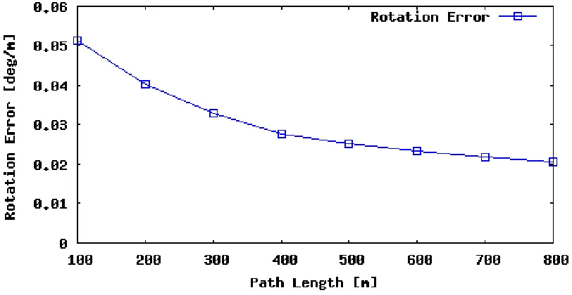
Figure 4.1: Sequence 08 rotation error as a function of subsequence length.
In addition to the average error per sequence and total average, the more detailed
translation and rotation errors are compiled into graphs via the KITTI evaluation
software. Figures 4.1, 4.2, 4.3, and 4.4, depict errors for Sequence 08, Figures 4.5,
4.6, 4.7, and 4.8 for Sequence 09, 4.9, 4.10, 4.11, and 4.12 for Sequence 10, and 4.13,
4.14, 4.15, and 4.16 for the average of all three sequences.
It should be noted that each of the sequences are different lengths, with Sequence
08 having 4071 frames, Sequence 09 with 1591 frames, and Sequence 10 with 1201
frames. Because of the difference in video lengths, the average error will be most
biased toward Sequence 08 for all measurements. For the rotation error over
sub-sequence length, the error appeared to decrease as larger numbers of frames were
considered. This is likely because the error is averaged out over the larger
subse-quence lengths. Relative to the number of frames where the vehicle travels straight,
there are few frames where the vehicle makes a turn. For all errors with respect to
vehicle speed, error tends to increase with faster speeds because there are significantly
fewer samples of driving data with speeds that high, giving more magnitude to the
Figure 4.2: Sequence 08 rotation error as a function of vehicle speed.
[image:40.612.137.522.442.656.2]Figure 4.4: Sequence 08 translation error as a function of vehicle speed.
[image:41.612.129.531.446.657.2]Figure 4.6: Sequence 09 rotation error as a function of vehicle speed.
[image:42.612.137.522.443.656.2]Figure 4.8: Sequence 09 translation error as a function of vehicle speed.
[image:43.612.135.530.446.656.2]Figure 4.10: Sequence 10 rotation error as a function of vehicle speed.
[image:44.612.136.523.442.656.2]Figure 4.12: Sequence 10 translation error as a function of vehicle speed.
[image:45.612.129.531.446.657.2]Figure 4.14: Average sequence rotation error as a function of vehicle speed.
[image:46.612.136.524.444.656.2]Figure 4.16: Average sequence translation error as a function of vehicle speed.
only varying a few percentage points, and thus showing that the system was
consis-tent in predicting displacement between video frames. The accuracy of this system
does not exceed the accuracy of other frame-to-frame ego-motion estimation systems,
but it is still comparable to the state-of-the-art system, P-CNN VO, especially for
Sequence 10, in which this work has 10.77% accuracy over P-CNNs 21.23% accuracy
in translation. Accounting for these errors, the entire paths generated by this system
are shown in Figs. 4.17, 4.18, and 4.19.
Due to the nature of inter-frame odometry systems, error accumulates over the
length of the sequence. Although most predictions may be correct, rotation error will
distort parts of the overall path and cause the translation error to rise significantly
because no methods are in place to correct error once it is introduced to the system.
Despite the integration error from this system, the displacement scale of each
pre-dicted path seems to be accurate, as shown by the strong resemblance of the shape of
the predicted path compared to the ground truth path when ignoring larger rotation
errors.
turns in the negative X-direction of the graph. This sequence is mainly a suburban
track, but at the turns where the rotation error is not as accurate, there is an absence
of buildings, and instead there were trees in the distance, farther away than where
buildings would have been relative to the car. In terms of the optical flow, the pixel
movements would be much smaller than if the buildings were there, which is likely to
explain why the magnitude of the turning angles around those corners were less than
90◦. As shown by the shape of the rest of the map, there were minimal translation
and rotation errors, showing that the system worked best in a consistently suburban
setting.
In Sequence 09, the environment contained hills and more spaced out buildings
than were in Sequence 08. As shown in the predicted path of Sequence 09, the
first large turn was not as wide as what the ground truth shows, and this is likely
explained by the environment in those video frames. Just as in Sequence 08, the
distant background of trees in those frames would cause the optical flow magnitudes
to appear smaller than the actual turning magnitude of the car.
In Sequence 10, the car drives through narrow roads with high walls, so the sides
of the video frames closest to the camera show more movement than would normally
be observed in suburban driving. Because of the proximity of the larger optical
flow magnitudes to the middle of the frame, the system responds by interpreting the
movement as a tighter left turn than the ground truth shows it should be.
Overall, the KITTI odometry dataset is comprised mostly of suburban driving
examples and very few examples with distant backgrounds. It seems that accurate
results, specifically for rotations, are dependent on the availability of suburban scenes
in the video sequence. The displacements seem to be accurate throughout, but that
could mostly be attributed to the camera frame rate, and the fact that the
vehi-cle cannot move farther than a few meters in 100 ms, even at high velocities. The
informa-tion, so the neural network was able to generalize the distances well. The amount of
turning data compared to the amount of data where the vehicle is driving straight is
considerably underrepresented, causing difficulty for the neural network to generalize
well to the turning information.
With a deep neural network system, such as this, it is important to ensure that the
network is not overfitting, or ”memorizing,” the training data. If this was the case, it
would be expected that the training sequence predictions would almost exactly match
the ground truth, producing near-perfect maps. Figs. 4.20 through 4.27 show the
mapping results of Sequences 00 through 07.
In Fig. 4.20, scale and rotation drift are evident in the mapping. Several of the
path shapes are clearly drawn by the system, but turns, especially on the western
side of the chart, were challenging for the network to reproduce. In Fig. 4.21, there is
a massive difference in scale and slight difference in rotation. This sequence contains
only highway driving data with few landmarks and structures near the vehicle while
it moves. Because of the disproportionate number of suburban driving scenes to
highway driving scenes, the odometry system learned how to scale its results only to
scenarios where there are large landmarks close to vehicle while it moves. This means
that large optical flow will create larger displacements, but the highway driving had
artificially smaller optical flow results because of its wide area of view and minimal
change in scenery despite the actual distance traveled. This can be seen in Fig.
4.28, which is the optical flow representation of one of the frames in Sequence 01.
Most of the image is white, which is interpreted as pixels did not move, signifying
minimal distance change between frames, contrary to the great distance actually being
maneuvered. This contrasts the flow images from urban environments, in which pixels
are rapidly moving when the vehicle is traveling slow speeds because of the proximity
of buildings and objects to the cameras. Fig. 4.29 shows a typical urban environment
Figure 4.27: Sequence 07 odometry results compared to ground truth odometry.
Figure 4.28: Example flow image from Sequence 01, a highway driving scene. The neural
Figure 4.29: Example flow image from Sequence 00, an urban environment. The flow image shows much greater pixel movement than the highway scene because objects are closer to the slower moving camera. Because the urban scenes dominate the dataset, the neural network is unable to properly learn how to handle highway data.
In Fig. 4.22 the system had great difficulty in predicting angles, but the scale of
displacements seemed appropriate compared to the ground truth path. Fig. 4.23 had
a small amount of scale and rotational drift, but the resulting map was very similar
to the actual driving path. Fig. 4.24 shows the results of the vehicle driving in a
straight line. The visual odometry system drifted to the left with some scaling issues,
most likely due to the placement of buildings relative to the cameras on the car. This
was a very short sequence so the neural network did not have a lot of exposure to
this specific scene.
Figs. 4.25, 4.26, and 4.27 all show that the system had the capability of predicting
the correct scale of movement for suburban driving environments, but turns were still
problematic. Most of the training data places buildings at specific distances away
from the vehicle, so the neural network associates the presence of the buildings with
moving in a straight line. Especially in Fig. 4.26, there is a lot of left-hand turn
drift because the layout of this short scene did not match the much longer training
examples with specific environment layouts.
As shown in all of the training data examples, the neural network learned to
gen-eralize the odometry task for the dominant training examples in the dataset. For
con-sisted of suburban driving scenes that the system was more likely to predict correctly.
The training path maps show that the system was not overfitting to any particular
training set because the same turning and scaling mistakes were made in both
train-ing and testtrain-ing examples. There are two main sources of error that stem from the
dataset itself. There is a disproportionate amount of suburban driving data to any
other scene type, and there are not enough turns in the dataset for the convolutional
neural network to properly estimate the magnitude of an angle between video frames.
This causes the system to have a bias toward learning how to navigate only suburban
scenes in straight lines, which is very evident in the map of Fig. 4.17.
Although the KITTI benchmark evaluates performance based on the total map,
it does not consider the performance of the incremental predictions made by inter
frame odometry systems. For this system, the distributions of incremental errors
were analyzed. Fig. 4.30 shows the distributions of translation error for each of the
three test sequences. Fig. 4.31 shows the rotational error distributions for the three
test sequences.
As shown in Fig. 4.30, the error between predicted and ground truth translations
stayed consistently within 2 m, except for a single data point that exceeded an error of
4 m. These results are consistent with what was shown in the generated environment
maps. The map scale was generally correct, but the rotations caused distortions in
the map output. Analysis of the rotation error distribution in Fig. 4.31 shows this
trend. For the most accurate system, errors within 5 degrees would be preferable, but
this system generated errors ranging from close to 0 degrees up to 140 degrees of error.
This error manifests in the maps by distorting and twisting the maps away from the
ground truth values. Although there are still a majority of correct predictions, it is
the accumulation of all error that causes the end result of a distorted map. Due to
the translation errors being fairly consistent, the main source of error comes from the
Table 4.2: Timing information for each system. Despite the longer execution time of the odometry calculation for this work, using FlowNetS and raw optical flow input greatly reduces the total amount of time required to produce odometry results. The speedup column expresses how much faster the total execution time of this work is compared to the total execution time of each system, using (4.1).
Optical Flow RGB Odometry Total This Work
Calculation Conversion Calculation Execution Speedup [s/frame] [s/frame] [s/frame] [s/frame]
VISO2-M 14.812 0.210 0.063 15.085 23.831
SVR-VO 14.812 0.210 0.112 15.134 23.908
P-CNN 14.812 0.210 0.041 15.063 23.796
This Work 0.271 0.000 0.362 0.633 —
In addition to accuracy measurements, timing measurements were collected as
well. Because this system uses convolutional neural networks from end to end, it
utilizes the speed advantages that neural networks and GPU acceleration have to
offer. Timing results from previous works did not factor in the steps to generate
optical flow information used for the odometry calculation steps. Using raw optical
flow from FlowNetS dramatically reduces the run time of the application, and prevents
a timing penalty that comes from converting optical flow to color images, as was done
in the comparison models. Table 4.2 shows the timing results of this work compared
to the other works. Speedup is used to measure how much faster this work runs than
the other, and it is shown in (4.1).
speedup= told
tnew
(4.1)
For odometry timing results, the best results were picked out of the work by
Costante et al. To measure optical flow timing for comparison works, the Brox
algo-rithm was timed for 1000 random consecutive image pairs, and the fastest observed
timing was used for comparison. For this work, the average timing for the same
1000 image pairs was used. The other works used a step to convert optical flow
images was used. For this work, the average timing of odometry collection of 1000
optical flow images was collected, and then for all works, the total execution time
is the sum of the previous timing results. Using best-case results from the other
works, and average timing results from this work, it is shown that this work will run
with a 23.796x speedup over the next fastest application, thus making this the fastest
Conclusion
The aim of this thesis was to introduce a novel system for frame-to-frame ego-motion
estimation in a driving dataset. An end-to-end system for using raw optical flow input
to produce incremental odometry information was successfully implemented. A
mod-ified version of the FlowNetS architecture was trained on eight of the sequences in the
KITTI odometry evaluation dataset, and then test results were collected from three
sequences previously unseen by the system. The accuracy of the odometry system did
not exceed the state-of-the-art in all aspects, but the results were still comparable.
This system differs from others of similar function for two main reasons. It uses raw
optical flow images instead of color image representations of the optical flow, and its
weights did not have to be initialized with semi-supervised pre-training. This removes
two steps from the network training process, which takes a significant amount of time
with large enough architectures and quantities of images. Overall, using convolutional
neural networks for the entire system drastically reduces the amount of time needed
to go from camera input to odometry output.
Although the results are comparable, there are several limitations that can be
addressed in future work to improve the system altogether. First, more iterations
of trial and error for number of parameters could be explored. Numerous trials
were performed until the current network architecture was selected, but this was
not an exhaustive search for the best hyperparameters. The use of Caffe made a
hyperparameter sweep difficult to perform due to its use of static text files for network
structure. This was managed in this thesis by using BASH scripting to copy and edit
files on the fly, but a more versatile language for dynamic network configuration and
Next, regressing more values would most likely help improve accuracy in
trans-lations and rotations. As shown in the work by Costante et al. [32], high accuracy
estimations were achieved by regressing three values for camera center displacement
and three values for camera rotation along the three axes. This work estimates only
the magnitude and direction of movement in two values fixed in a two-dimensional
plane. Although the axis of elevation did not show a significant different in accuracy
between this and other works, it is possible that accounting for it would bring the
system accuracy closer to that of the state-of-the-art.
Other experimental setups were considered, but they were not tested. It is possible
that using a median filter on multiple optical flow images could create predictions
that minimize large rotational errors. Despite the potential accuracy gains, this
would introduce larger errors when the vehicle is turning because for quick turns,
the median filter would bias predictions toward driving straight. Alternatively, using
multiple optical flow images as input to the convolutional neural network could help
to reduce rotational error. This was not a testable experiment because any more
data used as input would have exceeded the amount of memory available on the
graphics cards used for training. This would also be true for using stereo imagery
instead of monocular imagery for input. For future research, these scenarios could be
[1] Y. Lecun, L. Bottou, Y. Bengio, and P. Haffner, “Gradient-Based Learning Applied to Document Recognition,”Proceedings of the IEEE, vol. 86, no. 11, pp. 2278–2324, 1998. [Online]. Available: http://ieeexplore.ieee.org/lpdocs/epic03/ wrapper.htm?arnumber=726791
[2] A. Krizhevsky, I. Sutskever, and G. E. Hinton, “ImageNet Classification with Deep Convolutional Neural Networks,” Advances In Neural Information
Pro-cessing Systems, pp. 1–9, 2012.
[3] G. Grisetti, C. Stachniss, and W. Burgard, “Improved techniques for grid map-ping with Rao-Blackwellized particle filters,” IEEE Transactions on Robotics, vol. 23, no. 1, pp. 34–46, 2007.
[4] R. Mur-Artal, J. M. M. Montiel, and J. D. Tardos, “ORB-SLAM: A Versatile and Accurate Monocular SLAM System,” IEEE Transactions on Robotics, vol. 31, no. 5, pp. 1147–1163, 2015.
[5] B. Horn and B. Schunck, “Determining optical flow: A retrospective,”Artificial Intelligence, vol. 59, no. 1-2, pp. 81–87, 1993.
[6] S. Baker, D. Scharstein, J. P. Lewis, S. Roth, M. J. Black, and R. Szeliski, “A database and evaluation methodology for optical flow,”International Journal of
Computer Vision, vol. 92, no. 1, pp. 1–31, 2011.
[7] D. J. Butler, J. Wulff, G. B. Stanley, and M. J. Black, “A naturalistic open source movie for optical flow evaluation,” inLecture Notes in Computer Science (including subseries Lecture Notes in Artificial Intelligence and Lecture Notes in
Bioinformatics), vol. 7577 LNCS, no. PART 6, 2012, pp. 611–625.
[8] A. Geiger, P. Lenz, and R. Urtasun, “Are we ready for autonomous driving? the KITTI vision benchmark suite,” in Proceedings of the IEEE Computer Society
Conference on Computer Vision and Pattern Recognition, 2012, pp. 3354–3361.
[9] P. Fischer, A. Dosovitskiy, E. Ilg, ..., and T. Brox, “FlowNet: Learning Optical Flow with Convolutional Networks,” Iccv, p. 8, 2015. [Online]. Available: http://arxiv.org/abs/1504.0685
[10] K. Konolige and M. Agrawal, “FrameSLAM: From bundle adjustment to real-time visual mapping,” IEEE Transactions on Robotics, vol. 24, no. 5, pp. 1066– 1077, 2008.
[11] E. Rublee, V. Rabaud, K. Konolige, and G. Bradski, “ORB: An efficient alternative to SIFT or SURF,” in Proceedings of the IEEE International