Automatic Variance Control and Variance Estimation Loops
T.J.Moir
I.I.M.S., Massey University Albany Campus, Auckland, N.Z.
[email protected]
Abstract
A closed loop servo approach is applied to the problem of controlling and estimating variance in non-stationary signals. The new circuit closely resembles but is not the same as, automatic gain control (AGC) which is common in radio and other circuits. The closed loop nature of the solution to this problem makes this approach highly accurate and can be used recursively in real time.
1 Introduction
In applications which use adaptive filters, usually some estimate of variance is required if a Least-Mean Squares (LMS) algorithm is used for weight vector estimation [1]. Normally a window or moving window of data can be used and the sample variance computed. A finer approach is to update the variance recursively. That is, (assuming large k) for a sample variance
σ
k2 of k samples of zero-mean datay
kσ
k 2=
1
k
y
i 2i=1 k
å
(1)the recursive equivalent is given by [2]
]
[
1
2 1 2 2 1 2 − −+
−
=
k k kk
y
k
σ
σ
σ
(2)For stationary signals the recursive variance estimator converges asymtotically as
k
→
∞
. A similar method can be used for estimating the mean recursively [2]. However, if the signal is non-stationary then (2) must be able to track the time-varying variance. The problem is that with large k, equation (2) pays little attention to new information and ‘switches off’. Sometimes a factor of safety is used and the variance magnitude is under-estimated to allow for any sudden changes, or if the dynamic range of the signal (as is the case with speech) is known a worse case upper estimate can be used. In the case of the LMS algorithm if the variance is under-estimated the algorithm can become unstable due to the step size becoming too large. Conversely if the variance is over-estimated the convergence of the LMS algorithm may well be too slow [1]. This basic problem has been recognised in [3] where the authors alter the LMS algorithm to implicitly include automatic gain control. It is usual in the literature to use some form of exponential weighting of past data to track the variance. This facilitates the use of a ‘forgetting factor’. For example it is often proposed to use2 2
1
2
(
1
)
k k
k
βσ
β
y
where 0<
β
<1 is the forgetting factor which controls the bandwidth and the time constant of the first order recursive digital filter. For a typical speech signal, usingβ
=0.95 can be made to work although the estimate is not very smooth. Increasingβ
gives smoother estimates at the expense of worse tracking.The implicit approach in [3] uses a forgetting factor approach similar to the above. Whilst methods like these can be made to work for certain applications, they are generally of an ad-hoc nature and are a compromise between smoothness of the estimate and tracking ability. The approach used here can be used for accurate tracking of variance or better still to accurately define the variance of a signal with a pre-defined set-point. The philosophy is similar to that used in radio receivers where an AGC boosts the radio frequency signal to a useful power for later amplification and detection. Hence this approach is proposed as a front end to adaptive algorithms rather than an implicit change to the LMS algorithm itself, such as has been proposed in [3]. An automatic gain control strategy has been proposed in [4] which improves the performance of an LMS adaptive filter but it too uses forgetting factors and is highly non-linear.
2 Automatic Variance Control
The automatic variance control (AVC) described here is essentially a form of AGC calibrated to variance rather than amplitude or average power rather than voltage. Whilst it would seem obvious that an AGC may well suffice it should be recalled that AGCs are largely non-linear and would not result in accurate tracking. Although the AVC uses non-linear elements, its tracking ability is entirely linear with theoretically zero steady-state error to a step change in variance.
The block diagram of the AVC is shown in Figure 1. It comprises a pure squarer, a linear multiplier, a summing junction (with set-point) and an integrator.
Figure 1 Automatic Variance Control block diagram
The operation of the circuit is essentially as follows.
squarer will also change momentarily and this is in turn fed into the squarer. When a signal is squared it produces a dc term plus higher harmonics. The higher harmonics are filtered by the integrator and any change in dc from the squarer output produces either a larger or smaller error from the summing junction which is in turn integrated. The integrator will either ramp up or down to scale the input signal to a pre-defined amount defined by v(t). A squarer is used within the loop as opposed to a modulus detector normally used in AGC loops since this provides the suitable scaling for variance rather than amplitude.
3 Steady-State Analysis
The analysis follows from the block diagram of Figure 1. The input
f
i(
t
)
can be either deterministic or stochastic bust must be non-zero in the long term and free from dc. The integrator output becomesy
(
t
)
=
K e
ò
(
t
)
dt
(4)The error signal is defined as
)
(
)
(
)
(
t
v
t
u
t
e
=
−
(5)where u(t) is the squarer output which when combined with the multiplier output results in
))
(
)
(
(
)
(
2t
y
t
f
t
u
= i (6)For any close loop system the gain K must be as high as possible for a given bandwidth. From basic servo theory, assuming K>>1 gives an error
e
(
t
)
→
0
and from (5) and (6))
(
))
(
)
(
(
2t
v
t
y
t
f
i → (7)However, since
(
)
(
t
)
y
(
t
)
i
f
t
o
f
=
we must have)
(
)
(
2
t
v
t
f
o→
(8)This can be interpreted as follows for two classes of input signal.
3.1 Deterministic input signals
For a set-point variance v(t)=1 and input waveform
f
i(
t
)
consisting of a sine wave of unity amplitude, thefrom basic trigonometry, produces a dc term and a component at
2
f
u Hz. Just as with a phase-locked loop, the2
f
u term must be sufficiently attenuated by the bandwidth of the loop to avoid distortion. This is achieved by ensuring that the unity gain crossover frequency of the integrator is at least ten times smaller than the2
f
u component. Hence the bandwidth of the AVC must be chosen to be at least one tenth of the lowest frequency of interest. A phase-locked loop can operate at much higher bandwidths since the input frequency is usually in the kHz or MHz region. Clearly for our applications, since the input frequencies are usually baseband, the AVC, like an AGC, is a slow acting control loop with a practical bandwidth at most of a few tens of Hz .3.2 Random input signals
Taking expectations of both sides of (8) gives
)]
(
[
)]
(
[
f
2t
E
v
t
E
o→
(9)The variance set-point v(t) is deterministic and clearly
E
[
v
(
t
)]
=
v
(
t
)
.Hence from (9) it is seen that the random output signal will be scaled so that its variance tracks the set-point. For example, a zero-mean white noise input of unit variance and a set-point variance of unity will result in an output variance of unity and the statistical characteristics will remain otherwise unchanged. For the same set-point, if the input variance slowly increases or decreases, the output variance will stay at unity.
For a time-varying input of say a speech waveform, the AVC will not have sufficient bandwidth to respond to periods of non-speech. This is a positive result since any amplification of background noise is undesirable as is any distortion of the speech ‘envelope’.
4 Estimation of input variance
With slight modification, the AVC can be used as an accurate recursive method of estimating variance and will not suffer from the same disadvantages as discussed for equations (1) and (2). This method like all closed loop methods is only limited by the bandwidth of the loop. A fundamental assumption is made here that the integrator output is statistically independent of the input signal and we can write
)]
(
[
)]
(
[
)]
(
[
f
2t
E
f
2t
E
y
2t
E
o=
i . (10)This assumption is born out by the fact that the bandwidth of the AVC is small and the integrator smooths out any high frequency components. For stationary input signals the integrator output will be a constant in steady-state and effectively
y
(
t
)
→
y
o. A similar argument is used in analysis of the weights for an LMS algorithm[1].The input variance can now be computed by re-arranging (10) and substituting set-point variance instead of
)]
(
[
f
2t
E
o via (9). Then)]
(
[
)
(
)]
(
[
2 2t
y
E
t
v
t
f
Which requires the division of the set-point with the mean squared integrator output. To avoid division, which is computationally time consuming a further closed-loop system is used as shown in Figure 2 which consists of an integrator, a set-point and a multiplier.
Figure 2. Variance Estimation loop
An additional squarer is required outside the AVC loop from the integrator which obtains
y
2(
t
)
. The analysis of the loop of Figure 2 follows closely the method used previously. From the block diagram the error signal is given by)
(
)
(
)
(
)
(
2 22
t
v
t
y
t
y
t
e
=
−
(12)Where
y
2(
t
)
is the integrator output in Figure 2.Assume the integrator gain K>>1 and the error signal
e
2(
t
)
→
0
. This results in)
(
)
(
)
(
22
t
y
t
v
t
y
→
(13)5 Simulation Results
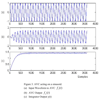
[image:6.612.74.449.264.640.2]The AVC and variance estimation loops can be implemented either in digital or analogue form. For this work the loops were implemented in software and several different signal types were tested. For convenience, a set-point of unity was used for all cases. For a sine wave input of unity amplitude and unity set-set-point the AVC gave an output of a sine wave with magnitude 1.412 as expected. Figure 3 (a) shows the original sinusoid and Figure 3 (b) shows the AVC output. The integrator output of the AVC is shown in Figure 3 (c) which converges to 1.412. The sinusoid was chosen to have a frequency of 100Hz and the bandwidth of the AVC loop was 10Hz.The ripple is due to 200 Hz feed-through terms caused by the squaring action within the loop.
Figure 3. AVC acting on a sinusoid. (a) Input Waveform to AVC
f
i(
t
)
(b) AVC Outputf
o(
t
)
(c) Integrator Output y(t)
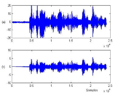
Figure 4. AVC output (bandwidth 0.1Hz) for a speech waveform. (a) Speech Waveform input to AVC
f
i(
t
)
(b) Output of AVC
f
o(
t
)
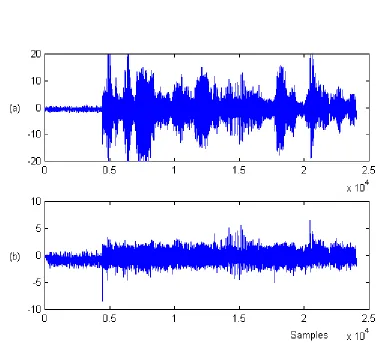
Figure 5. AVC output (10Hz bandwidth) for a speech waveform. (a) Original Speech Waveform
f
i(
t
)
(b) AVC Output
f
o(
t
)
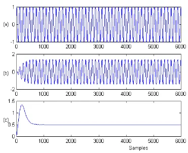
Figure 6 Variance Estimation for a sinusoidal input. (a) Signal Input to AVC
f
i(
t
)
(b) AVC Output
f
o(
t
)
(c) Variance Estimator Output
y
2(
t
)
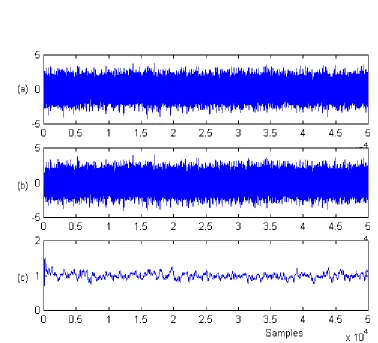
Figure 7. Variance estimation for white noise unit variance. (a) White Noise input to AVC
f
i(
t
)
(b) AVC Output
f
o(
t
)
(c) Variance Estimator Output
y
2(
t
)
Figure 8. Tracking the variance of a speech waveform. (a) Speech Waveform input to AVC
f
i(
t
)
(b) AVC Outputf
o(
t
)
(c) Variance Estimator Output
y
2(
t
)
6 Conclusions
7 References
[1] Haykin,S,” (1986) Adaptive filter theory”,Prentice Hall Englewood Cliffs,New Jersey
[2] Young, P.C. (1984) Recursive Estimation and Time Series Analysis: An Introduction. Springer Verlag: Berlin.
[3] Shan,T.J and Kailath,T, (1988), Adaptive algorithms with an automatic gain control feature, IEEE Transactions on Circuits & Systems, vol.35 no.1 ,pp122-127