Automatic indoor/outdoor scene classification

Rochester Institute of Technology

RIT Scholar Works

Theses

Thesis/Dissertation Collections

5-1-2002

Automatic indoor/outdoor scene classification

Navid Serrano

Follow this and additional works at:

http://scholarworks.rit.edu/theses

This Thesis is brought to you for free and open access by the Thesis/Dissertation Collections at RIT Scholar Works. It has been accepted for inclusion in Theses by an authorized administrator of RIT Scholar Works. For more information, please [email protected].

Recommended Citation

AUTOMATIC INDOOR/ OUTDOOR

SCENE CLASSIFICATION

by

Navid Serrano

A Thesis Submitted

In

Partial Fulfillment

of the

Requirements for the Degree of

MASTER OF SCIENCE

In

Electrical Engineering

Approved by:

Prof. Andreas E. Savakis, Thesis Advisor

Prof. Sohail

A.

Dianat. Thesis Committee

Prof. Raghuveer M. Rao, Thesis Committee

Dr. Jiebo Luo, Thesis Committee

Prof. Robert J. Bowman, Department Head

DEPARTMENT OF ELECTRICAL ENGINEERING

COLLEGE OF ENGINEERING

ROCHESTER INSTITUTE OF TECHNOLOGY

ROCHESTER, NEW YORK

AUTOMATIC INDOOR/OUTDOOR

SCENE CLASSIFICATION

I, Navid Serrano, hereby grant permission to the Wallace Library of the Rochester

Institute of Technology to reproduce my thesis in whole or in part. Any reproduction will

not be for commercial use or profit.

RochesterInstituteof

Technology

Thesis Abstract

AUTOMATIC

INDOOR/OUTDOOR

SCENE

CLASSIFICATION

By

Navid Serrano

Prof.Andreas E.

Savakis,

Chairperson ofthe

Supervisory

Committee

DepartmentofElectrical

Engineering

The advent and wide acceptance of digital

imaging

technology

has motivated an upsurge in research focused on _managing the _ever-growing number ofdigital images. Current research in

image manipulation represents a general shift in the field of computer vision from traditional image analysis based on low-level features (e.g. color and _texture) to semantic scene

understanding based on high-level features (e.g. grass and sky). One particular area of investigation is scene _{categorization,} where the organization of a large number of images is

treated as a classification problem.

Generally,

the classification _{involves mapping} a set of

traditional low-level features to _semantically meaningful _categories, such as indoor and outdoor

scenes,_usinga classifier engine. Successful indoor/outdoor scenecategorizationisbeneficialtoa number of image manipulation _{applications,} as indoor and outdoor scenes represent _among the

most general scene types. In content-based image retrieval, for example, a _{query for} a scene

containing a sunsetcanbe restricted to images in thedatabase pre-categorized as outdoor scenes.

Also,

inimageenhancement, categorizationof a scene as indoorvs. outdoor can leadtoimproved

color

balancing

andtonereproduction.

Prior research in scene classification has shown that high-level information can, in

fact,

be

inferred from low-level image features. Classification rates of_{roughly 90% have been} reported

using low-level features to predict indoor scenes vs. outdoor scenes.

However,

the high

classification rates are often achieved

by

_{using computationally} expensive, high-dimensional feature sets, thus

limiting

thepractical implementation ofsuchsystems. To addressthisproblem,

a lowcomplexity, low-dimensionalfeature set was extracted in a_variety ofconfigurations in the

work presented here. Due to their excellent generalization _performance, Support Vector Machines

(SVMs)

were used to manage the tradeoff between reduced

dimensionality

and

increased classification accuracy. It was determined that features extracted from image

subblocks, as opposed to the full

image,

can yield betterclassification rates when combined in a second stage. In particular, applying SVMs in two stages led toan indoor/outdoor classification

accuracy of90.2% on alarge database of consumer photographs provided

by

Kodak.

Finally,

it

TABLE

OF CONTENTS

1. INTRODUCTION 1

1.1 TheSceneClassificationProblem 1

1.2 Background 2

1.2.1 Scene ClassificationResearch 2

1.2.2 Indoor/OutdoorSceneClassification 3

1.2.3 FeatureExtraction 3

1.2.4 FeatureClassification 4

1.2.5 Feature Integration 4

1.3 ThesisContribution 6

1.4 Thesis Outline 6

2. LOW-LEVEL FEATURE EXTRACTION 7

2.1 ColorFeatures 7

2.1.1 LST Co/or Space 8

2. 1.2 LS7 Color Histograms 8

2.2 Wavelet Texture Features 9

2.2.1 Wavelet Transform 10

2.2.2 Wave/ef Basw Selection 13

2.2.3 Wave/e? Texture Feature Extraction 15

2.3 Edge Direction Features 16

2.3.1 Edge Detection 17

2.3.2 Edge MagnitudeandDirection 18

2.3.3 DominantEdge Selection 20

2.3.4 fi(ge Direction Histograms 20

3. LOW-LEVEL FEATURE CLASSIFICATION 21

3.1 Support Vector Machines 2 1

3.1.1 SVM

Training

21

3.2 Low-Level Feature SVM Training 24

3.2.1 Low-Level Features Extracted FromtheFullImage 24

3.2.2 Low-Level Features ExtractedFroma2x2 Tessellation 25 3.2.3 Low-LevelFeatures Extracted Froma4x4 Tessellation 26

3.3 InferringIndoor/OutdoorClassification From Subblocks 26

3.3.1

Majority

Classification 27

3.3.2 SynthesisofSubblockSVM Distances 29

3.3.3 Second Stage SVM 30

4. SEMANTIC FEATURE EXTRACTION 32

5. FEATUREINTEGRATION 34

5.1 Bayesian Networks 34

5.2 Indoor/Outdoor Feature Integration 37

6. RESULTS ANDDISCUSSION 39

6.1 ImageDatabase 39

6.2 Low-Level Feature Classification 39

6.2.1 Low-LevelFeaturesExtractedFromtheFull Image 39

6.2.3 Low-LevelFeatures Extracted Froma4x4Tessellation

4J

6.3 Inferring Indoor/OutdoorClassificationFromSubblocks 42 6.3.1

Majority

Classification

6.3.2 SynthesisofSubblockSVM Distances 6.3.3 Second Stage SVM

6.4 Feature IntegrationUsingaBayesian Network 4

6.4. 1 Bayesian Network FeatureIntegration

Using

Second Stage SVMresults 46

6.4.2 Full Bayesian Network FeatureIntegration 6.5 Computational Efficiency

42 44

45

7. CONCLUSIONS

8. REFERENCES

APPENDIX

50

51

52

1.

INTRODUCTION

1.1

The Scene Classification

Problem

The number ofdigital images to be processed, transmitted, and archived is

increasing

_rapidly as

the _quality and _variety ofdigital capture

technology

grow.

Consequently,

the need forefficient

digital imagemanagement

technology

hasalsorisenin importance. Aconcerted effortto

develop

technology

capable of

interpreting

the content of digital

imagery

has also gained momentum.

Successful interpretation of scene content _{i.e. image understanding} has been and remains a

very challenging problem in computer vision. It can be said that modern research in image

understandingevolvedfrom prior researchin imageanalysis [1].

However,

image understanding

deals primarily with high-level

(semantic)

scene information

including

people,

buildings,

and

natural _scenery, for example, while image analysis has

traditionally

focused on low-level image

content such as color andtexture.

Thus,

the challenge in image understanding has been to move

from low-level scenedescription tomoremeaningfulsemanticinterpretation.

An important area of research in image understanding is sceneclassification. The goal in scene

classification is to organize images categorically. Scene classification has been investigated

primarily for image database management applications.

Yet,

_any area

involving

image manipulation, such as digital photofinishing, stands to benefit from successful scene classification. Knowledge of the scene can

help

improve the performance of such digital

photofinishingoperationsas colorbalanceand_{tone reproduction,} for instance.

The inference of semantic scene content from low-level features has

traditionally

been

accomplished through statistical learning. Although this approach has been shown to be

successful, it does have limitations. The limitations rest, in particular, on the reliance on classifier engines to infer the semantic content from low-level features. High classification

accuracy can be achieved ifthere is _consistency between the images in the

training

set.

This,

however,

implies that theclassification will be less accurateforimages outside the

training

set

especially those with different scene characteristics. On the other

hand,

when large and diverse image sets are used to train the classifier _engines, the classification _accuracy also decreases

this is a _pervading challenge in the pattern recognition field in general, there are _encouraging

signs.

Specifically,

theincorporationofhigh-level scene informationtogether with thetraditional

low-level image featuresseems a _promisingapproachto sceneclassification.

1.2

Background

1.2.1

Scene

Classification

Research

Research in scene classification has been

largely

driven

by

applications

involving

the

manipulation of alarge volume of

imagery

[2].

Many

image database management systems have beenproposed overtheyears

including

QBIC

[3],

Photobook

[4],

VisualSEEk

[5],

NeTra

[6],

and MARS [7]. Most ofthese systems are example-based systems in thatthelow-level features of an

example _{query image} are used to find images in the database with similar features. These

low-level features generally include some formof color and texture image analysis.

However,

it is

well known that images with _{entirely different} semantic scene content can possess similar

low-level features. For example, it is entirely possible for a scene _containing a school bus to be

confused with a sunset scene _using color

features,

such as a color histogram.

Thus,

scene interpretation using low-level featuresaloneis usually ineffective. It is forthis reason thathigher level features have been investigated as a means of

improving

content-based image retrieval and imageunderstanding, ingeneral.

Theneedforautomaticsemantic sceneinterpretationand subsequent

indexing

in imagedatabases

werenotedin [4]. In

[8],

aparadigmfortextureannotation was_proposed, where a texturemodel derived from an image (or image region) is linked to a semantic

descriptor,

e.g. water. The inclusionof, for

instance,

shapeand sketch, as well astheirlocation and size was proposed in [3-7].

Yet,

image primitives

including

color, texture, and shape, to name a

few,

alone cannot

fully

bridge the _gap to semantic scene understanding. In

[6],

text annotations were used to describe

scene content. Although textannotationscan describesemantic scene content, thecontent canbe

varied, complex, andthus, subjecttointerpretation.

Furthermore,

the semantic description is not

automatic; it depends on human action. These

limitations,

as well as the _growing number of

research, where images _{are organized}

according to _semantically meaningful categories. Scene

classification _maybesupervised or unsupervised. In theunsupervisedcase, clusteringtechniques are usedto_{group images according}to theirsemantic scene content [9,10]. Inthe supervised _case, scenes are classified _usingpre-defined semantic_categories, e.g. indoorscenes vs. outdoor scenes.

1.2.2

Indoor/

Outdoor Scene Classification

Because,

in general, scene classification is challenging, the problem can be simplified

by

considering broad scene _categories, such as indoor scenes vs. outdoor scenes.

Clearly,

other semantic categories could beexplored _and, in

fact,

categorization _according tohuman preference

has been investigated [11].

However,

indoor/outdoor classification has received significant

attention _partially because of its importance in image enhancement, as discussed earlier. Szummer andPicardfirstexploredindoor/outdoorsceneclassification andshowed thathigh-level image content could be deduced through statistical classification of low-level image attributes [12]. Laterresearch_{addressing indoor/outdoor}classification includesthework ofPaeketal

[13],

Vailaya et al

[11,14],

Savakis and Luo

[15],

and Guerin-Dugue and Oliva

[16],

toname a few.

Althoughtheseapproaches_varyin_{manyrespects,} some generaltrendscan be discerned.

1.2.3

Feature Extraction

Almost all documented indoor/outdoor scene classification work involves some degree of

low-level feature extraction. In general, indoor/outdoor classification approaches _{employ color,}

texture, and to a lesserextent, spatial

frequency

low-level features. These features are

typically

computed oneither theentire image orimage subblocks. The most common colorfeaturesused for indoor/outdoor classification include colorhistograms

[12,13,15]

and color moments [11,14]. In terms of texture

features,

the Multiresolution Simultaneous Auto-Regressive

(MSAR)

model

was explored in

[11,12,14,15],

edge direction histograms were considered in

[11,13,14],

and Local Dominant Orientation

(LDO)

distributions were used in [16]. Spectral

features,

such as discrete cosine transform

(DCT)

coefficients, have alsobeen

investigated,

though

they

have been

image,

whereas the other approaches in

[11-14]

extract the features from image subblocks.

Finally,

in

[13],

textual features are derived from text annotations and combined with

image-based featuresfor

indoor/outdoor

classification.

1.2.4

Feature Classification

It can be said that there are two

dominating

paradigms for the classification of low-level

indoor/outdoor image features:

1)

featureextraction andclassificationfrom image subblocks,and

2)

feature extraction and classification from the full image. If the first approach is used, the

subblock features can be concatenated in order to obtain a feature vector _representing the full

image,

as in [11,14,17]. Classification oftheconcatenatedfeature vectorthenyields afull image

indoor/outdoor label.

Alternatively,

the subblock features can be classified

independently

[12].

This implies that the _{resulting indoor/outdoor} classification foreach subblock must somehow be

combined toproduce an indoor/outdoor label corresponding to the full image. The second, less

common, approach, as in

[15,16],

involves low-level feature extraction and subsequent feature

extraction fromthewhole image.

In terms of specific classifier engines, the ^-nearest neighbor

(&-NN)

classifier has been

frequently

used and shown to produce favorable results for indoor/outdoor classification

[12,15,16]. The main

drawback, however,

is that &-NN classifiers are _generally slow. A more

efficient Bayesian classification approach was used in

[11,14]

to _classify concatenated subblock

features.

However,

concatenatedfeature vectors canbe very high dimensional. Not _{surprisingly,}

the concatenated feature vectors used in

[11,14]

had on the order of 600 dimensions. High

feature

dimensionality

can beproblematicandis

typically

avoided.

1

.2.5

Feature Integration

The indoor/outdoor classification methods described in

[11,14,16]

construct a feature vector

correspondingto theentire image. The final indoor/outdoorassignment is produced

by

statistical

relationship between the

low-level

features and the semantic scene content. Approaches ofthis type have

typically

achieved indoor/outdoor classification rates _slightly lower than 90%.

Specifically,

in

[11,14],

indoor/outdoor

classification rates of88.2% and88.7% werereportedfor

two independent image test sets. The work described in

[16]

included two other classes {open

andclosed_scenes) in additionto theindoorand outdoor classes_{resulting in}anoverall recognition

rate of88.7%.

Many

oftheother referenced approaches involveadditional feature integration (or

interpretation)

before _making a final indoor/outdoor_category assignment. In

[12],

two distinct classifiers were trained for color and texture features extracted from a 4 x 4 image tessellation.

Consequently,

two indoor/outdoor labels are assigned to each image subblock one _{resulting from} the color classifier and another from the texture classifier. The final indoor/outdoor classification was decided

by

_majority vote. Afinal indoor/outdoor classification rate of90.3% was reported on a

databaseof 1324 images provided

by

Kodak.

However,

in

[13]

this method was evaluatedon a

distinct image database of 1300 news images and the indoor/outdoor classification rate dropped to74.7% _{significantly lower}than 90.3%. This

drop

couldbe dueto thefactthatKodak's image database contains a large number of images with duplicate scene content that might inflate the

classification rates. This issue isrevisited insection6.1.

Otherapproaches have integrated the low-level image features described in the previous section with higher level features. For

instance,

Paeket al

[13]

proposed a unique approach tointegrate low-level color and texture features computed over image subblocks together with textual

informationaboutthecontent ofthescene.

Using

this technique, anindoor/outdoorclassification rate of86% was reportedon adatabase of_{approximately 1300}news images.

In

[15],

SavakisandLuo computed colorand texture features analogous to [12]. As in

[12],

a

k-NN classifier was trained for both the color and texture features.

However,

the features were computed over the entire

image,

rather than image subblocks.

Using

this _approach,

indoor/outdoor classification rates of74.2% and 82.2% were obtained for the color and texture

features,

respectively, on the Kodak image database (minus 15 ambiguous _scenes) used in [12].

They

also proposed a paradigm for the integration of the low-level color and texture features

Bayes net was used to

integrate

the indoor/outdoor beliefs obtained _using color and texture

featurestogetherwithsemantic

information

thatdistinguishes outdoor scenes fromindoorscenes,

such as the presence of grass and/or _sky regions in an image. This approach yielded a final

indoor/outdoor

classification rate of 90.1% _using grass and _sky ground truth and _{84.7% using}

computed grass and _skyfeatures.

1.3

Thesis Contribution

The work presented in this thesis proposes an improved approach to indoor/outdoor scene

classification. The

key

contributions ofthis thesisare thefollowing:

1)

Low

dimensional,

_{low complexity feature}set

2)

Application ofSupport Vector Machines

(SVMs)

tolow-level featureclassification

3)

ApplicationofSVMstointerpretsubblockbeliefs ina second classification stage

4)

Increased overall indoor/outdoor classification

by integrating

low-level and semantic

features_usingaBayesiannetwork

1.4

Thesis

Outline

The thesis is organized as follows. Section 2 introduces the low-level feature set tobe used for

indoor/outdoor classification: color

histograms,

wavelet coefficients, and edge direction histograms. Section 3 discusses low-level feature classification _{using SVMs. In addition,} a

variety of configurations for feature extraction and classification are proposed. Section 4 describes the use of semantic feature detectors for indoor/outdoor classification. Section 5

presents an introduction to Bayesian beliefnetworks and a paradigm for the integration of

low-level and semantic features for indoor/outdoor classification. Section 6 delineates the results

fromeach approach and compares the classification _accuracy oftheproposed systemto _existing

2.

LOW-LEVEL

FEATURE EXTRACTION

This sectiondescribes a series oflow-level features for indoor/outdoor classification. Color and

texture attributes constitute the most common low-level features in scene classification.

Many

color and texture analysis _{techniques exist,} and a number of these have been proposed for

indoor/outdoor classification. Popular color features include color moments

[11,14,17],

color

histograms

[12,15],

color coherence vectors

[11,14,17],

and color correlograms [18]. Popular

texture

features

include MSAR features

[11,13,14,15,17],

edge direction histograms

[11,14,17],

edgedirectioncoherence vectors

[11,14,17],

andLDO distributions [16]. Althoughthesefeatures

have been shown tobe effective for indoor/outdoor _{classification,} prior research has focused on

successful resolution of the indoor/outdoor classification problem

first,

and

tractability

second.

Hence,

the low-level features considered here were assessed not _only in terms of their

effectivenessfor indoor/outdoorclassificationbut also in terms oftheircomputationalefficiency.

Three different low-levelfeatures were evaluated: color

histograms,

wavelettexture

features,

and

edge-directionhistograms.

2.1

Color Features

It is well known that the spectral characteristics of natural and artificial illuminants can _vary

considerably [19].

Moreover,

the primary light source in a scene will impact the color

reproductionin a_photograph, be it digital or analog.

Thus,

illuminant differences are _among the

most important scene characteristics that distinguish indoor scenes from outdoor scenes.

Reconstruction of the spectral characteristics of the illumination source in a scene remains a

difficultproblem

[20]

andtherefore, beyondthescope ofsceneclassification.

Instead,

thegoal in

indoor/outdoorclassification is to capture coarse scene illumination differences

by

_using simple,

well-established color features. Color histograms were used in the indoor/outdoor classification

system proposed here because of their simplicity. Based on prior use of color _{histograms for}

indoor/outdoorclassification

[12,15],

theprecision ofthe histograms was reduced

by

afactorof2

inordertoimprove efficiency. Thechoice of color spaceis of prime

importance

andis addressed

2.1.1

LST Color Sp,

ace

Many

factors impact the selection of a color space. These factors _{may include} the statistical distribution of color _{signals, the} effect of noise in color _{coordinates, the} effect of light source

variations, and theeffect of reflectance variations. Basedon these considerations, the LSTcolor

space, also knownasthe Ohta color space orT-space

[21],

isa goodchoice. The LSTcolorspace

has beenshown tobeusefulinimage_processingapplications

[22]

andis detailed below:

Foran8-bit

image,

oris givenby:

L= -^=-(R+G+

B)

(1)

V3

S=-^=.(R-B)

(2)

V2

T=-%=(R-2G

+

B)

(3)

V6

255

d=

? r

(4)

Max{R,G,B

}

The three LST components are orthogonal and have unit length. The LST color space is a

luminance-chrominance representation and the color components are _{thus, approximately}

decorrelated. The ST

(chrominance)

components are

intensity-invariant,

_meaning

they

do not

vary with light source

intensity

changes.

Furthermore,

the S component ofthe LSTcolor space

represents daylight to tungsten illuminant variations.

Finally,

LSTcolor channels represent the

principalcomponents of a largeselectionof naturalRGBimages.

2. 1

.2

LST Color Histograms

Having

transformedaninput RGB image to theLSTcolor_space, colorhistograms foreach ofthe

L, S,

andT channels, _{respectively.}

Where,

b=l,2,...,nc

_{representsthe}

gray level

bins,

and_nc isthe

total number ofbinsper colorhistogram. Theconcatenated

L,

S,

and Thistograms constitutethe

colorfeature vector xc:

xc =

[hL(l), hL(2),...,

hL(nc), hs(l), hs(2),..., hs(nc), h^l), M2),...,

h-fa)]

(5)

This color feature approach is analogous to that of

[12,15]

(including

the choice ofcolor space).

The

dimensionality

ofthe colorhistogram feature vectoris equalto 2>nc. Thenumber ofbins per

color histogram was set to c=16 for a feature

dimensionality

of 48. In

[12,15],

32 bins per

histogram were used for a feature

dimensionality

of96.

Therefore,

the color features proposed

herehave halfthe

dimensionality

oftheanalogousfeatures usedin [12,15].

2.2

Wavelet Texture Features

Texture has

long

been an area of research in image analysis. The numerous texture features

proposed over the years can be divided into five categories [23]: _{statistical, geometrical,}

structural, model-based, and signal _{processing features.}

Early

approaches to texture analysis

relied _mostly on statistical features [24,25]. It has since been shown,

however,

that statistical

methods do not _{adequately describe both local} and global textural information [26]. Attention

has thus concentrated on signal _processing approaches, and in _particular, multiresolution

methods, which better preserve both local and global information [27,28]. Ofparticular note is

theaforementionedMSAR model introduced

by

MaoandJain [29]. As noted _{earlier, the}MSAR

model has been used _{considerably for indoor/outdoor} classification [11,12,14,15,17]. Despite

their popularity, MSAR texturefeatures are _{computationally intensive.} A more _{computationally}

efficient alternativeis thewavelettransform[30].

The last

decade,

especially, has produced a host of work on the wavelet transform and its

applications. Not originallyenvisagedas atool fortextureanalysisper_se, the_{applicability}ofthe

wavelet transform to texture analysis was first proposed in the _pioneering work of Mallat [31].

Wavelet packets (or tree-structured wavelet

transform)

[32],

and wavelet

frames

(or

wavelet

features

performed

favorably

compared to other signal _processing texture

features,

including

MSAR

features,

in a recent evaluation [34]. Beyond texture analysis, the use of the

wavelettransformhas beenextendedtohigh-level scene_analysis,as surveyed in [35].

Finally,

it is worth _noting that the wavelet transform has also been shown to exist in biological visual

systems [36]. Due to their comparative computational _efficiency and positive performance in

texture analysis, waveletfeaturesare consideredhere.

2.2.1

Wavelet

Transform

Multiresolution analysis

(MRA)

refers to theprocess of

decomposing

a signal intoa

hierarchy

of

approximation and detail coefficients. Fundamental to MRA is the fact that the original signal

can be reconstructed _{perfectly from} the approximation and detail functions if the proper

methodology is employed. _{Simple scaling} alone is notfeasible because

frequency

information is

lost,

thus_{making it impossible} toreconstruct theoriginal signal exactly.

However,

ifthe _scaling

is preceded

by

a

filtering

stage_using alow-pass

(LP)

filter

h0(n)

and a high-pass

(HP)

filter

hx(n),

the original signal can bereconstructed_perfectly

by

_scalingthe analyzed signal andthen

filtering

itwitha LPfilterg0(n)and a HPfilterg\(n). Thedecompositioncan be done multiple times thus

producingmultiple scaled versions oftheoriginalsignal the aforementionedhierarchy.

The wavelet transform is a specialized formof

MRA,

where the signal is decomposed into a set

offunctions i/fm,n(t) defined by:

Vm,n(t)=

2m/2y/(2mt-n)

(6)

The

family

of functions ofEq.

(5)

is generated

by

translating

and

dilating

the mother wavelet

y/(f). The mother wavelet satisfies

\yAf)dt=Q,

and is constructed from a _{scaling function (fit)}

accordingto:

V(0=

^h\(kM2t-k)

(8)

k=-Where,

h0(k)

and

hx{k)

are the coefficients of the aforementioned LP and HP decomposition

filters,

respectively. If a discrete wavelet transform

(DWT)

is used, the filter coefficients

themselves can be used instead ofthe continuous functions yAt) and <p(J). Biorthogonal wavelet

filter banks are a special class of DWT. In a biorthogonal wavelet representation, the

decomposition filters

h0(n)

and

hx{n)

_satisfyand are relatedby:

5>o()

=i

(9)

n

2(-l)"-1/z1(n)

=2

(10)

n

hl(n)

=

(-l)nh0(l-n)

(11)

Thereconstruction filters_g0(n) and_gi(n)are relatedto

ho(n)

and

h^n)

_accordingto:

g0(n)=

(.-iyhl(l-n)

(12)

g1(n)=

(-l)n-1ft0(l-)

(13)

The biorthogonal denomination stems fromthefact that

h0(n)

and_g\(n) are _mutuallyorthogonal

as are

h{(n)

andgo(n). In_addition,biorthogonal filter banks are symmetric (i.e. have linear phase)

and are_{approximately decorrelated.}

The 2-D DWT is an extension of the 1-D case. In

fact,

a separable 2-D DWT can be _easily

implemented

by

_applying the 1-D filters (described _{above) along} the two

dimensions

of the

signal. For a given image

f\x,y),

a one-level, 2-D separable DWT decomposition can be

implemented

by

_convolving therows and columns of

J\x,y)

with combinations of

h0(n)

and

hx(n),

oo oo

LLX

(x,

v)=

X S

/(*.

J)K

d

-i*)h

U

-2y)

(=-;

LHl(x,y)=

J

JJf(i,j)h0(i-2x)hxU-2y)

HLl(x,y)=^^jf(i,j)hl(i-2x)h0U-2y)

i=-~j=-////1(^y)=XS/0".M0-2^O'-2y)

(14)

(15)

(16)

(17)

Where, LL,

LH,

HL andHH stand for

low-low, low-high, high-low,

and

high-high,

respectively.

Specifically, LLx{x,y)

represent the approximation coefficients and

LH:(x,y), HL\(x,y),

and

HHi(x,y)

representthedetail coefficients. The subscriptdenotes the decompositionlevel (in this

case 1). Figure 1 showsthe2-DseparableDWT implementationgraphically.

M/2xN/2

MxN

rows

TJ-^N^)

columns

^TT-(jg)-

LL!

ft!

4-2

HL,

aTT-(^2)

columns

>

/fa

H4-2

LH,

[image:18.613.108.496.399.590.2]

>

A?

_-H4-2

HH,

Figure 1. 2-DseparableDWT implementation.

Wavelet coefficients are

typically

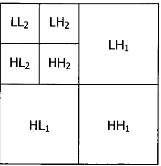
depicted using the pyramid structure shown in Figure 2. As

can be seen from Figure

2,

for each level of

decomposition,

it is the

low-frequency

coefficients

that are furtherdecomposed. This implies that the final decomposition at level Kwill consistof

one coarse approximation (the final

low-frequency

_{coefficients)} and K sets of detail (high

LL2

LH2

LH!

HL2

HH2

[image:19.613.230.389.90.253.2]

HL!

HHi

Figure 2. Two-levelpyramidDWTstructure.

2.2.2

Wavelet Basis Selection

Animportantpoint ofconsideration when_employingthe DWTis theselection of a wavelet basis

(i.e. filter bank).

Many

wavelet filter banks exist, each _possessing distinct properties.

Biorthogonal wavelets(discussed intheprevious _section)have been shown tobe useful for image

compression

[37]

andwill be used in the newJPEG2000compression standard [38]. In the area

of texture analysis,

however,

no formal evaluation of wavelet filter banks had been conducted

until recently.

Daubechies'

filter banks have

traditionally

been a popular choice for wavelet

texture analysis [32,39,40,41].

Yet,

the selection of a wavelet basis for texture analysis has

largely

been subjective or arbitrary. In

[42],

Mojsilovic et _al, attempt to define an optimal

wavelet basis for texture characterization. Their study _showed,

first,

that the selection of

decomposition filters _notably impacts texture characterization.

Second,

in _comparing 19

orthogonal and biorthogonal wavelet

filters,

they

found that biorthogonal filters outperformed

orthogonal filters. A simple _{study described below} provides further motivation for the use of

biorthogonal,

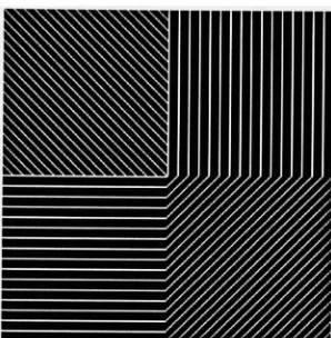
as opposedto, orthogonalfilters.

A simple test imagewith edges oriented in four directions

(0, 45,

90,

and 135

degrees)

is shown

in Figure 3. The edges in the image have a width of one pixel. The simple test involves a

waveletdecompositionofthe testimage using

Daubechies'

popular

4-tap

orthonormalfilter

(db4)

andthe5/3 biorthogonal filter(bior5/3). The

LHX

and

HLX

waveletcoefficients _{corresponding} to

corresponding

to the

bior5/3 decomposition

_{are shownin Figure4b. As canbe seen fromFigure}

4a,

an

interesting

_{artifact appears}

when _using the db4 filter.

Namely,

the db4 filter is unable to

properly extract the edges oriented at 135 degrees (the first quadrant inthe test

image),

whereas

the

bior5/3

filters does. This is relatedto the

frequency

response ofthedb4 filterand is _clearly,

anundesirableresult.

Figure3. Edgepattern usedforwaveletfilterevaluation.

[image:20.614.250.399.215.367.2]

(a)

(b)

Figure 4.

LHX

and

HLX

coefficients_usingthedb4 filter

(a)

andthe_{bior5/3 filter}(b).

Another consideration is computational efficiency. _{Shorter filter lengths}

are, obviously, more

computationally efficient as

they

requirefewernumerical operationsper pixel.

Considering

both

computational

tractability

and optimal texture _{characterization,} the

bior5/3

wavelet filters were

selectedfortheproposedindoor/outdoorclassification system.

Finally,

the

bior5/3

filter is one of [image:20.614.87.562.469.600.2]

filter may provide

further

_efficiency gains when the indoor/outdoor classification system is

implemented

in conjunction with the JPEG2000 codec. The bior5/3 decomposition filters

h0(n)

and

hi(n)

are shown in Eq.

(18)

and (19). In this case

they

are not shown in normalized form in

orderto

illustrate

thefactthat

they

areintegercoefficients.

h0(n)

=

[-l

₂ 6

2-1]

hx(n)

=_{[l -2}

1]

(18)

(19)

2.2.3

Wavelet

Texture Feature Extraction

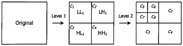
Let c2, cs, c4, c5, c6, c7, and _cs represent the subband coefficients of the two-level wavelet

decompositionas shownin Figure 5.

Level 1 Ci

LL! LHi

Cs

HLi

C, HHi

Level2

CS C6 C2 c? Cs

[image:21.613.151.455.381.458.2]

c3 c*

Figure 5. Coefficient labels forwavelettexturefeatureextraction.

As can be seen from Figure

5,

c2=LHl(x,y), c3=//L1(x,y), cA=HHx{x,y), c5=LL2(x,y), c6=LH2(x,y),

c7=HL2(x,y),andc&=HH2(x,y). Coefficientset_c5 isa

low-frequency

approximation ofthe original

signal. The other coefficients provide

directionally

correlated measures of the

high-frequency

signal content. Because natural textures contain _mostly mid to high

frequency

information,

the

low-frequency

coefficients are not

inherently

useful for texture description.

Thus,

rather than

using the raw

LLiix,y)

wavelet coefficients, set _c5 is redefined

by filtering

LL2(x,y)

with the

Laplacian filter:

M N

c5=YjYj LL2

G'

Ml

(*

~

,y~

J)

.=1 ;=1

Where,

MandNarethe

dimensions

of

LL^y)

and

hL{x,y)

istheLaplacian filter:

hL(x,y)

=

-1 -1 -f -1 8 -1 -1 -1 -1

(21)

Because the Laplacian filter provides an isotropic measure of the

high-frequency

signal

information,

the filtered coefficient set _c5 can be regarded as a measure ofnon-directional high

frequency

energy in the image.

Ultimately,

the texture features are obtained

by

_computing the

subband _{energy for} all wavelet coefficients

(including

the Laplacian filtered c5 coefficients)

accordingto the

following

general expression:

M N

ek

1 M _"_

= _k=2,X..AK

(22)

Where,

M and N are the image dimensions of coefficient _ck, and K is the number of decomposition levels (in this case 2).

Therefore,

seven wavelet texture features are obtained. This represents a reduction

by

a factor of 2 compared to the 15 MSAR features used in

[11,12,14,15,17]. Thewavelet texturefeature vectorx,is definedas:

\,=

[e2,e3,...,e8]

(23)

2.3

Edge Direction Features

It has been observed that _many types of scenes have directional edge signatures. For

instance,

scenes _containing man-made structures (e.g. city _scenes) tend to have edges with dominant orientations. On the other

hand,

images with a predominance of natural _scenery (e.g. landscape

scenes) tend to havemorerandomlyoriented edge content.

Hence,

it is reasonabletoassume that

directional edge features might be _{strong discriminators} between certain types of scenes. Not

for

indoor/outdoor

classification in [9,12,13]. Other

directionally

sensitive features have also

been used for

indoor/outdoor

_{classification,}

including

_{the LDO distributions introduced in [16].}

In

keeping

with the goal of computational efficiency, edge direction histograms are considered

here.

The process involves four basic steps:

1)

edge

detection,

2)

computation of the edge magnitude

and

direction,

and

3)

selection of dominant edges, and

4)

construction of the edge direction

histogram. The method of Lee and Cok

[43],

which provides a framework for

detecting

boundaries in color images and _estimating their magnitude and

direction,

is adopted here and

summarizedbelow.

2.3.1

Edge Detection

Given an image

j\x,y)

with three color attributes

(R,G,B),

the individual color planes can be

definedas:

r(x,y)=fix,y) e R

(24)

g(x,y)=fix,y) e G

(25)

b(x,y)

=f{x,y) G B

(26)

The horizontal edges can be obtained

by

_convolving each of the above color planes with a

derivative filter

hx(x,y),

thus_yieldingthepartialderivatives:

-\ M N

^-

=

yYr(i,j)hx(x-i,y-j)

(27)

MM

-\ M N

7T

=

EE

*<'*<*-'>-./)

(28)

dx _/=1 ;=1

M N

Where,

M and N

denote

the row and column dimensions ofJ\x,y).

Similarly,

the vertical edges

are obtained

by

convolving

the color planes with aderivative filter hy(x,y):

^_ m N

,

=J\Y,r(i,j)h

(x-i,y-j)

M N

-r-=

y,J\

s(*.

My

(*

-*.y

-J)

y

ri%

db M N

V=

EE

W*

My

(x

-i,y-j)

y _mm

(30)

(31)

(32)

The filters

hx(x,y)

and

hy{x,y)

can _{be any derivative filters. The} well-known Prewitt filters were

used

here,

where:

hx(x,y)

-1 -1

0 0 0

1 1 1

(33)

K(x,y)

=

-1 0 1

"

-1 0 1

-1 0 1

(34)

Finally,

itshould be noted that theimage

f\x,y)

wasfirst smoothed _usinga Gaussian filter before

applying filters

(33)

and

(34)

inordertosuppresstheeffect of spurious edges.

2.3.2

Edge Magnitude

and

Direction

Having

estimatedthehorizontal and vertical _edges, a matrixD composed ofthepartial derivative

~dr

dx

_oy

og

dg

dx

_oy

db

db

dx

oy\

D= Z*. ^

(35)

The edge magnitude and direction can be obtained from principal component analysis of the

matrix product

DTD,

where the largest eigenvalue corresponds to the edge magnitude. The

largesteigenvalue

X

andthustheedge magnitudeis givenby:

X

= 2L

a+b+yl(a+

b)2

-4(ab-c2)

(36)

Where,

+

fdg}2 fdb^2

\0XJ

+

KdXj

/3^2

/aV /a^^2

b=

dr_

₊

dg_

oy)

+ db

_

dr dr

dg dg

db db

dx

dy

dx

dy

dx

dy

(37)

(38)

(39)

The eigenvector _{corresponding} to the largest eigenvalue

X

provides the edge

direction,

which in

turn can be used to compute the edge angle. The partial derivatives

dr/dx, dr/dx, db/dx, drldy,

dgldy,

and

dbldy

havevalues associated with all points in f{x,y).

Thus,

each pixel location inthe

2.3.3

Dominant Edge

Selection

It is not meaningful to construct an edge direction histogram without first _analyzing the edge

magnitude and

determining

_{whether or not it is} a dominant (i.e. significant) edge.

Canny'

s

popular edge detector

[44]

can be used for this purpose. Candidate points are those that arethe

local edge magnitude maxima _along the _{corresponding} edge direction. A candidate point is

regarded as an edgeifits edge magnitudeisgreaterthanalowthreshold

T,

and isconnectedtoat

leastone pointthathasan edge magnitude greaterthanahighthreshold T2. Thethresholds

Tj

and

T2

are

typically

determined _empirically

depending

onthedesired degreeof edge selectivity.

2.3.4

Edge Direction

Histograms

An edge direction histogram is accumulated_{only for} those points that were marked as dominant

edges _according to thecriteria ofsection2.3.3. Let

he{b)

be theedge direction

histogram,

where,

b-l,2,...,ne

represents theedge direction bin _element, and_ne is the totalnumber ofbins per edge

direction histogram. In other _{words, ne} defines the number of edge angles to include in the

histogramhe. Theedgedirection featurevector_\eisgiven by:

xe=

[he(l),he(2),...,he(ne),MN-^he(b)]

(40)

b

The last element in the feature vector (which is not part of the edge direction

histogram)

representsthenumberofnon-edgepoints, whereMandNarethe row and columndimensions of

the imageor imagesubblock. The

dimensionality

oftheedgedirection histogram isne + 1. The

numberofbins per edgedirection histogramwas set_{to ne=36,} forafeature

dimensionality

of37.

Thisis _{roughly half}the

dimensionality

ofthe analogous edge direction histograms of

[11,14,17],

where 5

3.

LOW-LEVEL FEATURE CLASSIFICATION

3.1

Support

Vector Machines

The Support Vector Machine

(SVM) [45,46]

is a new method of parameterization of

functions,

and therefore has application outside the realm of predictive learning. It has been called a

universal

learning

procedure because it can be used to learn various representations such as

neural _networks, radial basis functions

(RBF),

polynomial _estimators, etc. In the pattern

recognition _context, SVMs have been used for

handwriting

recognition

[47],

text categorization

[48],

and face detection [49]. SVMs have been shown tohave equivalent or _{significantly better}

error rates than comparative classification methods [45]. One characteristic, in particular,

separates SVMs fromother classification paradigms optimization ofthe _{separating hyperplane.}

This optimization (discussed in the

following

_section) results in better generalization beyondthe

training

dataset. Forthesereasons, SVMswere usedin the indoor/outdoorclassification scheme

proposedhere.

3.1.1

S

VTS/L

Training

In preceding sections, a colorfeature vectorxc, a wavelettexture featurex,, andanedge direction

feature vector _xe were introduced. A general feature vector x will be used in this section for

discussion purposes only. It should be noted that the discussion applies _equally to the feature

vectors_{xc, x} andxe.

Supposethere are/observationsdescribed

by

a feature vector_x, s

Rd,

i=l,...,l and the associated

truth y, e {-1,1 } Ifobservation icorresponds to an outdoor

image,

_{then y,=l,} otherwise y,=-l.

The objective is to find some _way of _separating the observations such that there is a clear

distinction betweenthetwoclasses_y, (i.e. indoor vs. outdoor). Thereare

infinitely

_many ways of

separating the

data,

however,

the separation that yields the best generalization performance is

desired. To illustrate this

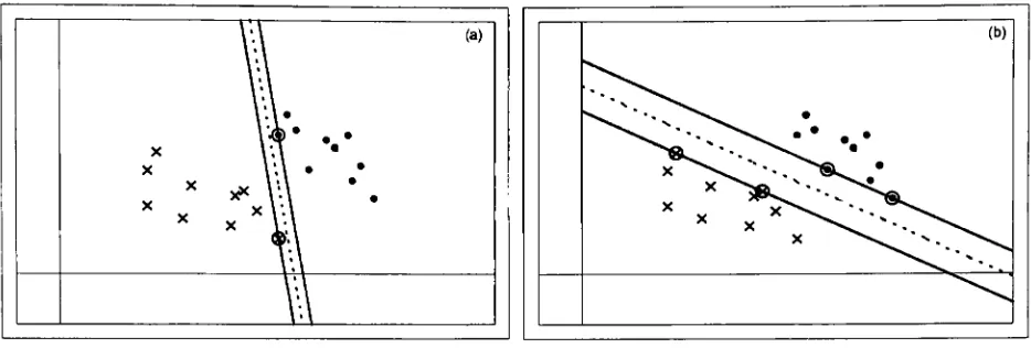
further,

a simple linear classification is shown in Figure 6. Figure 6a

depicts a successful separation ofthe

data,

with minimal _margin, where themargin is the sum of

the perpendicular distances from the closest point of each class to the _{separating hyperplane.}

Intuitively,

the case in Figure 6b will have better generalization performance (lower [image:28.613.73.540.148.306.2]

generalization error).

Figure 6. Successful SVM linearclassification with sub-optimal _(a)andoptimal _(b)margins.

Forthelinear-separablecase shownin Figure

6,

thehyperplane thatseparatesthedatasatisfies

w x+b=0

(41)

Where,

w is normal to the

hyperplane,

and

|b|/|w|

is the perpendicular distance from the

hyperplane to the origin. The parameters, w and

b,

are determined

by

training

the SVM. The

optimalhyperplaneis obtained

by

_maximizingthe marginsubjectto theconstraints

Xj- w + b> +1, fory,=+1

Xi w +b>-1,fory,=-1

(42)

(43)

which canbecombinedinto

y,(x, w +

b)

-1 >

0,

_Vi

(44)

All points that _satisfy

(42)

lie on thehyperplane H,: _x, w + b= 1.

Points satisfying

(43)

lie on

the hyperplane H2: x,; w + b =-1. Hyperplanes

Hj

and

H2

are shown in Figure6 as solid lines.

are the points with an additional circle. The perpendicular distance from both

H,

and

H2

to the

shattering hyperplane

(41)

is

l/||w||,

and _thus,themargin is_{simply 2/||w||.}

As stated _{earlier, the} goal is to maximize the margin

during

SVM training. This optimization

problem canbesolved _{using Lagrange}multipliers. Thefullderivation _{is elegantly laid}outin

[43,

44]. Forthesake of

brevity,

_onlythesolutionisnoted below:

/(x)

=

JA,7;xrx,.

_+b

(45)

i=\

Where,

A,

are the Lagrange multipliers. As can be seen, equation

(45)

is a function of the

observation (or

feature)

vector, x, and can be interpreted as thedistance (in feature space) ofthe

point x fromthe _separating

hyperplane,

ordecisionsurface(41).

Up

tothis point, onlythe

linear,

separable SVMcase has beentreated. A solution similarto

(45)

can be obtained for a non-linear SVM using a kernelfunction K(x,Xi). The reader is again

referred to

[14,

19]

for full derivations. Thenon-linearSVMsolution is:

f(x)

=

^XiyiK(x,xi)

₊b

(46)

i=i

Clearly,

Eq.

(46)

is similar in formto Eq.

(45)

and in

fact,

can be said to encompass the linear

case, where

A"(x,x,)

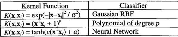
= _xTx,. Somecommon kernel functions fornon-linearclassification are listed [image:29.613.157.455.629.692.2]

in Table 1.

Table 1. Possible SVM kernelfunctionsandtypeof classifier.

Kernel Function Classifier

/C(x,x,)

=_{exp(-|x-x,|2/a2)} Gaussian RBF

K(x,x.)

= (xTx,-₊

If

Polynomial ofdegreep

K(x,Xi)

=_tanh(v(x'x/) +a) NeuralNetwork

Attention is now given to the non-separable data case. Most real life problems are of the

decision surface without some misclassification.

Furthermore,

when faced with the non-separable case, the above equations have no solution. To obtain a feasible solution forthe non-separable case and to manage the tradeoffbetween the margin and misclassification, constraints

(42)

and

(43)

(forthelinear_case),are relaxed asfollows:

xrw + b>_+1-4, fory,=+1

(47)

x, w+ b>

-l+, fory,=-1

(48)

&>0Vi

(49)

For an error to occur , must exceed _unity and

hence, ,

is an upper bound on the number of

training

errors. Acost parameter C is then

introduced,

where C>

0,

such that the function to be

minimized changesfrom

||w||2/2

to

||w||2/2

+CZ,. The optimizationproblemcan againbe solved withLagrange multipliers, where0<X,< C. Thecost parameter is determined before

training

by

the user; alarger Ccorrespondstoahigher penalty forerrors. A similarapproach is used forthe

non-linear SVM. For a more complete description of the solutions

incorporating

the cost parameter

C,

thereaderis again referredto [45,46].

3.2

Low-Level Feature SVM

Training

An RBF kernel (see Table

1)

was used to train the color, texture, and edge direction features

separately. The choice of kernel was arbitrary. The SVMs were trained _using the "SVMfu"

algorithm developed at MIT's Artificial Intelligence Lab [50]. The SVMs were trained _using low-level features extracted from the full

image,

as well as image subblocks from a 2 x 2

tessellation and a 4 x 4 tessellation. In each _{case, the} feature vectors were normalized to zero mean and unitvariancebeforetraining.

3.2.1

Low-Level Features Extracted From

the

Full Image

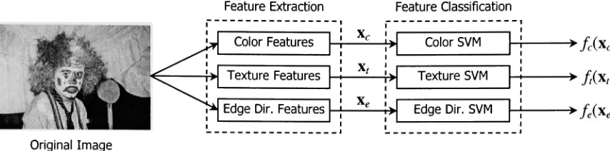
In this configuration, the color, texture, and edge direction feature vectors _{xc, x} and _xe

distance measures

/c(xc), /,(x,),

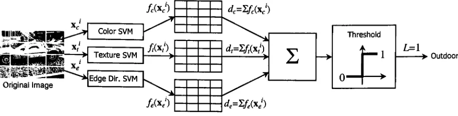
_{and/e(xe) respectively,} which represent the indoor/outdoorbeliefs

fortheimage in question. Theprocessisshown _{schematically in Figure 7.}

FeatureExtraction Feature Classification

ColorFeatures

Texture Features

Edge Dir. Features

Color SVM

TextureSVM

Edge Dir. SVM

-?/c(xc)

+

ffa)

+M*e)

Original Image

Figure7. Low-level featureextraction and classificationfromthefull image.

3.2.2

Low-Level

Features

Extracted From

a

2

x

2

Tessellation

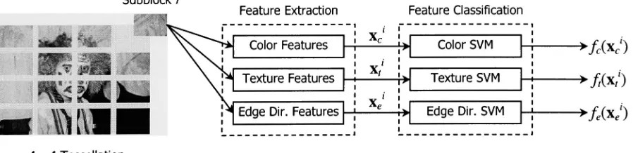
In this case, the image is divided into 4 subblocks. For a given M x Nresolution

image,

each

subblocks willbe of sizeMI2 xN/2. Let i=l,2,...,4 denotethesubblocks of a source image. The

feature vectorsxc', xj, and_xj are extractedfromeach subblocki and classified separately. SVM

distancemeasures

fc(xc'),f,(x,'),

_and/e(x,')are_thus,also obtainedforeach subblocki.

Feature extraction from image subblocks can be expected to achieve less _accuracy compared to

the full image

features,

as there are fewer and weaker signatures. Although less accurate,

subblock classification offers further alternatives to

inferring

the final indoor/outdoor

classification. For

instance,

the subblock classification results can be combined in a _variety of

ways and, as shown in

[12],

improve the final indoor/outdoor classification. This is the major

motivation for _exploring subblock classification alternatives. Feature extraction and

[image:31.614.93.520.154.260.2]

Subblock/

2x2 Tessellation

Feature Extraction

Color Features

Texture Features

Edge Dir. Features

Feature Classification

Color SVM

Texture SVM

Edge Dir. SVM

-?/cOO

-?/,(x/)

+feM

Figure 8.Low-level featureextraction and classificationfroma2x2 imagetessellation.

3.2.3

Low-Level Features Extracted From

a

4

x4

Tessellation

A 4x4tessellationof anMxNimageresults in 16subblocks ofMIAxM4pixels. As

before,

the

feature vectors xc', x/, and xe\

i=l,2,...,16,

are extracted from each subblock and classified

separately. A further

drop

in classification rates can be expectedfromthe 4 x 4 as compared to

the 2 x 2 tessellation because the subblocks are smaller.

Again,

SVM distance measures

fc(xcl),

ft(x,'),

andfe(xe') areobtainedforeachimage subblock. Itshouldbenotedthat a4x4tessellation

was usedin [12].

Subblock /

i,

Ml

4x4 Tessellation

Feature Extraction

Color Features

Texture Features

Edge Dir. Features

Feature Classification

Color SVM

TextureSVM

Edge Dir. SVM

->/c(xc')

->//(x/)

[image:32.614.84.541.89.203.2]

+feOO

Figure 9. Low-level featureextractionandclassificationfroma4x4 imagetessellation.

3.3

Inferring

Indoor/Outdoor

Classification

From

Subblocks

As intimated earlier, when low-level features are extracted from the full

image,

the classifier [image:32.614.84.533.477.586.2]

shown in

[12]

that higher

indoor/outdoor

classification rates could be achieved

by

_classifying

features

extracted from

image

subblocks and then _combining the results in a second stage.

Specifically,

the approach used in

[12]

involved

_classifying color and texture features extracted

from image subblocks with a

fc-NN

classifier and then _combining the subblock results _using

majorityclassification toobtain a_{final indoor/outdoor label for}agivenimage.

Given the above_{remarks, three} approaches to synthesize subblock beliefs were evaluated for the

indoor/outdoor classification system proposed here. The first is the _majority classification

scheme proposed in

[12],

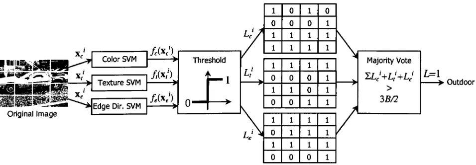
which will serve as abenchmark.

3.3.1

Majority

Classification

Assume color, texture, and edge direction feature vectorsxc', x/, and

xe'

are extractedfrom each

subblock i of a given image tessellation. The feature vectors are then classified _using the

corresponding

SVM,

in turn _producing the distance measures

/c(xc'), //(x/),

and fe(xe'). As

described in section

3.1.1,

these values measure the distance of a given feature vector from the

separating hyperplane the trained SVM decision

boundary

in feature space. A large positive

value indicates the feature vector has strong outdoor scene cues.

Conversely,

a large negative

valueindicates thefeaturevectorhas strong indoor scene cues.

Thus,

hard indoor/outdoor labels

Lc',

L,',

and Le'

can be obtained for each subblock i using a hard limiter i.e.

thresholding

the

distance measuresatzero:

4=

r

fA<)>0

co)

[0,

otherwise

I}-{1 /'(X;)>

(51)

[0,

otherwise

V,-\l- f->

A label equal to one

indicates

the subblock represents an outdoor scene. After computing the

above_equations, each subblockhas three

indoor/outdoor

labels,

one foreach feature type. Let S

representthesummation of

labels

Lj, L/,

_and

Lj

_{over all subblocks:}

S =

4+4+4

(53)

/=i

Where,

B isthe total number of subblocks (e.g. 5=4fora2x 2tessellation). An indoor/outdoor

labelcanthusbeobtainedforthewholeimage accordingto:

L=

[1,

S>3B/2

0,

otherwise

(54)

If,

forexample, color, texture, and edgedirection features are usedin a4 x4 image tessellation,

there will be 35 subblock labels. The label L=l

(outdoor)

is assigned if the subblock label

summation S is greater than halfthenumber oftotal subblocks; in thiscase 35/2=24.

However,

not all low-levelfeaturesneedbeused. For

instance,

_onlytwoofthelow-level features mightbe

extracted and classified. In this case,

25/2=16,

and _therefore, the label L=l

(outdoor)

would be

assigned if 5>16. The majorityclassifier is shown _{graphically for} a 4 x4 tessellation in Figure

10.

1 0 1 0

0 0 0

1 1 1

\

fc(*J) 1 1 1

V

Xc

ColorSVM Threshold

\

_MajorityVote

ZLj+LJ+Lj

>

3B/2

1 1 1

/,(*/) 0 0 0

Texture SVM

"^^lasffl*^

\

1 1 0

/

Original Image

fe(Xe')

Edge Dir. SVM > o

f

? 0 0 1

1 1 1

/

o 1 1

/

1 1 1

0 0 0

L=\

[image:34.613.85.563.518.684.2]

Outdoor

3.3.2

Synthesis

of

Subblock SVM Distances

This approach is _very similar to _majority classification except that the SVM distance measure is

exploited. In the_majorityclassification_approach, hard indoor/outdoorlabels

Lj, L/,

and

Lj

were

obtained

by

thresholding

/c(Xc'),

/,(x/),

and/e(xe').

Doing

_so,

however,

is equivalent _{to quantizing}

thedistancemeasures, thus

incurring

alossofinformationandprecision. Given that/c(xc'),/,(x/),

andfe(xe') aredistance measures _{corresponding} toall subblocks,

they

can be summed to obtain a

global distance measurefortheentireimage. Inother words, the subblockdistance measurescan

be synthesized to obtain a value that represents the indoor/outdoor belief for the full image.

Define threenewdistance measures_{corresponding}to theentire image:

dc=tfc)

<55>

;=i

*,=/,(*!)

(56)

1=1

de=f,fM)

(57)

i=i

Where,

5 again represents the total number of subblocks in the tessellation. A

binary

indoor/outdoor label can now obtained fromthe above synthesized distance measures _according

to:

l=

|1,

dc+dt+de>0

(5g)

0,

otherwise

As

before,

a label L=l corresponds to an outdoor scene.

Summing

the subblock distance

measures before binarization reduces the impact of any borderline subblocks, as opposed to

forcing

ahard label. This approach can stillbe usedevenifoneor more ofthelow-level features

is eliminated. If the edge direction features are excluded, for

instance,

the label L would be

obtained

by

thresholding the sum of

dc

and

d,

only. The subblock synthesis approach is shown

al

>Outdoor

Original Image

/f(xe') de=Zfe(xJ)

Figure 11. _{Graphic illustration}ofthesubblockSVMdistancesynthesis approach.

3.3.3

Second Stage SVM

In _preceding sections, two approaches were proposed to combine low-level features extracted

from image subblocks. In each case, the SVM subblock classification results were combined in

distinct ways in order to deduce the indoor/outdoor classification for the full image. A third

approach is to use a classifier engine to generalize the subblock classification results andinfer a

final indoor/outdoorclassificationforthefull image.

In this approach, the subblockSVM distance measures

fc(xc'),f,(x,'),

_andfe(xe') are synthesized as

in section 3.3.2 in orderto obtain distance measures

dc, dt,

and

de

_{using Eq.}

(55)

- (57). These

distance measures are then used to form a new color, texture, and edge direction feature vector

xcte.

Xc/e

-[dc-, dt, de\

(59)

A new RBF SVMis then trained_usingthe feature vector xcte. The output ofthis

SVM, fc,e(xcte),

thus represents an indoor/outdoor belief for the entire image. It can be said that the overall

process is atwo-stage approach. The firststage involvesextraction andclassification ofthe

low-levelsubblockfeaturesxj, x/,and xj. Thesecond stageinvolves _synthesizingthe subblockSVM

distance measures

/c(xc'),/,(x/),

and

fe(xj)

in ordertoobtainthefull imagecolor, texture,and edge [image:36.613.84.541.91.207.2]

stage SVM in order to obtain the final indoor/outdoor classification. The two-stage SVM

approachis shown_{graphically for}a4x4tessellationin Figure 12.

Original Image

d^ZfcxJ) SECONDSTAGE

4=2/,(x/) /(xJ Final

> Indoor/Outdoor Classification

[image:37.613.72.544.161.272.2]

de=Xfe(xJ)

4.

SEMANTIC

FEATURE EXTRACTION

Althoughclassifier engines can beused toestablish a _{relationship between image} primitivesand

semantic scene

understanding

_{(e.g. indoor vs.}

outdoor), the approach can be enriched

by

incorporating

additional

knowledge

that is pertinent to the semantic scene _{understanding} in question. In_{this case, the}semantic scene _{understanding in}question is whether or not aparticular

scene is indoor vs. outdoor. _{Additional knowledge thatis} pertinent tothis taskmightbe whether or notthe scene contains grass and/or _{sky regions,} for example. Ifthe scene does contain grass and/or _{sky, then} it canbe assertedthatit is an outdoor scene. Thisassertion isnot categorical, as thereare ambiguous cases such as photographstaken throughwindows.

However,

thesecases are infrequent and _generally without resolution

involving

philosophical discourse.

Hence,

it is

reasonable to assume that additional knowledge ofthe scene might reinforce the indoor/outdoor

categorization obtained _using low-level image analysis. Two inevitable questions arise. Can

additional knowledge ofthe scene be obtained reliably? And if so, how can this knowledge be

incorporated withtheaforementionedlow-level features?

Fortheapplication considered

here,

semantic scene content such as _grass,sky,

buildings,

cars and

people can be said to represent mid-level scene information in that it is less general than the

indoor vs. outdoor labeling. Prior image _{understanding} research has shown that such mid-level

scene content can be detected reliably. Some examples include vegetation detection

[51],

_sky

detection

[51,52],

and peopledetection [53].

Furthermore,

models forprobabilisticintegration of sceneinformationalsoexist.

Specifically,

the use ofBayesiannetworks for feature integration is

discussed insection 5.

Not all mid-level scene information is useful in

determining

whether or not a given image is an indoorscene or anoutdoor scene. Forexample, peoplecan bepresent in both indoorand outdoor

scenes.

However,

_only on rare occasions can grass be found indoors (e.g. a domed stadium).

Similarly,

sky regions are almost always present in outdoor scenes. Given this reasoning, the

To propose a scheme for the

detection

of grass and _sky in images is beyond the scope ofthis

work.

Instead,

reliable grass and _sky ground truth associated with animage databaseprovided

by

Kodak (see section

6.1)

was used. _{The sky} ground truth is further qualified as blue sky, cloud,

mixed _{sky, twilight, or other sky. The use of ground truth provides an upper bound on the}

indoor/outdoor

classification accuracy. To ascertain how accurate the indoor/outdoor

classification might be with computed mid-level

information,

grass and _{sky detection} schemes

developed

by

Kodakwere used. Kodak's_skydetection algorithmis asdescribed in [52]. Though

undocumented, the grass detection algorithm employs color and texture information to detect

[image:39.614.91.531.296.441.2]

grass regions. Anexampleimage andits associated grassground truthare shownin Figure 13.

5. FEATURE INTEGRATION

In _{this section, the} process of

integrating

low-level features (as thosedescribed in section

2)

and

semantic

features

(as those

described

in section

4)

for enhanced indoor/outdoor classification is discussed. An introduction to Bayesian networks probabilistic inference engines is first

provided.

5.1

Bayesian

Networks

Bayesian networks, also known as belief _networks, or _{simply Bayes nets,} provide a powerful

framework for the description of complicated probabilistic systems through simple conditional

relationships [54].

They

have become an important tool in the field of artificial

intelligence,

which is ruled

by

uncertainty.

Bayes'

theorem is one of the celebrated results of _probability

theory. It states that the posterior (or a _{posteriori) probability is described}

by

the joint

probability, which in turn, is described

by

theconditional _probability and the prior (ora_priori) probability:

Pvni!i.*5i*>.2\Em

(60)

1

P(E)

P{E)

The latterpart ofEq.

(60)

is the well-knowninversion formula. In words,it states thatthebelief

hypothesis H is true, based on new evidence E (posterior probability), can be expressed

by

the

product oftheprevious belief H is true (priorprobability) with thelikelihood thatEwill occurif Histrue(conditionalprobability).

The importance of this result is that P(H

\

E),

a

typically

difficult quantity to assess, can be

obtainedfromquantities thatare not_only moreaccessible, but usually availablefromexperiential knowledge.

Yet,

often theevidenceE isnotasingle variablebutrather,a set ofvariables. As the

numberofevidence variables

increases,

computation ofthejoint probabilitybecomesintractable.

Furthermore,

it has been observed that a _purely mathematical description of probabilistic

reasoning. Perhaps the most

striking limitation

_{of numerical approaches to}

probability is the

assessment of

independence.

Using

the previous _example, ifthe hypothesis His independent of

theevidence

E,

_then,

P(H, E)

=

P(H) P(E)

(61)

And thus, theposterior_{probabilityis} equalto theprior_probability,

P(H\E)

=

P(H,E)

=P(H)

(62)

P(E)

Inpractice, independence is gauged

by

_computing theproduct

P(H)P(E)

and

determining

whether

or not it is equal to the joint probability. Although more

formal,

it is impractical and again

deviates from human intuition. In

fact,

humans are _quickly and _confidently able to determine

independence without _computing