Unified finite element methodology for gradient elasticity

This is a repository copy of Unified finite element methodology for gradient elasticity. White Rose Research Online URL for this paper:

http://eprints.whiterose.ac.uk/90078/ Version: Accepted Version

Article:

Bagni, C. and Askes, H. (2015) Unified finite element methodology for gradient elasticity. Computers and Structures, 160. 100 - 110. ISSN 0045-7949

https://doi.org/10.1016/j.compstruc.2015.08.008

Reuse

Unless indicated otherwise, fulltext items are protected by copyright with all rights reserved. The copyright exception in section 29 of the Copyright, Designs and Patents Act 1988 allows the making of a single copy solely for the purpose of non-commercial research or private study within the limits of fair dealing. The publisher or other rights-holder may allow further reproduction and re-use of this version - refer to the White Rose Research Online record for this item. Where records identify the publisher as the copyright holder, users can verify any specific terms of use on the publisher’s website.

Takedown

If you consider content in White Rose Research Online to be in breach of UK law, please notify us by

Unified finite element methodology for gradient

elasticity

Cristian Bagnia,∗_{, Harm Askes}a

a

University of Sheffield, Department of Civil and Structural Engineering, Mappin Street, Sheffield S1 3JD, United Kingdom

Abstract

In this paper a unified finite element methodology based on gradient-elasticity

is proposed for both two- and three-dimensional problems, along with some

considerations about the best integration rules to be used and a

comprehen-sive convergence study. From the convergence study it has emerged that for

both two and three-dimensional problems, the implemented elements show

a convergence rate virtually equal to the corresponding theoretical values.

Recommendations on optimal element size are also provided. Furthermore,

the ability of the proposed methodology to remove singularities in statics

has been demonstrated through a couple of examples, in both two and three

dimensions.

Keywords: Finite element methodology; Gradient elasticity; Internal length scale; Fracture mechanics; Removal of singularity; 2D and 3D Finite

elements

∗_{Corresponding author. Tel.:+44(0)114 2227728; fax:+44(0)114 2227890}

Email addresses: [email protected](Cristian Bagni),

1. Introduction

Classical continuum theories are used to solve various fundamental

en-gineering problems and applications. Even if these theories are capable of

solving problems in which the scale of the unknowns is appreciable by the

human eye, they have been used to characterise phenomena at a very small

(atomistic) as well as extremely big (astronomic) scale. Furthermore,

classi-cal elasticity has also been recently applied to describe deformation problems

at the micron and nano-scale.

Experimental observations have suggested that, at these two last scales

of observation, classical continuum theories fail in the accurate description

of deformation phenomena. In particular, classical theories produce

singu-larities in the strain and stress fields, for example in correspondence of crack

tips and dislocation lines. Furthermore, they are not able to capture size

effects, even if the influence of size effects increases with the decrease of the

component size.

The failure of classical continuum theories in the description of the above

problems is linked to the absence of an internal length in the constitutive

equations, representative of the underlying microstructure. To overcome the

previously described deficiencies, it has been proposed to enrich the

constitu-tive equations, through the introduction of high-order gradients of particular

state variable (e.g. strains or stresses), accompanied by internal length

pa-rameters (see [1] for an overview).

The idea of using gradient elasticity to describe the mechanical behaviour

of materials and structures dates back to the second half of the 19th _century;

years (a comprehensive overview of the history of gradient elasticity can be

found in [1]).

Despite its ability to overcome the deficiencies of classical elasticity in

the solution of different problems, gradient elasticity has not found a

sig-nificant diffusion in practical applications yet. One of the principal reasons

is its non-trivial finite element implementation, mainly related to the

con-tinuity requirements imposed on the discretisation. In fact, while the

stan-dard equations of solid mechanics are usually second order partial differential

equations (p.d.e.), the governing equations of gradient elasticity are typically

fourth-order p.d.e.; this means that the discretisation of the gradient

elas-ticity equations requires at least C1_{-continuous shape functions, instead of}

the usual C0_{-continuous shape functions, which cannot be straightforwardly}

defined and implemented in a finite element methodology.

There are two main approaches followed to implement gradient elasticity

into a finite element methodology (for a more detailed overview see [1, 2]).

The first one comprehends approaches that leave the continuum mechanics

equations intact, by using Meshless methods [3–11], Penalty methods [12–

14], Hermitian finite elements [15–18], next nearest neighbour interaction

(instead of the simpler nearest neighbour interaction used in the standard

finite element software) [19], etc. The second one includes approaches that

transform the governing equations, in order to obtain less demanding

conti-nuity requirements; among these is the Ru-Aifantis theorem [20] which splits

the original fourth-order p.d.e. in two uncoupled sets of second-order p.d.e.

In this paper, we build on the finite element technology developed by [2,

point to develop a straightforward C0_{-continuous implementation. The work}

of these earlier papers is extended from 2D to 3D and higher-order elements,

whilst also a comprehensive study of optimal numerical integration rules is

provided and in-depth convergence studies have been carried out. Thus,

rec-ommendations on element types and sizes can now be made.

While in Section 2 the Ru-Aifants theory, implemented in the proposed

methodology, is briefly reviewed, in Section 3 an effective C0 _{finite element}

implementation of this theory is described. Section 4 provides details about

the best integration rules to use for each of the different implemented

fi-nite elements, whilst in Section 5 the convergence behaviours of the different

implemented elements are compared and analysed for problems without

sin-gularities and in Section 6 the same has been done for a problem characterised

by the presence of a singularity. Recommendations on optimal element size

are also provided. In Section 7 original results, obtained by applying the

proposed methodology to two different problems, are presented in order to

demonstrate the ability of the methodology to remove singularities from the

stress field for both two- and three-dimensional problems.

2. Ru-Aifantis theory of gradient elasticity

At the beginning of the 1990s, Aifantis and coworkers proposed to enrich

the constitutive relations of classical elasticity by means of the Laplacian of

the strain as [20, 22, 23]

σij =Cijkl(εkl−ℓ2εkl,mm) (1)

where σij and εkl are, respectively, the stress and strain tensor, Cijkl is the

equations are

Cijkl(uk,jl−ℓ2uk,jlmm) +bi = 0 (2)

where uk is the displacement field and bi are the body forces.

In a later work [20], Ru and Aifantis proposed an operator split, which allows the solution of the fourth-order equilibrium Eq. (2) as a decoupled

sequence of two sets of second-order p.d.e., that is

Cijkluck,jl+bi = 0 (3)

followed by the following reaction-diffusion equation

ug_k−ℓ2ug_k,mm =uc_k (4)

that represents the relation between the local displacements uc

i, obtained by

solving the equations of classical elasticity Eq. (3) (carrying for this reason

the superscript c), and the non-local displacementsug_i, affected by the

gradi-ent activity (superscript g), which are the same displacements appearing in

Eq. (2).

Substituting Eq. (4) into Eq. (3), the original Eq. (2) are recovered and

imposing suitable boundary conditions the solution of Eqs. (3) and (4)

co-incides with that of the original Eq. (2). Nevertheless, the most interesting

aspect of Eqs. (3) and (4) is their uncoupled format, which significantly

sim-plifies both the analytical and numerical solution of the system of equations.

The first Ru-Aifantis approach introduces the gradient-enrichment in

terms of displacements, as given in Eq. (4), but through a simple

differ-entiation it is also possible to express the gradient-enrichment in terms of

strains [2, 24, 25], that is

εg_kl−ℓ2εg_kl,mm=εc_kl = 1 2(u

c

or stresses as [2, 26]

σ_ijg −ℓ2σg_ij,mm =Cijkluck,l (6)

3. Finite element implementation

As briefly explained in Section 2 and in more details in [1], the Ru-Aifantis

theorem consists in solving two uncoupled sets of second-order p.d.e. instead

of the original fourth-order p.d.e., which significantly simplifies the solution

of the problem. From now on matrix-vector notation is adopted, instead of

the index notation used in Section 2.

The first step of the Ru-Aifantis theory consists in determining the local

displacements uc by solving the second-order p.d.e. of classical elasticity:

LTCLuc+b= 0 (7)

wherebare the body forces,Cis the constitutive matrix, while the derivative

operator L is defined as

L =       ∂

∂x 0 0

∂ ∂y ∂ ∂z 0 0 ∂ ∂y 0 ∂ ∂x 0 ∂ ∂z

0 0 ∂

∂z 0 ∂ ∂x ∂ ∂y       T (8)

The continuum local displacements uc =

uc

x, ucy, ucz

T

are expressed in

terms of the nodal local displacements dc =

dc

1x, dc1y, dc1z, dc2x, dc2y, dc2z, . . .

T

traditional shape functions Ni and can be written as:

Nu =



   

N1 0 0 N2 0 0 . . .

0 N1 0 0 N2 0 . . .

0 0 N1 0 0 N2 . . .

     (9)

Considering the finite element discretisation just described and

integrat-ing by parts, the weak form of Eq. (7) reads

Z

Ω

BT_uCBudΩdc ≡Kdc =f (10)

whereKis the stiffness matrix,Bu =LNu is the strain-displacement matrix

andf is the force vector, where the contributions of both the body forces and

the external tractions are included.

At this point, knowing the local displacementsuc from the previous step,

it is possible to evaluate the stress field by solving the second set of equations

(second step):

(σg −ℓ2∇2σg) = CLuc (11)

where σg is the non-local stress tensor and the derivative operator ∇ is

defined as ∇=       ∂ ∂x ∂ ∂y ∂ ∂z      

with ∇2 _{≡ ∇}T_{∇ (12)}

Considering the weak form of Eq. (11) and integrating by parts, we obtain

Z

Ω

wTσg+ℓ2

∂wT

∂x ∂σg

∂x + ∂wT

∂y ∂σg

∂y + ∂wT

∂z ∂σg

∂z

dΩ −

−

I

Γ

wTℓ2(n· ∇σg)dΓ = Z

Ω

wheren = [nx ny nz]T contains the components of the normal vector to the

boundary Γ and w is the test function vector.

Since the same finite element mesh can be used for both the first step,

described above, and this second step, the same shape functions, previously

used to discretise the displacements, can be used also for the discretisation

of the stresses, making the solution of the problem much easier. Hence, the

vector of the continuum non-local stresses σg is related to the vector of the

nodal non-local stresses sg through the relation σg =N_σsg, where N_σ is an

expanded form of the shape function matrix Nu given in Eq. (9), in order to

accommodate all the non-local stress components.

Finally, using the same shape functionsNσ to discretise the test function

vector w and recalling that uc = Nudc, the resulting system of equations

reads

Z

Ω

NT_σNσ+ℓ2

∂NT_σ

∂x ∂N_σ

∂x + ∂NT_σ

∂y ∂N_σ

∂y + ∂NT_σ

∂z ∂N_σ

∂z

dΩsg =

=

Z

Ω

NT_σCBudΩdc (14)

As can be noted, in passing from Eq. (13) to Eq. (14) the boundary integral

H

Γδσ

gT_ℓ2_{(n· ∇σ}g_{)dΓ has disappeared. This is due to the fact that}

• if essential boundary conditions are used σg is known (usually the

condition σg =σc is chosen), therefore δσg = 0;

• if natural boundary conditions are used the condition n· ∇σg = 0 is

chosen.

4. Numerical integration

To solve the first and second step of the Ru-Aifantis theory described

above (i.e. Eqs. (10) and (14)) the Gauss quadrature rule has been adopted.

Since the first step of the Ru-Aifantis theory consists in the solution of

the second-order p.d.e. of classical elasticity (10), for the numerical

inte-gration of the stiffness matrix K, the usual number of integration points is

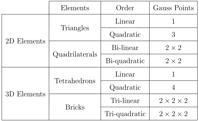
used for each kind of implemented elements, as summarised in Table 1. It

must be noted that for the bi-quadratic serendipity quadrilateral and the

tri-quadratic serendipity brick elements, an under-integration is adopted.

Table 1. Number of Gauss points used in the first step of the Ru-Aifantis theory.

Elements Order Gauss Points

2D Elements

Triangles Linear 1

Quadratic 3

Quadrilaterals Bi-linear 2×2 Bi-quadratic 2×2

3D Elements

Tetrahedrons Linear 1

Quadratic 4

Bricks Tri-linear 2×2×2 Tri-quadratic 2×2×2

At this point, the most interesting aspect to investigate is the integration

rule to use in the second step of the Ru-Aifantis theory and, in particular,

most desirable solution would be, obviously, the possibility to use the same

integration rule used in the first step of the Ru-Aifantis theory.

However, the applicability of such a solution is not obvious and would

need to be demonstrated. In fact while for the first step of the Ru-Aifantis

theory the order of the stiffness matrix (which has to be integrated) is two

times the order of the derivative of the shape functions, in the second step

the order of the integrand part (of the term in the left side of Eq. (14)) is two

times the order of the shape functions themselves; this means that for exact

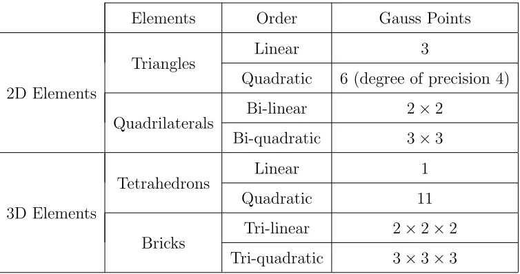
integration, higher order integration rules are needed as listed in Table 2.

Hence, in other terms, the problem is to prove if it is possible to

under-integrate (i.e. use integration rules with a lower order than that necessary

for the exact integration) the left part of Eq. (14) for both ℓ= 0 and ℓ 6= 0.

Unfortunately, this is not always possible, as described afterwards.

The investigation has been carried out through a study of the eigenvalues

of the matrix M+ℓ2_{D when ℓ 6= 0 and, obviously, of matrix M on its own}

whenℓ = 0, whereM=R

ΩN T

σNσ dΩ is the first matrix term of the left

inte-gral in Eq. (14) similar to a mass matrix, whileD =R

Ω

∂NT σ

∂x ∂Nσ

∂x + ∂NT

σ

∂y ∂Nσ

∂y + ∂NT

σ

∂z ∂Nσ

∂z

dΩ

is the second matrix term similar to a diffusivity matrix. In particular, to

avoid rank deficiencies all the eigenvalues must be non-zero, which means

that zero energy modes are not admitted.

From the performed studies it turned out that, whenℓ= 0, it is possible

to use the same integration rule only for the linear quadrilateral, tetrahedron

and brick elements, while for the other five types of elements higher order

integration rules are needed (the minimum number of integration points is

to the contribution of the matrix D, it is possible to use the same integration

rule, used in the first step, for every type of finite element.

Table 2. Number of Gauss points formally required in the second step of the Ru-Aifantis

theory.

Elements Order Gauss Points

2D Elements

Triangles Linear 3

Quadratic 6 (degree of precision 4)

Quadrilaterals Bi-linear 2×2 Bi-quadratic 3×3

3D Elements

Tetrahedrons Linear 1

Quadratic 11

Bricks Tri-linear 2×2×2 Tri-quadratic 3×3×3

4.1. Shear locking

As well known, in the case of bending-dominant problems, especially for

fully integrated linear elements, the numerical solution of the problem can

be affected by shear locking, leading to an unphysically stiffer behaviour

of the analysed component. To check the occurrence of this phenomenon,

the proposed methodology has been applied to model a classical bending

problem. The results of the aforementioned analysis have shown that the

numerical solution of the second step of the Ru-Aifantis theory (Eq. (14))

is not affected by locking effects, even in the case of fully integrated linear

elements, while the usual selective integration rules may be applied for the

5. Error estimation and convergence study

Now that the most suitable integration rules have been identified for each

kind of finite element, the attention can be focused on the error estimation

of the new methodology; in particular the convergence rate of the different

finite elements has been studied for some simple problems.

To determine the convergence rate, the L2-norm error defined as

kek2 =

kσe−σck

kσek

(15)

where σe and σc are, respectively, the exact and calculated values of the

stresses, has been plotted against the number of degrees of freedom (nDoF).

From the theory [27] it is well known that the error on displacements is

proportional to the nDoF as

eu ≃O(nDoF)− n+1

k = O(nDoF)p (16)

For what concerns the stresses, in the proposed methodology they are

calculated from Eq. (14) as primary variable, instead of secondary variable

as it happens in standard finite element methodologies, based on classical

elasticity. For this reason, the error on stresses is still proportional to the

nDoF, but with a different rate respect to classical elasticity. In particular,

for a Helmholtz equation like Eq. (14), the proportionality is given by [28]:

eσ ≃O(nDoF)− n+1

k = O(nDoF)p (17)

where n is the polynomial order and k = 2,3 for 2D and 3D problems,

respectively.

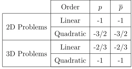
bi-logarithmic system of axes is a straight line, whose slope represents the

convergence rate p of the numerical solution to the exact solution. The

theoretical convergence rates are summarised in Table 3.

Table 3. Theoretical convergence rates in the determination of the displacements (p) and

stresses (p).

Order p p

2D Problems Linear -1 -1 Quadratic -3/2 -3/2

3D Problems Linear -2/3 -2/3 Quadratic -1 -1

5.1. Internally pressurised hollow cylinder

To test the convergence rate of the bi-dimensional elements, the problem

of a cylinder subjected to an internal pressure pi shown in Fig. 1 has been

analysed. The geometrical and material parameters of the problem are b =

4 m, a= 1 m, E = 109 _N/m2_{, ν = 0.25 and ℓ = 0.1 m. An internal pressure}

pi = 107 N/m2 is applied.

Due to the symmetry of the problem only a quarter of the vessel has been

modelled. The domain has been modelled with all four types of implemented

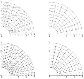
2D finite elements, starting from a coarse mesh of 8×8 elements and

per-forming then a mesh refinement by doubling the number of elements along

each side until a mesh of 256×256 elements is obtained. All the employed

meshes are shown in Fig. 2.

The boundary conditions accompanying Eq. (10) are taken as

homoge-neous essential so that the circumferential displacements uθ are null along

the two axes of symmetry, while those associated to Eq. (14) are chosen as

Fig. 2. Cylinder subject to an internal pressure: employed meshes for linear (top-left)

and quadratic (bottom-left) triangular elements, bi-linear (top-right) and bi-quadratic

(bottom-right) quadrilateral elements.

To define the error, the numerical solutions obtained using the new

method-ology have been compared with the exact solution approximated using

Fig. 3. Cylinder subject to an internal pressure: displacements error (left) and stresses

er-ror (right) versus number of Degrees of Freedom. The slope of the straight lines represents

the convergence rate of the numerical solution to the exact solution.

In Fig. 3 the convergence behaviour of all the implemented bi-dimensional

elements is shown, for both displacements and stresses. It can be seen that

the numerically obtained convergence rates are in good agreement with the

theoretical predictions given in Table 3.

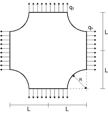
5.2. Cross-shape specimen

The second problem is the case of a cross-shape specimen subjected to

a uniform tensile state at the end of the arms as shown in Fig. 4. The

geometrical and material parameters of the problem are R = 1 m, L = 2 m,

E = 109 _N/m2_{,ν = 0.25 andℓ= 0.1 m. Distributed loads q}

x= qy = 1000 N/m

Fig. 4. Cross-shape specimen: geometry and loading conditions.

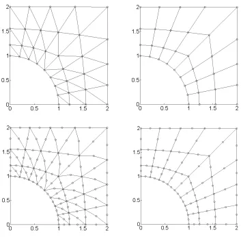
Also in this case, for symmetry reasons, only a quarter of the specimen has

been modelled using all the different types of finite elements implemented,

starting also in this case with a coarse mesh as shown in Fig. 5. Afterwords,

a mesh refinement has been performed, running four other meshes obtained

doubling the number of elements, in both radial and circumferential

direc-tions, of the previous one.

The boundary conditions accompanying Eq. (10) are taken as

homoge-neous essential so that the displacements in x-directionux and in y-direction uy are null along the vertical and horizontal axes of symmetry, respectively.

For what concerns Eq. (14), instead, the boundary conditions are chosen as

Fig. 5. Cross-shape specimen: employed meshes for linear (top-left) and quadratic

(bottom-left) triangular elements, bi-linear (top-right) and bi-quadratic (bottom-right)

quadrilateral elements.

To define the error, the numerical solutions obtained using the new

method-ology have been compared with the exact solution obtained applying the

Fig. 6. Cross-shape specimen: displacements error (left) and stresses error (right) versus

number of Degrees of Freedom. The slope of the straight lines represents the convergence

rate of the numerical solution to the exact solution.

Fig. 6 shows the convergence behaviour of all the implemented bi-dimensional

elements in the determination of both displacements and stresses; again, this

is in line with the theoretical predictions.

5.3. Internally pressurised hollow sphere

For what concerns the convergence rate of the three-dimensional elements,

the problem of a sphere subjected to an internal pressure pi shown in Fig. 7

has been studied. The geometrical and material parameters of the problem

are b = 1 m,a= 0.5 m, E = 109 _N/m2_{,ν = 0.25 and ℓ= 0.1 m. An internal}

pressure pi = 107 N/m2 is applied.

Due to the symmetry of the problem only an eighth of the sphere has been

modelled. The domain has been modelled with all four types of implemented

3D finite elements, starting from a coarse mesh, as shown in Fig. 7 for the

tri-linear brick elements, and performing then a uniform mesh refinement.

The boundary conditions related to Eq. (10) are taken ashomogeneous

of symmetry, while for what concerns Eq. (14) they are chosen as

homoge-neous natural throughout, like in the previous two examples.

Fig. 7. Hollow sphere subject to an internal pressure: geometry and loading conditions

(left), initial mesh (right).

To define the error, the numerical solutions obtained using the new

method-ology have again been compared with the exact solution obtained applying

the Richardson extrapolation.

Fig. 8. Hollow sphere subject to an internal pressure: displacements error (left) and

stresses error (right) versus number of Degrees of Freedom. The slope of the straight lines

represents the convergence rate of the numerical solution to the exact solution.

elements in the determination of both displacements and stresses. It can be

observed that, overall, the numerical solutions converge to the relative exact

solutions as theoretically expected, except for the quadratic tetrahedrons and

the tri-quadratic bricks, which appear to be slightly, but not much, slower

than theoretically predicted, in the determination of the displacements.

6. Convergence in presence of singularities and recommendations

on optimum element size

As mentioned in Section 1, one of the features of gradient elasticity is

the ability to remove singularities from the stress and strain fields as those

emerging in correspondence of crack tips. Problems characterised by the

presence of cracks represent the most demanding case from the convergence

point of view and, as a consequence of this, also in terms of element size in

the vicinity of the crack tip. Hence, the study of the convergence behaviour

of the implemented gradient-enriched finite elements in presence of cracks is

of prime importance.

To fulfil this interest, the mode I fracture problem shown in Fig. 9 and

presented in [1] has been analysed, using all the four implemented

two-dimensional elements. The geometrical and material parameters of the

prob-lem are L= 1 mm,E = 1000 N/mm2_{, ν = 0.25 and ℓ= 0.1 mm. Prescribed}

displacementsu= 0.01 mm are applied at the top and bottom edges. Due to

the symmetry only the top-right quarter has been modelled, with 4×4, 8×8,

16×16, 32×32 and 64×64 bi-linear and bi-quadratic quadrilateral elements

and with the double of linear and quadratic triangular elements (where the

two triangles).

Fig. 9. Mode I fracture problem: geometry and boundary conditions. The crack is

represented by the solid line.

Two different options are considered for the boundary conditions

accom-panying Eq. (13):

• Option 1: essential, that is the non-local stress components are

pre-scribed so that σg = σc on free boundaries. In the present example:

σg

xx = 0 on the vertical edges, σgyy = 0 on the face of the crack and

σg

xy = 0 everywhere.

• Option 2: homogeneous natural throughout, that is n· ∇σg = 0.

To determine the convergence rate, the L2-norm error defined in Section 5

has been plotted against the nDoF, as shown in Fig. 10.

From the theory [27] it is well known that, in problems with singularities,

the error on classical stresses is proportional to the nDoF as

eσ ≃O(nDoF)−[min(λ,n)]/2 = O(nDoF)p˜ (18)

where λ= 0.5 for a nearly closed crack.

system of axes is still a straight line, whose slope represents the convergence

rate ˜p of the numerical solution to the exact solution, which in this case is

˜

p= 0.25 for both linear and quadratic elements.

To define the error, the numerical solutions obtained using the new

method-ology have been compared with the exact solution approximated using

Richard-son extrapolation.

Fig. 10 shows that, in presence of singularities, both linear and quadratic

elements are characterised by approximatively the same convergence rate

(in accordance with Eq. (18)), but higher than the correspondent theoretical

value defined in Eq. (18), for what concerns the determination of the stresses.

This higher convergence rate is due to two main causes:

• removal of singularities from the numerical solution;

• gradient-enriched stresses calculated as primary variables, instead of

secondary variables (as for classical stresses).

Furthermore, it can be observed that, while the application of the second

option of the boundary conditions leads to a uniform convergence rate equal

to about 0.8, adopting the first option all the elements are characterised by

an initial convergence rate of about 0.3, reaching the same convergence rate

Fig. 10. Mode I fracture problem: stresses error versus number of Degrees of Freedom

for the first (left) and the second (right) option of boundary conditions. The slope of

the straight lines represents the convergence rate of the numerical solution to the exact

solution.

Since, as mentioned before, the case of a sharp crack represents the most

demanding problem in terms of convergence, it is now possible to provide

recommendations on optimal element size. In particular, in Table 4 the ratio

between the element size and the length scale ℓ, necessary to guarantee an

error of about 5% or lower, is summarised for the different elements.

The recommendations provided in Table 4 have a very important

mean-ing from the commercial point of view, because they show that, applymean-ing

the proposed methodology, a relatively coarse mesh is enough to obtain a

solution affected by an acceptable error, with evident benefits in terms of

Table 4. Recommended optimal element size, to guarantee an error of 5% or lower.

Boundary Conditions Elements Order Element size/ℓ

Option 1

(essential b.c.)

Triangles Linear 1/3

Quadratic 1/4

Quadrilaterals Bi-linear 1/3 Bi-quadratic 1/3

Option 2

(natural b.c.)

Triangles Linear 1

Quadratic 5/2

Quadrilaterals Bi-linear 3/2 Bi-quadratic 5/2

7. Applications

Once the new methodology was fully implemented, it has been applied

to a two- and three-dimensional problem, in order to show the ability of the

methodology in removing singularities.

7.1. Mode I fracture

The mode I fracture problem described in Section 6 has been analysed,

using all the four implemented two-dimensional elements, in order to check

the quality of the results.

In Fig. 11 σxx and σyy profiles along the x-axis, obtained applying both

the options on the boundary conditions, are plotted and compared; it can

be seen that the application of the different boundary conditions produces

Fig. 11. Mode I fracture problem: comparison of theσxx(left) andσyy (right) values for

y = 0, obtained employing the different kind of finite elements and both the options for

the boundary conditions.

Fig. 12. Mode I fracture problem: surface plots of stress component σxx with

homo-geneous essential boundary conditions. Comparison between the results obtained in [1]

using bi-linear quadrilateral elements (left) and those obtained employing the implemented

linear triangular elements (right).

The stress fields obtained using the 32×32 mesh, with all the four types

of elements, have been compared with the stress fields presented in [1] using

32×32 bi-linear quadrilateral elements and, as shown in Fig. 12, the

(in Fig. 12 only the σxx field, obtained using the linear triangular elements

and the second option for the boundary conditions, is compared with the

corresponding one presented in [1]).

But the most significant aspect is that, introducing a gradient

enrich-ment, the singularities in the stress field are removed; in fact, as shown in

Fig. 13, applying classical elasticity the solution does not converge to a finite

value upon mesh refinement and an unbounded peak is detected in

corre-spondence of the crack tip, while introducing a gradient enrichment in the

governing equations, refining the mesh the solution is not anymore singular

and converges towards a unique finite value.

Fig. 13. Mode I fracture problem: σyy profiles along x-axis obtained by applying

clas-sical elasticity (left) and gradient elasticity (right) and the first option on the boundary

conditions, upon mesh refinement.

7.2. Beams-column joint

In order to show the ability of the proposed methodology to remove the

singularities also in three-dimensional problems, the problem shown in Fig. 14

are L = 2.4 m, a = 0.4 m, E = 1000 N/mm2_{, ν = 0.25 and ℓ = 0.03 m.}

Prescribed surface distributed loads q = 105 _N/m2 _{are applied at the free}

end of the two beams, while the column is fully restrained at its base. The

boundary conditions associated to Eq. (14) are chosen as homogeneous nat-ural throughout, that is n· ∇σg = 0. The domain has been modelled using

128 (Fig. 14), 1024, 8192 and 65536 linear brick elements.

Fig. 14. Beams-column joint: geometry and loading conditions (left), starting mesh

(right).

In Fig. 15 the normal stress σxx and the shear stress σxy obtained by

applying both classical elasticity (ℓ = 0.00m) and gradient elasticity (ℓ =

0.03m) are plotted along a vertical edge of the column (x = 0.4, y = 0.4,

0.0 ≤ z ≤ 2.4), while in Fig. 16 the normal stress σxx is plotted along the

Fig. 15. Beams-column joint: profiles ofσxx (top row) and σxy (bottom row), along a

column vertical edge (x= 0.4,y= 0.4, 0.0≤z≤2.4), for both classical (left column) and

gradient (right column) elasticity, over mesh refinement.

Fig. 16. Beams-column joint: profiles of σxx, along the beam in y-direction (x= 0.2,

0.0 ≤ y ≤ 2.4, z = 2.0), for both classical (left column) and gradient (right column)

Both figures clearly show the ability of the proposed methodology to

re-move singularities from the stress fields; in fact while the use of classical

elasticity leads to singular solutions in correspondence of the stress

concen-trators, if a gradient enrichment is introduced in the governing equations of

the problem, the solutions are not singular anymore, converging to a unique

finite solution. Hence the ability of the proposed methodology to remove the

singularities is confirmed also for three dimensional problems.

8. Conclusions

In this paper a unified FE methodology based on gradient-elasticity, for

both two- and three-dimensional finite elements, has been presented,

includ-ing Gauss integration rules and error estimation.

The proposed methodology has been applied to both two- and

three-dimensional simple problems without singularities and it has been found

that, overall, the numerically obtained convergence rates are well in line

with theoretical predictions.

The convergence rate of the proposed methodology has been also

anal-ysed in presence of singularities, showing that both linear and quadratic

elements are characterised by a convergence rate higher than the

theoreti-cal value typitheoreti-cal of finite element methodologies based on classitheoreti-cal elasticity.

This is mainly due to the ability of gradient elasticity to remove singularities

from the numerical solution and to the fact that, in the proposed

method-ology, the gradient-enriched stresses are determined as primary variables,

instead of secondary variables as for classical elasticity-based finite element

been provided, highlighting the ability of the proposed methodology to

pro-duce solutions affected by acceptable errors using relatively coarse meshes,

with consequent advantages in terms of computational cost.

Furthermore, the proposed methodology has been applied to a couple of

problems that classical elasticity fails to describe accurately, in particular

to a two-dimensional mode I fracture problem, through which it has been

shown that the different implemented finite elements produce comparable

results (as expected) and that the application of different boundary

condi-tions leads to limited and acceptable differences in the final solution; and

to a three-dimensional problem characterised by stress concentrators. These

two examples highlight the ability of the proposed methodology to remove

the singularities from the stress fields, for both two- and three-dimensional

problems.

Acknowledgements

The authors gratefully acknowledge financial support from Safe

Technol-ogy Ltd.

References

[1] H. Askes and E. C. Aifantis. Gradient elasticity in statics and

dy-namics: An overview of formulations, length scale identification

pro-cedures, finite element implementations and new results. Interna-tional Journal of Solids and Structures, 48(13):1962–1990, 2011. doi:

[2] H. Askes, I. Morata, and E. C. Aifantis. Finite element analysis with

staggered gradient elasticity. Computers & Structures, 86:1266–1279, 2008. doi: 10.1016/j.compstruc.2007.11.002.

[3] H. Askes, J. Pamin, and R. de Borst. Dispersion analysis and

element-free Galerkin solutions of second- and fourth-order gradient-enhanced

damage models. International Journal for Numerical Methods in

Engi-neering, 49:811–832, 2000.

[4] H. Askes and E. C. Aifantis. Numerical modelling of size effects with

gradient elasticity - formulation, meshless discretization and examples.

International Journal of Fracture, 117:347–358, 2002.

[5] H. Askes and L. J. Sluys. Explicit and implicit gradient series in

dam-age mechanics. European Journal of Mechanics - A/Solids, 21:379–390,

2002.

[6] H. Askes, A.S.J. Suiker, and L. J. Sluys. A classification of higher-order

strain-gradient models - linear analysis. Archive of Applied Mechanics,

72:171–188, 2002.

[7] H. Askes and L. J. Sluys. A classification of higher-order strain-gradient

models in damage mechanics. Archive of Applied Mechanics, 73:448–465, 2003.

[8] J. Pamin, H. Askes, and R. de Borst. Two gradient plasticity theories

discretized with the element-free Galerkin method. Computer Meth-ods in Applied Mechanics and Engineering, 192:2377–2403, 2003. doi:

[9] Z. Tang, S. Shen, and S.N. Atluri. Analysis of materials with

strain-gradient effects: a meshless local Petrov-Galerkin (MLPG) approach,

with nodal displacements only. Computer Modeling in Engineering &

Sciences, 4:177–196, 2003.

[10] I. Tsagrakis and E. C. Aifantis. Element-free Galerkin implementation

of gradient plasticity. Part I: formulation and application to 1D strain

localization. Journal of the Mechanical Behavior of Materials, 14:199–

231, 2003.

[11] I. Tsagrakis and E. C. Aifantis. Element-free Galerkin implementation

of gradient plasticity. Part II: applications to 2D strain localization and

size effects. Journal of the Mechanical Behavior of Materials, 14:233–

253, 2003.

[12] J. Pamin. Gradient-dependent plasticity in numerical simulation of

local-ization phenomena. Dissertation, Delft University of Technology, 1994.

[13] A. Zervos. Finite elements for elasticity with microstructure and

gra-dient elasticity. International Journal for Numerical Methods in Engi-neering, 73(4):564–595, 2008. doi: 10.1002/nme.2093.

[14] A. Zervos, S. Papanicolopulos, and I. Vardoulakis. Two finite-element

discretizations for gradient elasticity. Journal of Engineering Me-chanics ASCE, 135(3):203–213, 2009. doi:

10.1061/(ASCE)0733-9399(2009)135:3(203).

Inter-national Journal for Numerical Methods in Engineering, 37:3489–3519,

1994.

[16] A. Zervos, P. Papanastasiou, and I. Vardoulakis. A finite elements

dis-placement formulation for gradient elastoplasticity. International Jour-nal for Numerical Methods in Engineering, 50:1369–1388, 2001.

[17] A. Zervos, P. Papanastasiou, and I. Vardoulakis. Modelling of

local-isation and scale effect in thick-walled cylinders with gradient

elasto-plasticity. International Journal of Solids and Structures, 38:5081–5095, 2001.

[18] S. A. Papanicolopulos, A. Zervos, and I. Vardoulakis. A

three-dimensionalC1 _{finite element for gradient elasticity.International}

Jour-nal for Numerical Methods in Engineering, 77:1396–1415, 2009. doi: 10.1002/nme.2449.

[19] F. Cirak, M. Ortiz, and P. Schr¨oder. Subdivision surface: a new

paradigm for thin-shell finite-element analysis. International Journal

for Numerical Methods in Engineering, 47:2039–2072, 2000.

[20] C. Q. Ru and E. C. Aifantis. A simple approach to solve boundary-value

problems in gradient elasticity. Acta Mechanica, 101:59–68, 1993. doi:

10.1007/BF01175597.

[21] L. Tenek and E. C. Aifantis. A two-dimensional finite element

[22] E. C. Aifantis. On the role of gradients in the localization of deformation

and fracture.International Journal of Engineering Science, 30(10):1279– 1299, 1992. doi: 10.1016/0020-7225(92)90141-3.

[23] S.B. Altan and E. C. Aifantis. On the structure of the mode III

crack-tip in gradient elasticity. Scripta Metallurgica et Materialia, 26:319–324,

1992.

[24] M. Gutkin and E. C. Aifantis. Edge dislocation in gradient elasticity.

Scripta Materialia, 36:129–135, 1997.

[25] M. Gutkin and E. C. Aifantis. Dislocations in the theory of gradient

elasticity. Scripta Materialia, 40:559–566, 1999.

[26] M. Gutkin. Nanoscopics of dislocations and disclinations in gradient

elasticity. Reviews on Advanced Materials Science, 1:27–60, 2000.

[27] O.C. Zienkiewicz and R.L. Taylor. The Finite Element Method, volume 1 – The Basis. Butterworth-Heinemann, 5th _{edition, 2000. ISBN 0 7506}

5049 4.

[28] F. Ihlenburg and I. Babuˇska. Finite Element Solution of the Helmholtz

Equation with High Wave Number Part I: The h-Version of the FEM.

Computers & Mathematics with Applications, 30(9):9–37, 1995.

[29] L. F. Richardson. The approximate arithmetical solution by finite

dif-ferences of physical problems involving differential equations, with an

En-gineering Sciences, 210(459-470):307–357, 1911. ISSN 0264-3952. doi: