arbitrary degree: linear dependencies, partition of unity property, nesting behaviour and
local refinement
.
White Rose Research Online URL for this paper:
http://eprints.whiterose.ac.uk/100671/
Version: Accepted Version
Article:
May, S., Vignollet, J. and de Borst, R. orcid.org/0000-0002-3457-3574 (2015) The role of
the Bézier extraction operator for T-splines of arbitrary degree: linear dependencies,
partition of unity property, nesting behaviour and local refinement. International Journal for
Numerical Methods in Engineering, 103 (8). pp. 547-581. ISSN 0029-5981
https://doi.org/10.1002/nme.4902
[email protected] https://eprints.whiterose.ac.uk/ Reuse
Unless indicated otherwise, fulltext items are protected by copyright with all rights reserved. The copyright exception in section 29 of the Copyright, Designs and Patents Act 1988 allows the making of a single copy solely for the purpose of non-commercial research or private study within the limits of fair dealing. The publisher or other rights-holder may allow further reproduction and re-use of this version - refer to the White Rose Research Online record for this item. Where records identify the publisher as the copyright holder, users can verify any specific terms of use on the publisher’s website.
Takedown
If you consider content in White Rose Research Online to be in breach of UK law, please notify us by
Published online in Wiley InterScience (www.interscience.wiley.com). DOI: 10.1002/nme
The role of the B´ezier extraction operator for T-splines of arbitrary
degree: linear dependencies, partition of unity property, nesting
behaviour, and local refinement
Stefan May
1∗, Julien Vignollet
1, Ren´e de Borst
11University of Glasgow, School of Engineering, Rankine Building, Oakfield Avenue, Glasgow G12 8LT, UK.
SUMMARY
We determine linear dependencies and the partition of unity property of T-spline meshes of arbitrary degree using the B´ezier extraction operator. Local refinement strategies for standard, semi-standard and non-standard T-splines – also by making use of the B´ezier extraction operator – are presented for meshes of even and odd polynomial degree. A technique is presented to determine the nesting between two T-spline meshes, again exploiting the B´ezier extraction operator. Finally, the hierarchical refinement of standard, semi-standard and non-standard T-spline meshes is discussed. This technique utilises the reconstruction operator, which is the inverse of the B´ezier extraction operator. Copyright c0000 John Wiley & Sons, Ltd.
Received . . .
KEY WORDS: T-splines, isogeometric analysis, B´ezier extraction, linear dependency, partition of unity, hierarchical refinement
1. INTRODUCTION
Isogeometric analysis was introduced in [1]. It is based on the concept that the same shape functions are used to represent the geometry and to approximate the field variables. Initially, Non-Uniform Rational B-Splines (NURBS) have been used as shape functions in isogeometric analysis. Since NURBS have a tensor product structure, refinement occurs globally. Furthermore, it can be difficult to model watertight surfaces with NURBS patches. T-splines, which can be conceived as a generalisation of NURBS, were introduced in [2, 3] and do not suffer from the limitations that are inherent in NURBS. Local refinement is now possible and watertight surfaces can be created. Moreover, T-splines allow for the reduction of superfluous control points. Use of T-spline blending functions as shape functions in a finite element context was proposed in [4, 5].
NURBS and T-splines meet a growing acceptance in the engineering community, which is considerably facilitated by the technique of B´ezier extraction [6, 7]. B´ezier extraction allows for an implementation that is identical to that typically used in finite element codes. However, in [8] the concern was raised that for T-spline meshes, linear independence – which is a necessary condition to perform the analysis – is not an inherent property of the blending functions. In [9], a definition for analysis-suitable T-spline meshes was proposed which results in a mildly restricted subset of T-splines. A topological algorithm was developed as well: a T-spline mesh was deemed analysis-suitable when there are no two orthogonal T-node extensions which intersect in the extended T-spline mesh. A considerable amount of research has been spent since then on the
∗Correspondence to: Stefan May, University of Glasgow, School of Engineering, Oakfield Avenue, Rankine Building,
properties of analysis-suitable T-spline meshes [10–12]. In [13] an algorithm based on the T-spline mesh topology was presented to refine analysis-suitable T-spline meshes. Recently, a hierarchical refinement algorithm for analysis-suitable T-splines based on the reconstruction operator was introduced in [14, 15]. Furthermore, the partition of unity property and linear dependencies for T-splines without multiple knots were investigated in [16] and [17], respectively.
Using the B´ezier extraction procedure [7], each blending function can be defined in a normalised fashion by a linear combination of Bernstein polynomials. We will show that linear dependencies and the partition of unity property can be determined for T-spline meshes with the B´ezier extraction operator at hand. It will be demonstrated that this approach can be applied to T-spline meshes of arbitrary degree. The B´ezier extraction operator also enables to determine the nesting behaviour between two T-spline meshes. Moreover, we show how standard, semi-standard and non-standard T-spline meshes can be refined locally using information from the B´ezier extraction operator.
This paper is organised as follows. In the first section we give a concise description of T-splines. Next, we present a brief overview on the construction of the B´ezier extraction operator for T-splines. Subsequently, linear dependence and the partition of unity property of T-spline meshes are investigated using the B´ezier extraction operator. In Section 5 a refinement method is proposed for T-spline meshes by adding anchors while the B´ezier extraction operator is utilised for the determination of the nesting behaviour between two T-spline meshes. The capabilities of the method are demonstrated for meshes of even and of odd polynomial degree. Finally, a technique is introduced to refine hierarchically standard, semi-standard and non-standard T-spline meshes.
2. T-SPLINES
This section provides a brief overview of T-splines. For a more elaborate demonstration of T-splines in a finite element environment we refer to [5]. Note, that herein we limit ourselves to two-dimensional problems but the methods developed in this paper can also be used in three dimensions – the only requirement is that we are able to elaborate the B´ezier extraction operator. Index notation is adopted throughout with respect to a Cartesian frame.
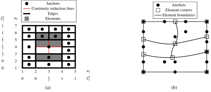
2.1. Definition of the domains
In Figure 1 the physical domain (xℓ), the parent domain (ξ˜ℓ), the index domain (uℓ), the parameter domain (ξu
ℓ), and the sub-parameter domain (ξℓ) are shown for T-splines. Each element e can be mapped from the physical domain xℓ onto the parent domain ξ˜ℓ∈[−1,1], where Gaussian integration can be carried out. The sub-parameter domain ξℓ is obtained when only the unique values of the parameter domainξu
ℓ are considered.
2.2. Definition of the local knot vector
The index domain in Figure 1 represents a tiling of a region inR2while all edges of each rectangle have a positive integer value. T-spline meshes of odd and of even polynomial order have to be treated differently when defining the local knot vectors from the parameter domain. The local knot vectors are necessary to define the blending functions, see Section 2.3.
For a T-spline mesh of even degree pℓ in both directions, a so-called anchor – to which a single multivariate blending function is attached – is placed in the centre of each rectangle, see the quadratic T-spline mesh in Figure 2(a). A local knot vector for a T-spline mesh of even degree is obtained from the parameter domain by – starting at the anchor – marching horizontally (both left and right) and vertically (both up and down), until a number ofpℓ/2 + 1edges are crossed in all four directions, thus giving a vector length ofpℓ+ 2. Every time an edge is crossed, the corresponding parameter value is added to the local knot vector. If fewer thanpℓ/2 + 1edges are crossed, and there are no more edges left to be crossed, the parameter value that has been added last is repeated until
pℓ/2 + 1parameter values are added in this direction. For the blue anchor A sitting at(3.5,5.5)in
the index domain in Figure 2(a), the local knot vectors areΞA
1 ={0,12,1,1}andΞA2 ={13, 2 3,1,1},
˜
ξ2
˜
ξ1
Element in parent domain
−1 1
−1
1
Physical domain Index domain
Parameter domain
ξu
1
ξu
2
7 6 5 4 3 2 1
1 2 3 4 5
0 0 1
2 1 1
0 0
1 3 1 3 2 3
1 1
u2
u1
ξ2
ξ1
Sub-parameter domain
x2
x1
0 1
2 1
0
1 3 2 3
1 Anchors
Element corners Element boundaries
Anchors Continuity reduction lines
Edges Elements Anchors Continuity reduction lines
Edges Elements
[image:4.595.97.499.74.345.2]Element corners Element boundaries
Figure 1. Illustration of the physical domain (xℓ), the parent domain (ξ˜ℓ), the index domain (uℓ), the parameter domain (ξuℓ), and the sub-parameter domain (ξℓ) on a quadratic T-spline mesh.
For a T-spline mesh of odd degreepℓ in both directions, anchors are located at the vertices of the rectangles, see the cubic T-spline mesh in Figure 2(b). In order to obtain the local knot vector of an anchor, the parameterξu
ℓ at the vertex is added to the local knot vectors for each direction. Afterwards, we march again – starting at the location of the anchor – horizontally to the right and left, and vertically up and down, until(pℓ+ 1)/2edges have been crossed in all four directions, thus yielding again a local knot vector of lengthpℓ+ 2. If there are no more edges to be crossed, then the value of the last added parameter is repeated until(pℓ+ 1)/2values are added in this direction to the local knot vector. Consider, for instance, the blue anchor B sitting at (2,2) in the index domain for the cubic T-spline mesh in Figure 2(b). The local knot vectors areΞB
1 ={0,0,0,1,1}
andΞB
2 ={0,0,0,13, 2 3}.
2.3. Construction of the blending functions
Let us consider a T-spline mesh containing nanchors. Each anchor i is equipped with a single multivariate blending function Ni. Each multivariate blending function Ni is defined in the sub-parameter domainξℓas follows
Ni(ξ) =
d
Y
ℓ=1
Nℓi(ξℓ) (1)
with the univariate blending functionsNi
ℓ for each anchoriand the dimensiond. The univariate blending functionNi
ℓ of orderpℓfor anchoriis given by
1 2 3 4 5 1
2 3 4 5 6 7
0 0 12 1 1
0 0 1 3 1 3 2 3 1 1
u1 u2
ξu
1 ξu
2
b A Anchors Continuity reduction lines
Edges Elements
(a)
1 2 3 4 5
1 2 3 4 5 6 7
0 0 12 1 1
0 0 1 3 1 3 2 3 1 1
u1 u2
ξu
1 ξu
2
B
Anchors Continuity reduction lines
Edges Elements
(b)
Figure 2. Determination of the local knot vectors for a T-spline mesh of (a) even (quadratic, pℓ= 2) and
(b) odd (cubic, pℓ= 3) degree: every time an edge is crossed in all four directions, the corresponding
parameter value is added to the local knot vector. (a) The local knot vectors for the blue anchor A areΞA1 = {ξ12, ξ31, ξ14, ξ51}={0,12,1,1}and Ξ2A={ξ23, ξ52, ξ26, ξ27}={13,23,1,1}, (b) The local knot vectors for the
blue anchor B areΞB1 ={ξ11, ξ11, ξ12, ξ14, ξ15}={0,0,0,1,1}andΞ2B={ξ21, ξ21, ξ22, ξ32, ξ52}={0,0,0,13,23}.
where theNi
ℓ a,pℓ (witha= 1the single blending function for anchoriis obtained) can be defined with the local knot vectorΞi
ℓ={ξℓi1, ξℓi2, . . . , ξℓ pℓi +2}of anchoriforpℓ= 0with
Nℓ a,i 0(ξℓ) =
(
1 ifξi
ℓ a≤ξℓ< ξℓ ai +1
0 otherwise . (3)
Forpℓ≥1they are given by the Cox - de Boor recursion formula [18, 19]
Nℓ a,pℓi (ξℓ) =
ξℓ−ξiℓ a
ξi
ℓ a+pℓ−ξ i ℓ a
Nℓ a,pℓi −1(ξℓ) +
ξi
ℓ a+pℓ+1−ξℓ
ξi
ℓ a+pℓ+1−ξ i ℓ a+1
Nℓ ai +1,pℓ−1(ξℓ). (4)
Herein we will only consider cases with an equal polynomial orderpℓin theξ1direction and theξ2
direction.
2.4. Element definition
The red anchor A with index coordinates(3.5,5.5)for the quadratic T-spline mesh in Figure 3(a) has the local knot vectorsΞA
1 ={ξ12, ξ13, ξ41, ξ15}andΞ2A={ξ23, ξ25, ξ26, ξ72}. Anchor A has non-zero
blending functions in the green parameter domain [ξ2
1, ξ15]×[ξ23, ξ27]. Within this domain, the net
of red dashed lines depicted in Figure 3(a) is obtained upon drawing all the values contained in the local knot vectorsΞA
ℓ. Along those lines, we have a reduced continuity, which is indicated by a multiplicity larger than zero in the local knot vectors. If one of these lines is not already an edge, this line is added to the T-spline mesh, see Figure 3(b). The added line is called a continuity reduction line. For T-splines, elements are defined by the union of all edges and continuity reduction lines with non-zero parametric area in the parameter spaceξu
ℓ, see also Figure 2(a).
3. B ´EZIER EXTRACTION FOR T-SPLINES
1 2 3 4 5 1
2 3 4 5 6 7
0 0 12 1 1
0 0
1 3 1 3 2 3
1 1
u1 u2
ξu
1 ξu
2
A
Anchors Support of anchor A
Edges
(a)
1 2 3 4 5
1 2 3 4 5 6 7
0 0 12 1 1
0 0
1 3 1 3 2 3
1 1
u1 u2
ξu 1 ξu
2
A
Anchors Continuity reduction
line of anchor A Edges
(b)
Figure 3. Continuity reduction lines: consider the red anchor A with index coordinates(3.5,5.5). (a) This anchor has a support (non-zero blending functions) in the green shaded domain[ξ12, ξ51]×[ξ32, ξ27]. Drawing all the values contained in the local knot vectorsΞA1 ={ξ12, ξ31, ξ14, ξ51}andΞ2A={ξ32, ξ25, ξ62, ξ27}gives the net of dashed red lines. (b) If a red dashed line in (a) is not already an edge then it is added to the T-spline
mesh.
We suppose that the domain is divided intoEelements. Then, the blending functionNi
eof anchor
iover elementecan be written as a linear combination of the Bernstein polynomials
Ni
e(ξ) =Cie T
Be(ξ) (5)
where the(pℓ+ 1)2bivariate Bernstein polynomialsBefor elementeare expressed as follows
Be(ξ) =
B1
1e(ξ1)B21e(ξ2)
.. .
Bpℓ+1
1e (ξ1)B21e(ξ2)
.. .
B1pℓe+1(ξ1)B2pℓe+1(ξ2)
. (6)
The bivariate Bernstein polynomials Be are equal for each element e in the parent domain ξ˜ℓ. A univariate blending function Ni
ℓ e of anchoriover element ecan be expressed in terms of the univariate Bernstein basisBa
ℓ ewith
Ni ℓ e(ξℓ) =
Ci1
ℓ e . . . C i pℓ+1
ℓ e
B1
ℓ e(ξℓ) .. .
Bpℓℓ e+1(ξℓ)
, (7)
whereCi a
ℓ eare the coefficients for anchoriand elementecorresponding toBℓ ea . Thea= 1. . . pℓ+ 1 univariate Bernstein polynomialsBa
ℓ of orderpℓare defined over the intervalξ˜ℓ∈[−1,1]by
Baℓ( ˜ξℓ) =
1
2pℓ
pℓ
a−1
(1−ξ˜ℓ)pℓ−(a−1)(1 + ˜ξℓ)a−1. (8)
The univariate Bernstein polynomialsBa
elemente
Cie=
Ci1 1eC2i1e
.. .
C1i pℓe+1C2i1e .. .
Ci pℓ+1
1e C i pℓ+1
2e
. (9)
To illustrate the notation, we again consider the anchor A at (3.5,5.5) in Figure 2(a). The local knot vectors are ΞA
1 ={0,12,1,1}andΞA2 ={13, 2
3,1,1} for theξ1direction and theξ2direction,
respectively. We now evaluate, for anchor A, the B´ezier extraction operator over the element b in Figure 2(a) with range [3,4]×[4,5] in the index domain. The range for the element b is
[ξ3
1, ξ41]×[ξ24, ξ52] in the parameter domain and [12,1]×[ 1 3,
2
3] in the sub-parameter domain. In
Figure 4 the blending functionsNA
ℓ are shown for each direction in the sub-parameter domainξℓ. The part of the blending functionsNA
ℓ which has a support over element b with range[
1 2,1]×[
1 3,
2 3]
in the sub-parameter domainξℓ– i. e.Nℓ bA – has been plotted with a solid black line. Expressing the blending functionsNA
ℓ bof anchor A with support over element b for each directionξℓ in terms of the Bernstein basisBa
ℓ bof element b, gives for the B´ezier extraction operator in each direction
NA
1b=
CA1
1b C1Ab2 C1Ab3
B1
1b
B2 1b
B3 1b
=12 1 0
B1
1b
B2 1b
B3 1b
, (10)
N2Ab=
CA1
2b CA
2 2b CA
3 2b
B12b
B22b
B3 2b
=0 0 12
B21b
B22b
B3 2b
. (11)
0 1
2 1
0 0.2 0.4 0.6 0.8 1
ξ1
B1
1b(ξ1) B21b(ξ1) B31b(ξ1) N1Ab(ξ1) N1A(ξ1)
(a)
0 1
3
2
3 1
0 0.2 0.4 0.6 0.8 1
ξ2
B1
2b(ξ2) B22b(ξ2) B32b(ξ2) N2Ab(ξ2) N2A(ξ2)
(b)
Figure 4. Illustration of the blending functions NℓA for anchor A and the Bernstein polynomialsBba for element b in Figure 2(a) over the sub-parameter domain in (a) theξ1direction and (b) theξ2direction.
Now, using Equation (9) and combining the unidirectional B´ezier extraction operators defined in Equation (10) and Equation (11), the B´ezier extraction operatorCAb for the anchor A with support over element b, see Figure 2(a), reads
CAb =0 0 0 0 0 0 14 12 0T. (12)
If, for an anchor i, this procedure is applied to all elementsE, then we end up with the B´ezier extraction operator for anchori
Ci=
Ci1 .. . CiE
The B´ezier extraction operator for allnanchors is then given by
C=
C1T .. . CnT
. (14)
Cis called global B´ezier extraction operator. Hence, the vector with allnblending functions
N(ξ) =
N1(ξ)
.. .
Nn(ξ)
(15)
can be written as
N(ξ) =CB(ξ) (16)
whereBis the vector which contains the elemental Bernstein polynomialsBe
B(ξ) =
B1(ξ)
.. . BE(ξ)
. (17)
A single blending functionNican be expressed as
Ni(ξ) =CiT
B(ξ). (18)
The blending functionsNewith support in elementeare determined by
Ne(ξ) =CeB
e(ξ) (19)
with the elemental B´ezier extraction operatorCe.
4. CLASSIFICATION OF T-SPLINES
In this section T-spline meshes are classified according to the linear dependencies exhibited by their blending functions. The partition of unity property is also investigated. The classification methods in this section can be applied to T-spline meshes of arbitrary degree, T-spline meshes with extraordinary points and three-dimensional T-spline meshes: the only requirement is the B´ezier extraction operator.
4.1. Classification of T-splines according to the type of linear dependence
In the following, the B´ezier extraction operator is used to gather meshes into three categories based on the type of linear dependence of their blending functions:
• globally linearly independent,
• locally linearly independent with a non-square matrixCe, • locally linearly independent with a square matrixCe.
4.1.1. Global linear independence
A T-spline mesh withnanchors has globally linearly independent blending functions if and only if the solution for
n
X
is αi = 0for i= 1. . . n. We recall that each blending functionNi of anchori can be expressed using the B´ezier extraction operator. Substituting Equation (18) into Equation (20) leads to
n
X
i=1
αiCiTB(ξ) = 0. (21)
Since the Bernstein polynomials inBare linearly independent, we can replace Equation (21) by
n
X
i=1
αiCiT =0T (22)
which is equivalent to
C1 . . . Cn
α1
.. .
αn
=
0
.. .
0
. (23)
Thus, using Equation (14), Equation (23) can be rewritten as
CTα=0. (24)
Since a T-spline mesh has globally linearly independent blending functions Ni when the only solution for Equation (24) isαi= 0fori= 1. . . n, it follows directly from rank inspection of the global B´ezier extraction operatorCin Equation (24) whether the blending functionsNiof a T-spline mesh are globally linearly independent. If the global B´ezier extraction operatorChas full rank, then the rank ofCis equal to the number of anchorsnand consequently, the blending functionsNiare globally linearly independent. In sum, the condition for global linear independence is
rank(C) =n. (25)
Note, that the size of the global B´ezier extraction operator is
size(C) =n× E×
d
Y
ℓ=1
pℓ+ 1
!
. (26)
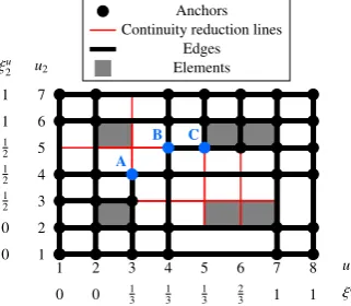
If a T-spline mesh is globally linearly dependent, the dependencies between anchors can be detected by transforming Equation (24) into a row echelon form by Gaussian elimination, Figure 5.
A T-spline mesh with globally linearly dependent blending functions cannot be used for analysis since in a finite element context, this results in a system of equations that cannot be solved.
4.1.2. Local linear independence
Repeating the procedure of the previous section at the elemental level, the condition for local linear independence is
rank(Ce) =ne fore= 1. . . E (27)
with the elemental B´ezier extraction operator Ce and the number of anchors ne with support in elemente. When Equation (27) holds, the size ofCeis
size(Ce) =ne×
d
Y
ℓ=1
pℓ+ 1
!
1 2 3 4 5 6 7 8 1
2 3 4 5 6 7
0 0 13 1 3
1 3
2
3 1 1
0 0 1 2 1 2 1 2 1 1
u1 u2
ξu 1
ξu 2
A
B C
Anchors Continuity reduction lines
Edges Elements
(a) Globally linearly dependent cubic T-spline mesh [8], transforming Equation (24) into row echelon form yields the following linear dependencies between the anchors A, B and C:−3NA
(ξ) + 3NB
(ξ) +NC
(ξ) = 0.
1 2 3 4 5 6 7 8 9 10
1 2 3 4 5 6 7 8 9
0 0 0 13
1 3
1 3
2
3 1 1 1
0 0 0 1 2 1 2 1 2 1 1 1
u1 u2
ξu 1
ξu 2
D
E F
Anchors Continuity reduction lines
Edges Elements
(b) Globally linearly dependent quartic T-spline mesh, transforming Equation (24) into row echelon form yields the following linear dependencies between the anchors D, E and F:−3ND
(ξ) + 2NE
(ξ) +NF
[image:10.595.102.263.73.213.2](ξ) = 0.
Figure 5. Globally linearly dependent T-spline meshes of cubic and of quartic polynomial degree.
4.1.3. Local linear independence with a square matrixCe
A subset of locally linearly independent T-spline meshes (i. e. when Equation (27) holds) can be defined when the following additional property is valid for each elemente
rank(Ce) =
d
Y
ℓ=1
pℓ+ 1 =ne fore= 1. . . E. (29)
When Equation (29) holds, the size ofCeis
size(Ce) =
d
Y
ℓ=1
pℓ+ 1
!
× d
Y
ℓ=1
pℓ+ 1
!
. (30)
Note, that Equation (29) implies Equation (27). Also, Equation (27) implies Equation (25) – local linear independence inherently results in global linear independence.
If a T-spline mesh is locally linearly dependent, then the non-zero coefficientsαeare obtained analogously to the global case by transforming
CT
eαe=0 (31)
into row echelon form. In Figure 6 examples are given for a locally linearly dependent T-spline mesh, a T-spline mesh for which Equation (27) holds and a T-spline mesh for which Equation (29) holds.
4.2. Partition of unity property for T-splines
1 2 3 4 5 1
2 3 4 5 6 7
0 0 12 1 1
0 0 1 4 2 4 3 4 1 1
u1 u2
ξu
1 ξu
2
b
G H
Anchors Continuity reduction lines
Edges Elements
(a) Locally linearly dependent T-spline mesh, ten anchors (blue) have a support in element b (dashed green); transforming Equation (31) into row echelon form yields the dependencies in element b between anchors G and H:6NG(ξ)−NH(ξ) = 0.
1 2 3 4 5
1 2 3 4 5 6 7
0 0 12 1 1
0 0 1 4 2 4 3 4 1 1
u1 u2
ξu
1 ξu
2
c
Anchors Continuity reduction lines
Edges Elements
(b) Locally linearly independent T-spline mesh;
rank(Ce) =ne for element c; in element c (dashed green) are only eight anchors (blue) with a support and thereforeCeis not a square matrix for element c.
1 2 3 4 5
1 2 3 4 5 6 7
0 0 12 1 1
0 0 1 3 2 3 2 3 1 1
u1 u2
ξu
1 ξu
2
Anchors Continuity reduction lines
Edges Elements
(c) Locally linearly independent T-spline mesh;
rank(Ce) = d
Q
ℓ=1
[image:11.595.103.259.72.212.2]pℓ+ 1fore= 1. . . E.
Figure 6. Local dependencies in a quadratic T-spline mesh.
4.2.1. Partition of unity property of the rational blending functionsRi
The multivariate rational T-spline blending function for an anchorican be constructed as
Ri(ξ) = w iNi(ξ)
n
P
j=1
wjNj(ξ)
(32)
with the weightwiassociated to anchori. Note that, in view of Equation (32), the rational blending functionsRialways form a partition of unity (allRisum to one).
4.2.2. Partition of unity property of the blending functionsNi
In [3] T-spline meshes have been classified according to the partition of unity property of the blending functionsNi,
n
X
i=1
βiNi(ξ) = 1, (33)
into
• Semi-standard T-spline meshes: someβi6= 1, • Non-standard T-spline meshes: no solution forβi.
We note, that only for standard T-spline meshes the blending functionsNiand the rational blending functionsRisatisfy the partition of unity property.
4.2.3. Partition of unity property of the blending functionsNiusing the B´ezier extraction operator We will now show how the global B´ezier extraction operator can be used to determine the partition of unity property of the blending functionsNi. Rewriting Equation (33) using Equation (18) yields
n
X
i=1
βiCiTB(ξ) = 1. (34)
Substituting Equations (13) and (17) into Equation (34) and elaboration gives
β1C1
1
T
+. . .+βnCn
1T
| {z }
γT
1
B1(ξ) +. . .+
β1C1
E T
+. . .+βnCn E
T
| {z }
γT E
BE(ξ) = 1. (35)
The Bernstein polynomialsBein Equation (35) form a partition of unity if and only ifγ
e=1for each elemente. This statement can be expressed in a vector-matrix format as
β1C1
1+. . .+βnCn1
.. .
β1C1
E+. . .+βnC n E
=
1
.. . 1
(36)
which is equivalent to
C1 . . . Cn
β1
.. .
βn
=1. (37)
With the global B´ezier extraction operatorCin Equation (14) we obtain
CTβ=1. (38)
The row echelon form of Equation (38) then provides the means to assess whether a T-spline mesh is standard, semi-standard or non-standard.
1 2 3 4 5 1 2 3 4 5 6 7
0 0 12 1 1
0 0 1 3 1 3 2 3 1 1 u1 u2 ξu 1 ξu 2 Anchors Continuity reduction lines
Edges Elements
(a) Standard,rank(Ce) = d
Q
ℓ=1
pℓ+ 1fore= 1. . . E.
1 2 3 4 5
1 2 3 4 5 6 7
0 0 12 1 1
0 0 1 4 2 4 3 4 1 1 u1 u2 ξu 1 ξu 2 Anchors Continuity reduction lines
Edges Elements
(b) Non-standard,rank(C) =n.
1 2 3 4 5
1 2 3 4 5 6 7
0 0 12 1 1
0 0 1 3 2 3 2 3 1 1 u1 u2 ξu 1 ξu 2 Anchors Continuity reduction lines
Edges Elements
(c) Standard,rank(Ce) = d
Q
ℓ=1
pℓ+ 1fore= 1. . . E.
1 2 3 4 5
1 2 3 4 5 6 7
0 0 12 1 1
0 0 1 4 2 4 3 4 1 1 u1 u2 ξu 1 ξu 2 Anchors Continuity reduction lines
Edges Elements
(d) Non-standard,rank(Ce) =nefore= 1. . . E.
1 2 3 4 5
1 2 3 4 5 6 7
0 0 12 1 1
0 0 1 3 2 3 2 3 1 1 u1 u2 ξu 1 ξu 2 Anchors Continuity reduction lines
Edges Elements
(e) Standard,rank(Ce) = d
Q
ℓ=1
pℓ+ 1fore= 1. . . E.
1 2 3 4 5
1 2 3 4 5 6 7
0 0 12 1 1
0 0 1 4 2 4 3 4 1 1 u1 u2 ξu 1 ξu 2 Anchors Continuity reduction lines
Edges Elements
[image:13.595.94.495.69.594.2](f) Semi-standard,rank(C) =n.
Figure 7. Classification of quadratic T-spline meshes according to the level of linear independence and the partition of unity property. (a), (c) and (e) are standard T-spline meshes, changing the knot intervals results
1 2 3 4 5 1 2 3 4 5 6 7
0 0 12 1 1
0 0 1 3 1 3 2 3 1 1 u1 u2 ξu 1 ξu 2 Anchors Continuity reduction lines
Edges Elements
(a) Standard,rank(Ce) = d
Q
ℓ=1
pℓ+ 1fore= 1. . . E.
1 2 3 4 5
1 2 3 4 5 6 7
0 0 12 1 1
0 0 1 4 2 4 3 4 1 1 u1 u2 ξu 1 ξu 2 Anchors Continuity reduction lines
Edges Elements
(b) Non-standard,rank(C) =n.
1 2 3 4 5
1 2 3 4 5 6 7
0 0 12 1 1
0 0 1 3 2 3 2 3 1 1 u1 u2 ξu 1 ξu 2 Anchors Continuity reduction lines
Edges Elements
(c) Standard,rank(Ce) = d
Q
ℓ=1
pℓ+ 1fore= 1. . . E.
1 2 3 4 5
1 2 3 4 5 6 7
0 0 12 1 1
0 0 1 4 2 4 3 4 1 1 u1 u2 ξu 1 ξu 2 Anchors Continuity reduction lines
Edges Elements
(d) Non-standard,rank(Ce) =nefore= 1. . . E.
1 2 3 4 5
1 2 3 4 5 6 7
0 0 12 1 1
0 0 1 3 2 3 2 3 1 1 u1 u2 ξu 1 ξu 2 Anchors Continuity reduction lines
Edges Elements
(e) Standard,rank(Ce) = d
Q
ℓ=1
pℓ+ 1fore= 1. . . E.
1 2 3 4 5
1 2 3 4 5 6 7
0 0 12 1 1
0 0 1 4 2 4 3 4 1 1 u1 u2 ξu 1 ξu 2 Anchors Continuity reduction lines
Edges Elements
[image:14.595.94.494.69.594.2](f) Semi-standard,rank(C) =n.
Figure 8. Classification of cubic T-spline meshes according to the level of linear independence and the partition of unity property. (a), (c) and (e) are standard T-spline meshes, changing the knot intervals results
4.2.4. Affine transformation requires partition of unity
Any T-spline surface T in the physical domain (xℓ) can be expressed by the mapping from the sub-parameter (ξℓ) domain as follows
T(ξ) =
n
X
i=1
Ri(ξ)Pi (39)
whereRiare the rational blending functions andPi= (xi
1, xi2)are the control points associated to
anchori. Applying a transformation to the control pointsP of the form
PT=AP+b, (40)
with the control pointsPTafter transformation, results in an affine transformation since the rational
blending functionsRiin Equation (39) form a partition of unity.
However, when the T-spline in Equation (39) would have been defined with the blending functions
Niinstead of the rational blending functionsRi, then an affine transformation is only obtained for standard T-spline meshes since semi-standard and non-standard T-spline meshes do not have the partition of unity property for the blending functionsNi, see also Figure 9 with a rigid body motion applied to the control points of the anchors.
Initial physical mesh
Transformed physical mesh Anchors
Element boundaries
(a) Rational blending functionsRi.
Initial physical mesh
Transformed physical mesh Anchors
Element boundaries
(b) Blending functionsNi.
Figure 9. Applying a rigid body motion to the control points of the anchors results in an affine transformation when the partition of unity property is fulfilled. (a) An affine transformation for the semi-standard T-spline mesh in Figure 8(f) is obtained for the rational blending functionsRi; (b) using the blending functionsNi
instead ofRiin Equation (39) gives no affine transformation – the element boundaries are different – since theNido not form a partition of unity for semi-standard meshes.
The patch test is always satisfied when an affine transformation is possible, i. e. for the rational blending functionsRi, and for the blending functionsNiof a standard T-spline mesh.
4.3. Standard T-splines are locally linearly independent with a square matrixCe
We will show next that standard T-spline meshes are always locally linearly independent and that the elemental B´ezier operatorsCeare always a square matrix. We start with the global partition of unity property of standard T-spline meshes,
n
X
i=1
βiNi(ξ) = 1 withβi= 1. (41)
The global partition of unity property for standard T-spline meshes in Equation (41) implies the local partition of unity property for each elemente
ne
X
i=1
Now we add to Equation (42) the expression
ne
X
i=1
αi
eNi(ξ) = 0 (43)
which results in
ne
X
i=1
(βei+αie)Ni(ξ) = 1 withβei = 1. (44)
If there existed an anchoriwithαi
e6= 0in Equation (44), the T-spline mesh would not be a standard T-spline mesh (see also the proof in [16] for the global case). Therefore, the only solution isαi
e= 0 fori= 1. . . nein Equation (44) which means that we have for each elementein Equation (43)
ne
X
i=1
αi
eNi(ξ) = 0 withαie= 0. (45)
Hence, the global partition of unity property implies local linear independence of the T-spline mesh. However, we do not know yet whetherCeis a square matrix or not. To further pursue this issue, we write the resultβi
e= 1in Equation (42) as follows
1 0 · · · 0 0 1 . . . 0
..
. ... . .. ...
0 0 . . . 1
β1
e .. .
βne e
=Ieβe=1 (46)
whereIeis the unity matrix
Ie= diag(1,1, . . . ,1). (47)
It is important to note that the size of the unity matrixIeis
size(Ie) =
d
Y
ℓ=1
pℓ+ 1
!
× d
Y
ℓ=1
pℓ+ 1
!
(48)
and therefore,ne= d
Q
ℓ=1
pℓ+ 1. By writing Equation (38) for elementein an elemental form
CTeβe=1, (49)
we can draw the conclusion that Equation (46) is the row echelon form of Equation (49). Hence, we can infer thatCehas the same size asIeand thatCeis also a square matrix,
size(Ce) = size(I) =
d
Y
ℓ=1
pℓ+ 1
!
× d
Y
ℓ=1
pℓ+ 1
!
. (50)
We recall that the global partition of unity property results in locally linearly independent blending functions. With Equation (50) this leads to the conclusion that we have the case in Equation (29) sinceCeis a square matrix. In sum, all standard T-splines have the following property
rank(Ce) =
d
Y
ℓ=1
pℓ+ 1 =ne fore= 1. . . E. (51)
4.4. Analysis-suitable T-splines
Analysis-suitable T-splines have been defined in [9]. In order to detect them, the extended T-spline mesh was introduced, and a mesh was deemed analysis-suitable when there are no two orthogonal T-node extensions which intersect in the extended T-spline mesh. This definition holds for any knot interval and is of topological nature; it allows to distinguish between analysis-suitable and non-analysis-suitable T-splines.
The new approach in this paper which is based on the B´ezier extraction operator is an algebraic viewpoint and allows a classification of T-splines into standard, semi-standard and non-standard with Equation (38).
Figure 10 reveals that a standard T-spline is not necessarily an analysis-suitable T-spline. In Figure 10, T-node extensions intersect in the extended T-spline mesh and the T-spline meshes are therefore non-analysis-suitable. From Figure 8(a), 8(c) and 8(e) we know that these T-spline meshes are standard.
1 2 3 4 5
1 2 3 4 5 6 7
0 0 12 1 1
0 0
1 3 1 3 2 3
1 1
u1 u2
ξu 1 ξu
2
Anchors Continuity reduction lines
Edges Elements T-node extensions
(a) T-node extensions for the T-spline mesh in Figure 8(a).
1 2 3 4 5
1 2 3 4 5 6 7
0 0 12 1 1
0 0
1 3 2 3 2 3
1 1
u1 u2
ξu 1 ξu
2
Anchors Continuity reduction lines
Edges Elements T-node extensions
(b) T-node extensions for the T-spline mesh in Figure 8(c).
1 2 3 4 5
1 2 3 4 5 6 7
0 0 12 1 1
0 0
1 3 2 3 2 3
1 1
u1 u2
ξu 1 ξu
2
Anchors Continuity reduction lines
Edges Elements T-node extensions
[image:17.595.99.501.272.628.2](c) T-node extensions for the T-spline mesh in Figure 8(e).
5. LOCAL REFINEMENT OF STANDARD, SEMI-STANDARD AND NON-STANDARD T-SPLINES BY ADDING ANCHORS
In this section we show how standard, semi-standard and non-standard T-spline meshes of even and odd polynomial degree can be refined locally by adding anchors using information from the B´ezier extraction operator.
A requirement for the refinement algorithm is that the initial and the refined T-spline mesh are nested – this condition will be defined in the following section, together with a method to fulfil it using the B´ezier extraction operator. We also show how the location of the control points in the refined T-spline mesh can be obtained. Afterwards, we explain the algorithm for the local refinement of T-splines and give some examples. In the examples we first focus on refining standard T-spline meshes (Section 5.4, Appendix A) followed by an example to show that also non-standard meshes can be refined locally by adding anchors (Appendix B).
5.1. Computation of the refinement matrix and nesting behaviour
A refinement matrixMof sizen×nRgives the relation between the blending functionsNRof a refined mesh withnRanchors and the blending functionsN of an initial mesh which hasnanchors
N(ξ) =MNR(ξ). (52)
Expressing the blending functions on both sides using the Bernstein polynomials, Equation (16), gives
CBR(ξ) =M CRBR(ξ), (53)
while the blending functions N on the initial mesh must be defined in terms of the elements of the refined mesh with the Bernstein polynomials BR. The linear independence of the Bernstein polynomialsBRin Equation (53) results in
C=M CR. (54)
The coefficients of a row of the refinement matrix M can be evaluated as follows. Expanding Equation (54) using Equation (14) yields
C1T .. . CnT
=
M1T .. . MnT
C1RT .. . CnRR T
. (55)
Applying the transpose to both sides results in
C1 . . . Cn=C1R . . . CnRR M1 . . . Mn (56)
which makes it possible to determine the rowsMiT fori= 1. . . nof the refinement matrixMby transforming the systems
Ci=CRTMi fori= 1. . . n (57)
into a row echelon form. In the case that there is no solution for theMifor anchoriin Equation (57), the initial and the refined T-spline mesh are not nested, which means that it is not possible to represent all blending functions N of the initial T-spline mesh as a linear combination of the blending functions NR of the refined T-spline mesh. One can resolve this as will be explained in Section 5.4 (quadratic case,pℓ= 2) and Appendix A (cubic case,pℓ= 3).
β=1) and using the rowsMiT of the refinement matrixMfrom Equation (57) results in
1 =
n
X
i=1
βiNi(ξ) = n
X
i=1
βiMiT
NR(ξ) =
nR
X
j=1
βRjNRj(ξ) (58)
where the coefficientsβRare given by
βR=MTβ. (59)
From Equation (59) it can be concluded that there always exists a solution for the coefficientsβR when nestedness is ensured (Mexists) and therefore the refined T-spline mesh can only be a standard or semi-standard T-spline mesh when the initial mesh is standard.
5.2. Determination of the coordinates for the anchors in the refined T-spline mesh
In this section we assume that the initial and the refined T-spline mesh are nested. We show how the coordinates and weights of the anchors in a refined T-spline mesh can be determined. The weighted (polynomial) curve of Equation (39) is given by [20]
Tw(ξ) = n
X
i=1
Ni(ξ)Piw (60)
with the weighted control points
Piw= (wixi1, wixi2, wi). (61)
We require that the refined and the initial weighted curves –Tw RandTw, respectively – represent the same geometry
Tw R(ξ) =Tw(ξ), (62)
and insert Equation (60) into the left- and right-hand side of Equation (62) to obtain nR
X
j=1
NRj(ξ)Pjw R=
n
X
i=1
Ni(ξ)Piw. (63)
Using the B´ezier extraction operator subsequently gives nR
X
j=1
CjRTBR(ξ)Pjw R= n
X
i=1
CiTBR(ξ)Piw (64)
or, since the Bernstein polynomialsBRare linearly independent
nR
X
j=1
CjRTPjwR=
n
X
i=1
CiTPiw. (65)
Elaborating Equation (65) yields
C1R . . . CnR R
P1w R .. . PnR
w R
=
C1 . . . Cn
P1w .. . Pnw
(66)
or, in the global form
C R
T
Pw R=CTP
w, (67)
so that with Equation (54), we obtain
C R
TP
wR=CRTMTPw. (68)
Hence, the weighted control pointsPw Rfor the refined mesh follow from
5.3. The algorithm for local refinement of standard T-splines
In our local refinement algorithm (see also Algorithm 1) for standard T-splines we proceed as follows: after inserting new anchors into the T-spline mesh (refining), we check whether the necessary condition for standard T-spline meshes, Equation (51), holds. If this is not the case, the mesh resulting from local refinement will not be standard either. Then, Equation (31) plays a key role: it allows us to determine whetherCeis a square matrix or not, but also, when presented in row echelon form, to detect and remove linear dependencies, leading to the necessary condition for standard T-spline meshes in Equation (51). Once Equation (51) is fulfilled, we evaluate each row of the refinement matrixMin Equation (57). Should the blending functions of some anchors of the initial mesh not be nested in the refined mesh, then we modify the mesh accordingly. Finally, when nestedness is satisfied, Equation (38) is assessed whetherβ=1holds. If not, then we have a semi-standard mesh according to Equation (59) and anchors are added to the mesh within the support of anchors for whichβi 6= 1. Otherwise, the initial and the refined mesh are nested standard T-spline meshes.
// Start with a standard T-spline mesh // Number of refinement steps:N fori= 1 :Ndo
RefinementSuccessful = 0; whileRefinementSuccessful = 0do
// Check whether necessary condition for standard T-splines in Equation (51) holds:
ifCe6= d
Q
ℓ=1
(pℓ+ 1) fore= 1. . . E then
// add additional anchors by inspecting the B´ezier extraction operator in Equation (31): // (a) ensure thatCeis a square matrix
// (b) remove linear dependencies else
// Check with Equation (57) whether the initial and the refined mesh are nested: if Refinement matrixMcannot be computed then
// add additional anchors by assessing the B´ezier extraction operators of the initial and the refined mesh: localise, which anchors are not nested in Equation (57)
else
// Check whether T-spline mesh is standard by assessing Equation (38): ifβ6=1then
// mesh is semi-standard according to Equation (59)
// add anchors to the mesh within the support of the anchorsifor whichβi6
= 1
else
// Compute the weighted control pointsPw Rof the refined mesh using Equation (69)
RefinementSuccessful = 1; end
end end end end
Algorithm 1: Local refinement algorithm based on the insertion of new anchors for standard T-spline meshes.
5.4. Local refinement of standard T-splines of even degree by adding anchors
This section explains how the necessary condition for standard T-spline meshes in Equation (51) and nestedness for meshes of even degree can be enforced using the B´ezier extraction operator. It should be noted, that in order to be able implement the methods described in the following, the local knot vectors for each anchor are required in the index (uℓ) and sub-parameter (ξℓ) domain – it is not sufficient to have only access to the B´ezier extraction operator.
Initial refinement
[image:21.595.103.468.129.288.2]We consider the quadratic standard T-spline mesh in the index domain and the physical domain in Figure 11. It is refined by insertion of an anchor which results in the rectangle[ξ2
1, ξ14]×[ξ23, ξ25]
being split vertically, see Figure 12(a).
1 2 3 4 5
1 2 3 4 5 6 7
0 0 1
2 1 1
0 0 1 3 1 3 2 3 1 1
u1 u2
ξu
1 ξu
2
Anchors Continuity reduction lines
Edges Elements
(a)
Anchors Element corners Element boundaries
(b)
Figure 11. Initial quadratic standard T-spline mesh in (a) the index domain and (b) the physical domain.
1 2 3 4 5
1 2 3 4 5 6 7
0 0 12 1 1
0 0 1 3 1 3 2 3 1 1
u1 u2
ξu
1 ξu
2
Anchors Continuity reduction lines
Edges Elements
(a)
1 2 3 4 5
1 2 3 4 5 6 7
0 0 12 1 1
0 0 1 3 1 3 2 3 1 1
u1 u2
ξu
1 ξu
2
b Anchors Continuity reduction lines
Edges Elements
(b)
Figure 12. (a) Refined quadratic non-standard T-spline mesh from Figure 11(a) in the index domain. (b) The T-spline mesh is locally linearly independent – but as only eight anchors (blue) have a support in element b
(dashed green line),Ceis not a square matrix for element b.
Ensuring thatCeis a square matrix
The resulting mesh is locally linearly independent, but non-standard and,Ceis not a square matrix for all elements. Indeed, for element b (bounded by a dashed green line), we haverank(Ce) =ne, as there are only eight anchors (blue) with a support,ne= 8, see Figure 12(b). Hence, additional anchors need to be inserted in order to obtain a square matrix Ce. Each local knot vector of the blue anchors with support in element b in Figure 12(b) contains the sub-parameter values of the boundaries of element b –[0,12]×[13,23]in theξ1direction and theξ2direction, respectively, except
for the anchors A and B in Figure 13(a). The local knot vectors of the anchors A and B in theξ1
direction do not contain the sub-parameter valueξ1=12. Therefore, rectangle c needs to be split.
1 2 3 4 5 1
2 3 4 5 6 7
0 0 12 1 1
0 0 1 3 1 3 2 3 1 1
u1 u2
ξu
1 ξu
2
b
A B
c Anchors Continuity reduction lines
Edges Elements
(a)
1 2 3 4 5
1 2 3 4 5 6 7
0 0 12 1 1
0 0 1 3 1 3 2 3 1 1
u1 u2
ξu
1 ξu
2
Anchors Continuity reduction lines
Edges Elements
[image:22.595.103.481.70.229.2](b)
Figure 13. Procedure to obtain a square matrixCe. (a) The local knot vectors of the anchors A and B (blue)
do not contain the sub-parameter valueξ1= 12, which is a boundary of element b (dashed green). The local
knot vectors of all other anchors with support in element b (see Figure 12(b)) contain the sub-parameter values0,12in theξ1direction and 13,23in theξ2direction –[0,12]×[13,23]represents the boundary values of
element b in the sub-parameter domain. Hence, the rectangle c needs to be split so that the local knot vectors of the anchors A and B also contain the knotξ1= 12. (b) The resulting standard mesh and the initial mesh
in 11(a) are not nested.
Nestedness
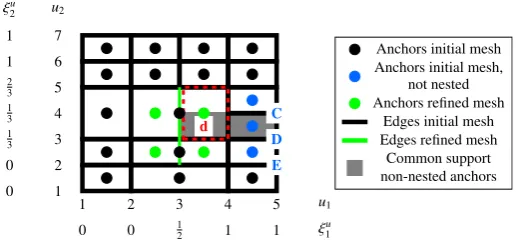
The initial T-spline mesh in Figure 11(a) and the refined mesh in Figure 13(b) are not nested: the blending functions of anchors C, D and E (see mesh in Figure 14) cannot be expressed as a linear combination of the blending functions of the refined mesh in Figure 13(b). This can be identified by inspection of the row echelon form of Equation (57) for these anchors.
1 2 3 4 5
1 2 3 4 5 6 7
0 0 12 1 1
0 0
1 3 1 3 2 3
1 1
u1
u2
ξu
1 ξu
2
d
E D C
Anchors initial mesh Anchors initial mesh,
not nested Anchors refined mesh
Edges initial mesh Edges refined mesh Common support non-nested anchors
Figure 14. Superposition of the initial T-spline mesh in the index domain from Figure 11(a) and the refined mesh in Figure 13(b). Transforming Equation (57) into row echelon form gives no results for the anchors C, D and E (blue) since the meshes in Figure 11(a) and Figure 13(b) are not nested. Edges and anchors from the refined mesh in Figure 13(b), which were added during refinement, are inserted in the initial mesh from Figure 11(a) and marked with green. Within the grey domain all three anchors C, D and E from the initial mesh have a support, while the grey domain is bounded by the newly inserted green edges. In this grey domain an additional anchor needs to be inserted, i. e. the dashed red rectangle d needs to be subdivided, see
Figure 15.
[image:22.595.172.432.428.549.2]refined mesh has now the sought properties: it is standard and is nested with the initial (non-refined) mesh, i. e. the blending functionN of each anchor in Figure 11(a) can be represented as a linear combination of the blending functionsNRof the anchors in the refined mesh in Figure 15(a).
Refined physical mesh
So far, refinement has only been considered in the index domain in order to obtain a standard and nested T-spline mesh. Next, the evaluation of the weighted control points in the physical domain is addressed.
The location of the weighted control points for the refined mesh Pw R is determined using Equation (69). The physical mesh is shown in Figure 15(b) which preserves the same geometry as the physical mesh in Figure 11(b). This can be observed by comparing for instance the shape of the element boundaries of the initial and the refined physical mesh.
1 2 3 4 5
1 2 3 4 5 6 7
0 0 1
2 1 1
0 0 1 3 1 3 2 3 1 1
u1 u2
ξu
1 ξu
2
Anchors Continuity reduction lines
Edges Elements
(a)
Anchors Element corners Element boundaries
[image:23.595.102.471.227.387.2](b)
Figure 15. Refined quadratic T-spline mesh of Figure 11 in (a) the index domain and (b) the physical domain. This T-spline mesh is standard and nested with the initial T-spline mesh of Figure 11.
5.4.2. Example 2: Removing linear dependencies
Initial refinement
As a next example, the initial quadratic T-spline mesh in Figure 11 is now refined as shown in Figure 16(a).
Removing linear dependencies
The T-spline mesh of Figure 16(a) is non-standard using Equation (38). Furthermore, the necessary condition Equation (51) is not fulfilled. Transforming Equation (31) into row echelon form yields the dependencyNF(ξ)−NG(ξ) = 0in element f. In order to break this dependence, new anchors need to be inserted. In the following, it will be shown how to identify potential locations for these new anchors and how to select the ideal one.
1 2 3 4 5 1 2 3 4 5 6 7
0 0 12 1 1
0 0 1 3 1 3 2 3 1 1 u1 u2 ξu 1 ξu 2 f F G Anchors Continuity reduction lines
Edges Elements
(a) The T-spline mesh is locally linearly dependent – the row echelon version of Equation (31) gives the dependencyNF
(ξ)−NG
(ξ) = 0in element f.
1 2 3 4 5
1 2 3 4 5 6 7
0 0 12 1 1
0 0 1 3 1 3 2 3 1 1 u1 u2 ξu 1 ξu 2 F G g h Anchors Edges
[image:24.595.103.259.67.207.2] [image:24.595.318.476.82.207.2](b) Extension lines (solid blue) for the anchors F and G intersect at the location of the green squares. The rectangles g and h (dashed red line) contain the green squares. Rectangle g cannot be further subdivided. All options for subdividing rectangle h are given in Figure 17.
Figure 16. Refined (non-standard) quadratic T-spline mesh from Figure 11(a) in the index domain.
1 2 3 4 5
1 2 3 4 5 6 7
0 0 1
2 1 1
0 0 1 3 1 3 2 3 1 1 u1 u2 ξu 1 ξu 2 Anchors Edges
(a) Standard, not nested.
1 2 3 4 5
1 2 3 4 5 6 7
0 0 1
2 1 1
0 0 1 3 1 3 2 3 1 1 u1 u2 ξu 1 ξu 2 Anchors Edges
(b) Standard, nested.
1 2 3 4 5
1 2 3 4 5 6 7
0 0 1
2 1 1
0 0 1 3 1 3 2 3 1 1 u1 u2 ξu 1 ξu 2 Anchors Edges
(c) Standard, not nested.
1 2 3 4 5
1 2 3 4 5 6 7
0 0 1
2 1 1
0 0 1 3 1 3 2 3 1 1 u1 u2 ξu 1 ξu 2 Anchors Edges
(d) Standard, nested.
1 2 3 4 5
1 2 3 4 5 6 7
0 0 1
2 1 1
0 0 1 3 1 3 2 3 1 1 u1 u2 ξu 1 ξu 2 Anchors Edges (e) Non-standard.
1 2 3 4 5
1 2 3 4 5 6 7
0 0 1
2 1 1
0 0 1 3 1 3 2 3 1 1 u1 u2 ξu 1 ξu 2 Anchors Edges (f) Non-standard.
1 2 3 4 5
1 2 3 4 5 6 7
0 0 1
2 1 1
0 0 1 3 1 3 2 3 1 1 u1 u2 ξu 1 ξu 2 Anchors Edges (g) Non-standard.
Figure 17. All possible subdivisions for the rectangle h in Figure 16(b): the dashed orange lines indicate the new edges to be inserted, the orange points denote the location of the new anchors.
[image:24.595.103.488.321.633.2]anchors for the options in Figure 17. This information can be used in order to determine the best location and optimum number of additional anchors.
Table I. Summary of the number of pairs of anchors with linearly dependent blending functions, number of non-square matricesCe, nestedness and number of additionally inserted anchors for the options in Figure 17.
Figure 17(a) 17(b) 17(c) 17(d) 17(e) 17(f) 17(g)
Number of pairs of anchors
0 0 0 0 0 0 0
with linearly dependent blending functions Number of non-square
0 0 0 0 1 2 2
matricesCe
Nestedness ✗ ✓ ✗ ✓ ✗ ✗ ✗
Number of additional anchors 2 3 3 4 2 3 3
According to Figure 17 and Table I, only the options (b) and (d) are suitable for refinement of the T-spline mesh in Figure 11 since they are standard and nested with the initial mesh. From an implementational point of view, one could select the option which introduces the smallest amount of new anchors, i. e. option (b).
In case that no refinement option results in a standard and nested T-spline mesh, one can select either the option with the smallest number of pairs of anchors with linearly dependent blending functions or the option with the smallest number of non-square matricesCeand then continue with the next refinement step until a standard and nested mesh is obtained, see Appendix C.
5.5. Summary for the local refinement of standard T-splines
The examples for the local refinement of standard T-spline meshes by adding anchors demonstrate that the B´ezier extraction operator allows to:
• enforce the necessary condition in Equation (51) for standard T-spline meshes:
– when the T-spline mesh is locally linearly independent but we do not have a square matrixCefor each elemente, the B´ezier extraction operator shows, which element does not have enough anchors with a support (Figure 13(a));
– when there are local linear dependencies, the B´ezier extraction operator shows, where new anchors and edges need to be inserted (Figure 16(b))
• pinpoint for which blending functions two T-spline meshes are not nested (Figure 14).
We have found that when the necessary condition in Equation (51) is fulfilled and the refinement matrix Min Equation (57) can be computed, we always obtain a nested standard T-spline mesh. We have not experienced a single case where this resulted in a nested semi-standard T-spline mesh. However, should such a case arise, one can pinpoint for which anchorsβi
R6= 1using Equation (59) and insert an additional anchor in the supported domain of these anchors.
The local refinement of standard T-spline meshes of odd degree is treated in Appendix A. Furthermore, Appendix B demonstrates that also non-standard T-splines can be refined locally when nestedness exists.
6. HIERARCHICAL REFINEMENT OF STANDARD, SEMI-STANDARD AND NON-STANDARD T-SPLINES USING THE RECONSTRUCTION OPERATOR
analysis-suitable T-splines. Here, we show how the idea of this concept can also be applied to standard, semi-standard and non-standard T-spline meshes.
6.1. Splitting elements
The hierarchical refinement algorithm based on the reconstruction operator requires local linear independence. Moreover, it requires thatCeis a square matrix for the elementethat is subdivided,
rank(Ce) =
d
Y
ℓ=1
pℓ+ 1 (70)
since the reconstruction operator, defined as
Re=C−1
e , (71)
is needed. Therefore, for this hierarchical refinement algorithm the B´ezier extraction operator plays again a key role: when Equation (70) is satisfied for elemente, this element can be refined hierarchically. Thus, this algorithm can be applied to standard, semi-standard and non-standard T-spline meshes.
Consider an element with range[−1,1]and suppose that we want to split it in half:[−1,0]and
[0,1]. The first Bernstein basisB1
1with the knot vector{−1,−1,−1,1}(black curve) in Figure 18 in
the element[−1,1]can be defined in the two sub-elements[−1,0]and[0,1]as a linear combination of the Bernstein polynomials in the two sub-elements: the Bernstein basis functions for the left part of the element with support in[−1,0]are given by the local knot vectors
B11lfor{−1,−1,−1,0}, B21lfor{−1,−1,0,0}, B13lfor{−1,0,0,0}. (72)
−1 −0.8 −0.6 −0.4 −0.2 0 0.2 0.4 0.6 0.8 1
0 0.2 0.4 0.6 0.8 1
ξ1
B1
[image:26.595.208.387.392.536.2]1l(ξ1) B21l(ξ1) B31l(ξ1) B11(ξ1)
Figure 18. The Bernstein polynomial B11 with support over the element[−1,1]can be expressed in the sub-element el with range[−1,0]as a linear combination of the Bernstein polynomials B1al:B11(ξ1) =
B11l(ξ1) +12B21l(ξ1) +14B31l(ξ1).
The Bernstein polynomial B1
1 in the left part of the element (solid black line) can now be
expressed as a linear combination of the Bernstein polynomialsBi
1las follows
B11(ξ1) =
1 1
2 1 4
B1
1l(ξ1)
B2 1l(ξ1)
B3 1l(ξ1)
. (73)
The coefficients in Equation (73) can either be obtained using the algorithm in [7] for the knot vector {−1,−1,−1,1}with an interior knot (causing a discontinuity) atξ1= 0or, alternatively, using the
the range[0,1]) gives
B1
1(ξ1)
B2 1(ξ1)
B3 1(ξ1)
| {z } B1(ξ1)
=
1 1
2 1 4
0 1
2 1 2
0 0 1
4
| {z }
A1l
B1
1l(ξ1)
B2 1l(ξ1)
B3 1l(ξ1)
| {z }
B1l(ξ1)
+
1 4 0 0 1 2
1 2 0 1 4
1 2 1
| {z }
A1r
B1
1r(ξ1)
B2 1r(ξ1)
B3 1r(ξ1)
| {z }
B1r(ξ1)
. (74)
Hence, the Bernstein polynomialsB1 over one elementewith the span[−1,1]can be expressed as a linear combination of the Bernstein polynomialsB1landB1rover the two smaller elements
elwith the span[−1,0]anderwith the span[0,1]. Extending Equation (74) into more dimensions gives
B(ξ) =AlB
l(ξ) +ArBr(ξ). (75)
We next assume that the B´ezier extraction operator is known for the original, single elementCe and for the two sub-elementsCe landCe r. Then, we can express the weighted curveT
w ewith the weighted control pointsPiw eover elementeusing Equation (75)
Twe(ξ) =
ne
X
i=1
CieTB(ξ)Piw e =
ne
X
i=1
CieT AlBl(ξ) +ArBr(ξ)Pi
we (76)
and over the two sub-elements
Tw e(ξ) =Twe l(ξ) +Tw e r(ξ) =
ne l
X
j=1
Cje lTBl(ξ)Pjw e l+ ne r
X
k=1
Cke rTBr(ξ)Pkw e r (77)
with the weighted control pointsPw e l andPwe rfor elementelander, respectively. Comparing Equation (76) and Equation (77) results in
ne
X
i=1
Cie T
AlBl(ξ)Piw e= ne l
X
j=1
Cje lTBl(ξ)Pjwe l (78)
ne
X
i=1
Cie T
ArBr(ξ)Piw e= ne r
X
k=1
Cke r T
Br(ξ)Pkw e r (79)
or in vector-matrix form
CeTAlP
we =Ce l T
Pwe l, (80)
CeTArPwe =Ce rTPwe r. (81)
Hence, the weighted coordinates of the two sub-elements are obtained with the reconstruction operator in Equation (71) as
Pwe l =Re lTCeTAlPwe, Pwe r=Re rTCeTArPwe. (82)
6.2. Example
As an example we consider the quadratic non-standard T-spline mesh of Figure 19 which is globally linearly independent but locally linearly dependent.
The dashed green element b is now divided vertically into two sub-element bland brwith range
[0,1
4]×[ 2 4,
3 4]and [
1 4,
1 2]×[
2 4,
3
4], i. e. the knot valueξ1= 1
4 is inserted in element b. Element b
1 2 3 4 5 1
2 3 4 5 6 7
0 0 12 1 1
0 0 1 4 2 4 3 4 1 1
u1 u2
ξu
1 ξu
2
A b
Anchors Continuity reduction lines
Edges Elements
Figure 19. Non-standard, globally linearly independent T-spline mesh in the index domain (from Figure 7(b)). Element b (dashed green line) with range[0,12]×[24,34]is split vertically into two sub-elements bl and brwith range[0,41]×[24,34]and[14,12]×[24,34], respectively. Each local knot vector associated to
a blue anchor (i. e. those having a support in element b) needs to be modified. For instance, the anchor A with ΞA1 ={0,0,0,1}becomesΞA1l={0,0,0,14}in element blandΞA1r={0,0,14,1}in element br.
ΞA1 ={0,0,0,1}remains unchanged for the other elements. The modified local knot vectors for the other
blue anchors are given in Appendix D.
which are obtained as follows. We pick from each blue anchoriwhich has a support over element b in Figure 19 the local knot vectorΞi
1. Then we insert into this local knot vector the knot value
ξ1=14 and split the resulting knot vector into two knot vectors of lengthpℓ+ 2, where one knot vector contains the firstpℓ+ 2entries and the other one the lastpℓ+ 2entries. For instance, taking the anchor A in Figure 19 gives the local knot vectorΞA
1 ={0,0,0,1}. The local knot vectors for
the elements bl and br are thenΞA1l={0,0,0,41} and ΞA1r={0,0,14,1}. We note that the local
knot vectorΞA
1 is modified only in the elements bland br, while for the other elementsΞA1 remains
unchanged. The local knot vectors for the blue anchors in the sub-elements bland br are given in Appendix D.
The initial non-standard T-spline mesh and the hierarchically refined non-standard T-spline mesh in the physical domain are depicted in Figure 20. Both physical meshes represent the same geometry.
Anchors Element corners Element boundaries
(a)
Initial anchors
Hierarchical anchors for bl
Hierarchical anchors for br
Element corners
Element boundaries
(b)
[image:28.595.212.366.66.208.2] [image:28.595.124.467.485.659.2]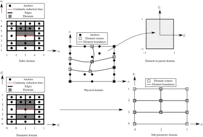


![Figure 10. Extended T-spline meshes for Figure 8(a), 8(c) and 8(e); these standard T-spline meshes arenon-analysis-suitable according to [9] since T-node extensions intersect in the extended T-spline mesh.](https://thumb-us.123doks.com/thumbv2/123dok_us/7895173.186986/17.595.99.501.272.628/extended-standard-analysis-suitable-according-extensions-intersect-extended.webp)